
Establishing Two-Dimensional Dependencies for Multi-Label Image Classification


Abstract
1. Introduction
- A.
- Establishing effective long-range spatial feature dependencies.
- B.
- Establishing global label semantic dependencies.
- We propose a Two-Dimensional Dependency Model (TDDM) for MLIC, which can simultaneously establish effective long-range spatial feature dependencies and global label semantic dependencies. This approach addresses the challenges of capturing the feature dependencies between distant targets in image feature extraction and incomplete understanding of the semantic dependencies between labels. To the best of our knowledge, this is the first multi-label image classification network that considers both problems simultaneously.
- We propose a Feature Fusion Module (FFM) and a Feature Enhancement Module (FEM), which effectively integrate image feature information from different spatial positions while enhancing and enriching high-dimensional abstract information. In terms of semantic extraction, we design a Global Relationship Extraction Module (GREM) to enhance the fusion of global relationships.
- We conducted experiments comparing our method with state-of-the-art methods on commonly used benchmark datasets. The results show that our method has superior computational performance. Specifically, our model achieves mAPs of 96.5% on PASCAL VOC 2007, 96.0% on PASCAL VOC 2012, and 85.2% on MS-COCO. The datasets and source code can be accessed from https://github.com/12pid/TDDM, accessed on 2 March 2025.
2. Related Work
2.1. Traditional Multi-Label Classification Methods
2.2. Deep Learning Methods for MLIC
2.3. Graph Structure Methods for MLIC
3. Method
3.1. Preliminaries
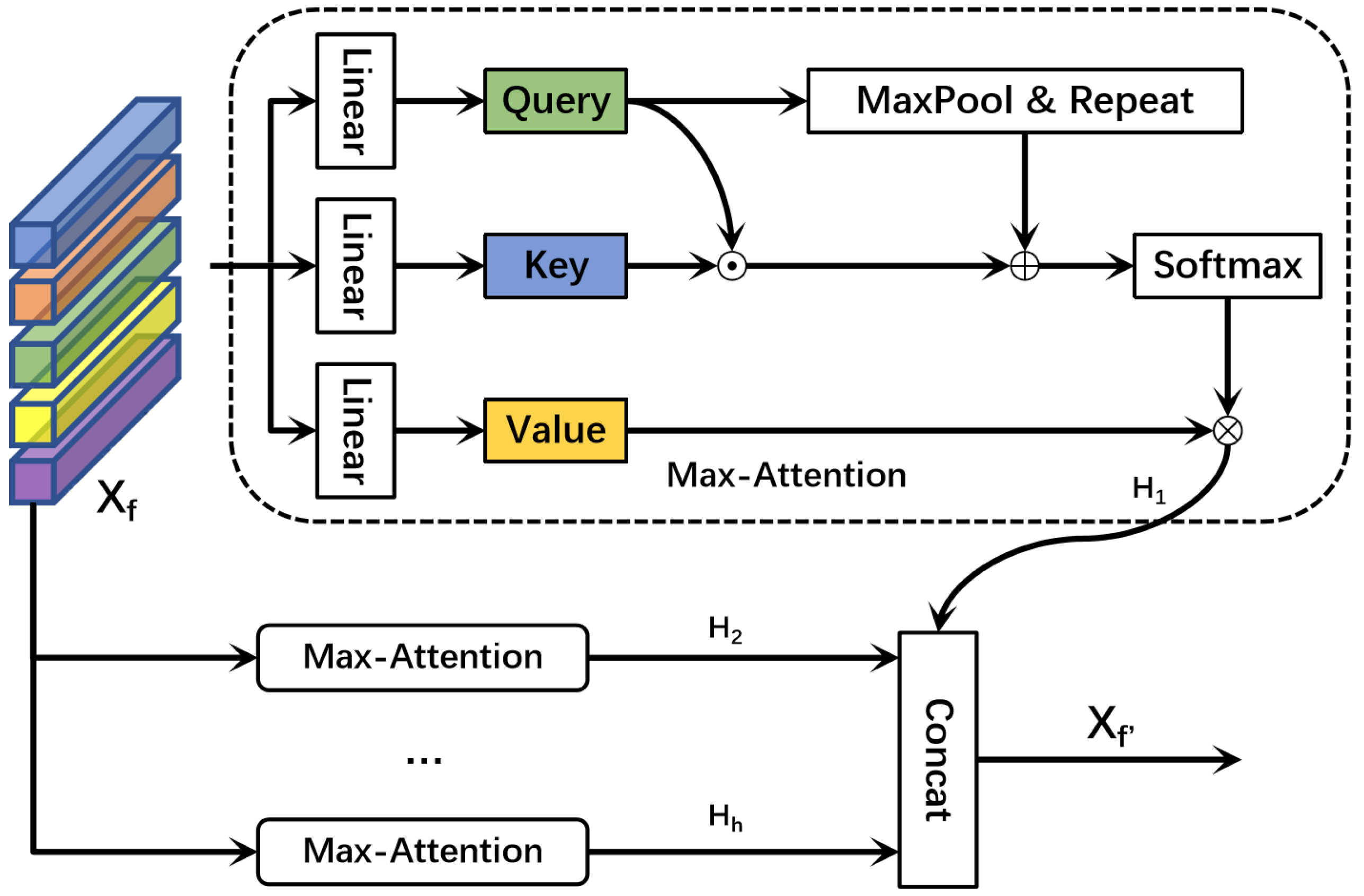
3.2. SFDM
3.2.1. Feature Fusion Module
3.2.2. Feature Enhancement Module
3.3. LSDM
3.3.1. Overview of GCN
3.3.2. Construction of a Correlation Matrix
3.3.3. Global Relationship Enhancement Module
4. Experiments
4.1. Evaluation Metrics
4.2. Implementation Details
4.3. Baseline Model Parameters
4.4. Experimental Results
4.4.1. Comparisons with State-of-the-Art Methods
4.4.2. Statistical Significance Experiment
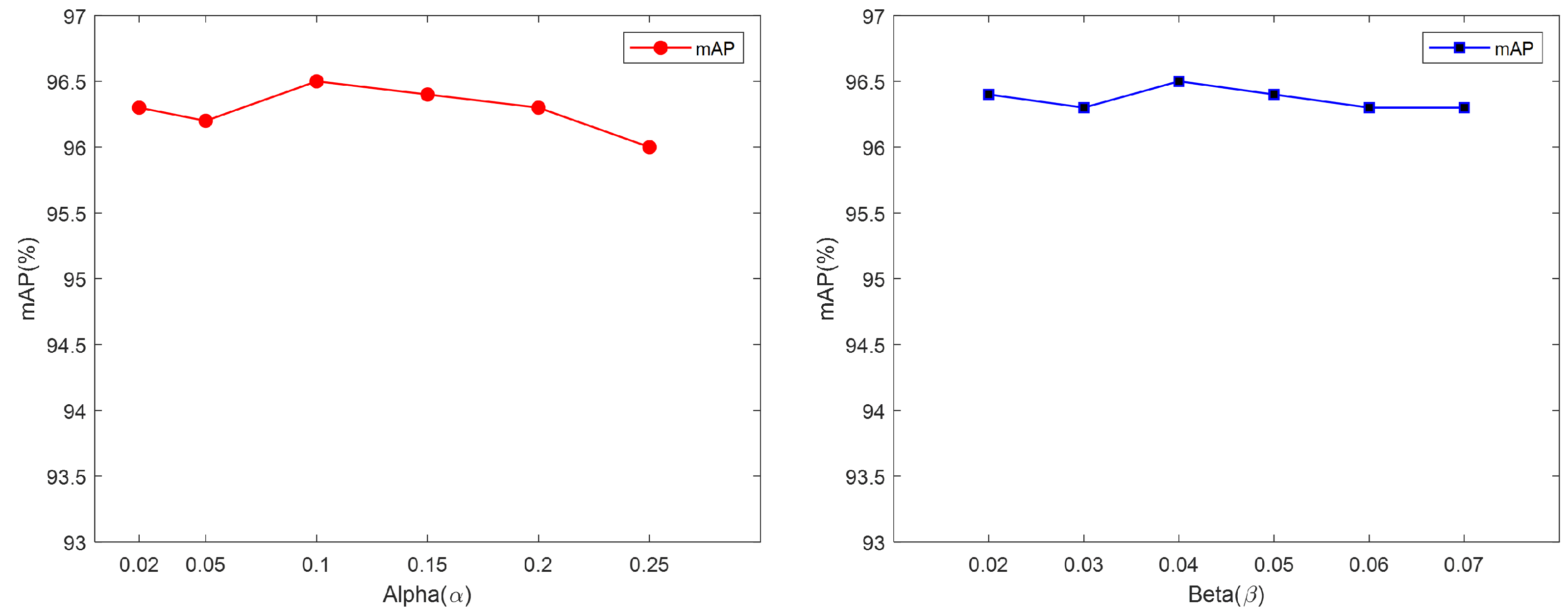
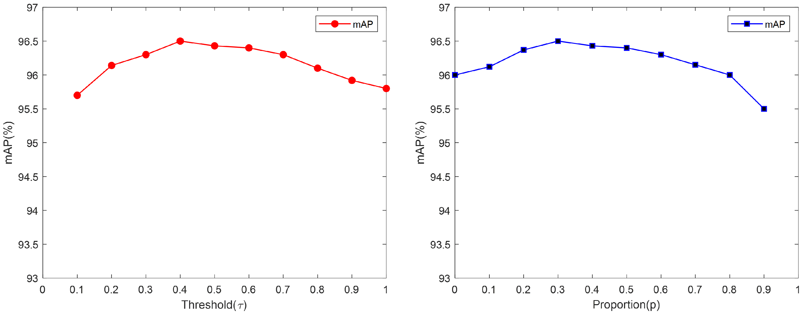
4.4.3. Ablation Studies
4.4.4. Computational Cost Analysis
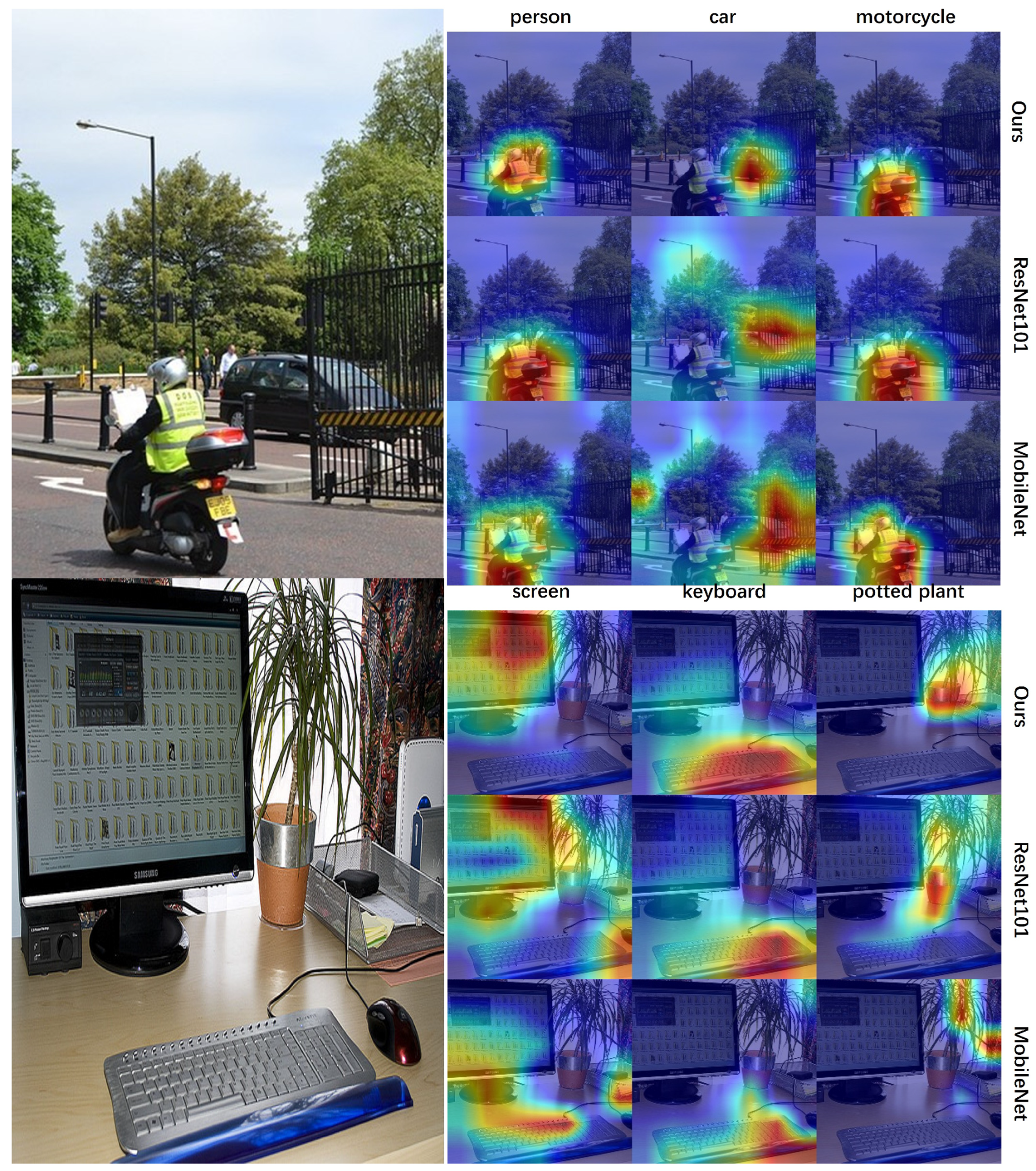
4.5. Visualization
5. Conclusions and Future Work
Author Contributions
Funding
Institutional Review Board Statement
Informed Consent Statement
Data Availability Statement
Acknowledgments
Conflicts of Interest
References
- Liu, C.; Meng, Z. TBFF-DAC: Two-branch feature fusion based on deformable attention and convolution for object detection. Comput. Electr. Eng. 2024, 116, 109132. [Google Scholar] [CrossRef]
- Sirisha, M.; Sudha, S. TOD-Net: An end-to-end transformer-based object detection network. Comput. Electr. Eng. 2023, 108, 108695. [Google Scholar] [CrossRef]
- Zhou, J.; Hu, Y.; Lai, Z.; Wang, T. SEGANet: 3D object detection with shape-enhancement and geometry-aware network. Comput. Electr. Eng. 2023, 110, 108888. [Google Scholar] [CrossRef]
- Vankdothu, R.; Hameed, M.A. Adaptive features selection and EDNN based brain image recognition on the internet of medical things. Comput. Electr. Eng. 2022, 103, 108338. [Google Scholar] [CrossRef]
- Mouzai, M.; Mustapha, A.; Bousmina, Z.; Keskas, I.; Farhi, F. Xray-Net: Self-supervised pixel stretching approach to improve low-contrast medical imaging. Comput. Electr. Eng. 2023, 110, 108859. [Google Scholar] [CrossRef]
- Ke, J.; Wang, W.; Chen, X.; Gou, J.; Gao, Y.; Jin, S. Medical entity recognition and knowledge map relationship analysis of Chinese EMRs based on improved BiLSTM-CRF. Comput. Electr. Eng. 2023, 108, 108709. [Google Scholar] [CrossRef]
- Ding, I.J.; Liu, J.T. Three-layered hierarchical scheme with a Kinect sensor microphone array for audio-based human behavior recognition. Comput. Electr. Eng. 2016, 49, 173–183. [Google Scholar] [CrossRef]
- Saw, C.Y.; Wong, Y.C. Neuromorphic computing with hybrid CNN–Stochastic Reservoir for time series WiFi based human activity recognition. Comput. Electr. Eng. 2023, 111, 108917. [Google Scholar] [CrossRef]
- Bharathi, A.; Sridevi, M. Human action recognition in complex live videos using graph convolutional network. Comput. Electr. Eng. 2023, 110, 108844. [Google Scholar] [CrossRef]
- Gao, B.B.; Zhou, H.Y. Learning to Discover Multi-Class Attentional Regions for Multi-Label Image Recognition. IEEE Trans. Image Process. 2021, 30, 5920–5932. [Google Scholar] [CrossRef]
- Liu, L.; Guo, S.; Huang, W.; Scott, M.R. Decoupling category-wise independence and relevance with self-attention for multi-label image classification. In Proceedings of the ICASSP 2019–2019 IEEE International Conference on Acoustics, Speech and Signal Processing (ICASSP), Brighton, UK, 12–17 May 2019; IEEE: Piscataway, NJ, USA, 2019; pp. 1682–1686. [Google Scholar]
- Chen, Z.M.; Wei, X.S.; Wang, P.; Guo, Y. Multi-label image recognition with graph convolutional networks. In Proceedings of the IEEE/CVF Conference on Computer Vision and Pattern Recognition, Long Beach, CA, USA, 15–20 June 2019; pp. 5177–5186. [Google Scholar]
- Liang, J.; Xu, F.; Yu, S. A multi-scale semantic attention representation for multi-label image recognition with graph networks. Neurocomputing 2022, 491, 14–23. [Google Scholar] [CrossRef]
- Chen, T.; Xu, M.; Hui, X.; Wu, H.; Lin, L. Learning semantic-specific graph representation for multi-label image recognition. In Proceedings of the IEEE/CVF International Conference on Computer Vision, Seoul, Republic of Korea, 27 October–2 November 2019; pp. 522–531. [Google Scholar]
- Girshick, R. Fast R-CNN. In Proceedings of the IEEE International Conference on Computer Vision, Santiago, Chile, 7–13 December 2015; pp. 1440–1448. [Google Scholar]
- Wang, Z.; Chen, T.; Li, G.; Xu, R.; Lin, L. Multi-label Image Recognition by Recurrently Discovering Attentional Regions. In Proceedings of the IEEE International Conference on Computer Vision, Venice, Italy, 22–29 October 2017. [Google Scholar]
- Li, X.; Zhao, F.; Guo, Y. Multi-label Image Classification with A Probabilistic Label Enhancement Model. In Proceedings of the UAI, Quebec City, QC, Canada, 23–27 July 2014; Volume 1, pp. 1–10. [Google Scholar]
- Wang, Y.; Xie, Y.; Zeng, J.; Wang, H.; Fan, L.; Song, Y. Cross-modal fusion for multi-label image classification with attention mechanism. Comput. Electr. Eng. 2022, 101, 108002. [Google Scholar] [CrossRef]
- Zhao, J.; Yan, K.; Zhao, Y.; Guo, X.; Huang, F.; Li, J. Transformer-based dual relation graph for multi-label image recognition. In Proceedings of the IEEE/CVF International Conference on Computer Vision, Montreal, BC, Canada, 11–17 October 2021; pp. 163–172. [Google Scholar]
- Zhang, M.; Zhou, Z. A Review on Multi-Label Learning Algorithms. IEEE Trans. Knowl. Data Eng. 2014, 26, 1819–1837. [Google Scholar] [CrossRef]
- Bogatinovski, J.; Todorovski, L.; Džeroski, S.; Kocev, D. Comprehensive comparative study of multi-label classification methods. Expert Syst. Appl. 2022, 203, 117215. [Google Scholar] [CrossRef]
- Tsoumakas, G.; Katakis, I. Multi-Label Classification: An Overview. Int. J. Data Warehous. Min. 2009, 3, 64–74. [Google Scholar]
- Lin, T.Y.; Maire, M.; Belongie, S.; Hays, J.; Perona, P.; Ramanan, D.; Dollár, P.; Zitnick, C.L. Microsoft COCO: Common Objects in Context. In Proceedings of the Computer Vision—ECCV 2014, Zurich, Switzerland, 6–12 September 2014; pp. 740–755. [Google Scholar]
- Everingham, M.; Van Gool, L.; Williams, C.K.; Winn, J.; Zisserman, A. The pascal visual object classes (voc) challenge. Int. J. Comput. Vis. 2010, 88, 303–338. [Google Scholar] [CrossRef]
- Deng, J.; Dong, W.; Socher, R.; Li, L.J.; Li, K.; Li, F. Imagenet: A large-scale hierarchical image database. In Proceedings of the 2009 IEEE Conference on Computer Vision and Pattern Recognition, Miami, FL, USA, 20–25 June 2009; IEEE: Piscataway, NJ, USA, 2009; pp. 248–255. [Google Scholar]
- He, K.; Zhang, X.; Ren, S.; Sun, J. Deep residual learning for image recognition. In Proceedings of the IEEE Conference on Computer Vision and Pattern Recognition, Las Vegas, NV, USA, 27–30 June 2016; pp. 770–778. [Google Scholar]
- Hu, J.; Shen, L.; Albanie, S.; Sun, G.; Wu, E. Squeeze-and-Excitation Networks. IEEE Trans. Pattern Anal. Mach. Intell. 2019, 99, 7132–7141. [Google Scholar]
- Rifkin, R.; Klautau, A. In defense of one-vs-all classification. J. Mach. Learn. Res. 2004, 5, 101–141. [Google Scholar]
- Zhang, M.L.; Li, Y.K.; Liu, X.Y.; Geng, X. Binary relevance for multi-label learning: An overview. Front. Comput. Sci. 2018, 12, 191–202. [Google Scholar] [CrossRef]
- Agrawal, R.; Srikant, R. Fast algorithms for mining association rules. In Proceedings of the 20th International Conference on Very Large Data Bases, VLDB, Santiago, Chile, 12–15 September 1994; Volume 1215, pp. 487–499. [Google Scholar]
- Han, J.; Pei, J.; Yin, Y. Mining frequent patterns without candidate generation. ACM Sigmod Rec. 2000, 29, 1–12. [Google Scholar] [CrossRef]
- Chen, Y.L.; Hsu, C.L.; Chou, S.C. Constructing a multi-valued and multi-labeled decision tree. Expert Syst. Appl. 2003, 25, 199–209. [Google Scholar] [CrossRef]
- Schapire, R.E.; Singer, Y. BoosTexter: A Boosting-based System for Text Categorization. Mach. Learn. 2000, 39, 135–168. [Google Scholar] [CrossRef]
- Zhang, M.L.; Zhou, Z.H. Multilabel Neural Networks with Applications to Functional Genomics and Text Categorization. IEEE Trans. Knowl. Data Eng. 2006, 18, 1338–1351. [Google Scholar] [CrossRef]
- Chollet, F. Xception: Deep learning with depthwise separable convolutions. In Proceedings of the IEEE Conference on Computer Vision and Pattern Recognition, Honolulu, HI, USA, 21–26 July 2017; pp. 1251–1258. [Google Scholar]
- Xie, S.; Girshick, R.; Dollár, P.; Tu, Z.; He, K. Aggregated Residual Transformations for Deep Neural Networks. In Proceedings of the IEEE Conference on Computer Vision and Pattern Recognition, Las Vegas, NV, USA, 27–30 July 2016. [Google Scholar]
- Zhang, X.; Zhou, X.; Lin, M.; Sun, J. Shufflenet: An extremely efficient convolutional neural network for mobile devices. In Proceedings of the IEEE Conference on Computer Vision and Pattern Recognition, Salt Lake City, UT, USA, 18–23 June 2018; pp. 6848–6856. [Google Scholar]
- Cheng, M.M.; Zhang, Z.; Lin, W.Y.; Torr, P. BING: Binarized normed gradients for objectness estimation at 300 fps. In Proceedings of the IEEE Conference on Computer Vision and Pattern Recognition, Columbus, OH, USA, 23–28 June 2014; pp. 3286–3293. [Google Scholar]
- Wang, J.; Yang, Y.; Mao, J.; Huang, Z.; Huang, C.; Xu, W. Cnn-rnn: A unified framework for multi-label image classification. In Proceedings of the IEEE Conference on Computer Vision and Pattern Recognition, Las Vegas, NV, USA, 27–30 June 2016; pp. 2285–2294. [Google Scholar]
- Feng, Z.; Li, H.; Ouyang, W.; Yu, N.; Wang, X. Learning Spatial Regularization with Image-Level Supervisions for Multi-label Image Classification. In Proceedings of the IEEE Conference on Computer Vision and Pattern Recognition, Honolulu, HI, USA, 21–26 July 2017; IEEE: Piscataway, NJ, USA, 2017. [Google Scholar]
- Lin, R.; Xiao, J.; Fan, J. Nextvlad: An efficient neural network to aggregate frame-level features for large-scale video classification. In Proceedings of the European Conference on Computer Vision (ECCV) Workshops, Munich, Germany, 8–14 September 2018; pp. 206–218. [Google Scholar]
- Guo, H.; Zheng, K.; Fan, X.; Yu, H.; Wang, S. Visual attention consistency under image transforms for multi-label image classification. In Proceedings of the IEEE/CVF Conference on Computer Vision and Pattern Recognition, Long Beach, CA, USA, 15–20 June 2019; pp. 729–739. [Google Scholar]
- Hand, E.; Castillo, C.; Chellappa, R. Doing the best we can with what we have: Multi-label balancing with selective learning for attribute prediction. In Proceedings of the AAAI Conference on Artificial Intelligence, New Orleans, LA, USA, 2–7 February 2018; Volume 32. [Google Scholar]
- Li, Q.; Qiao, M.; Bian, W.; Tao, D. Conditional graphical lasso for multi-label image classification. In Proceedings of the IEEE Conference on Computer Vision and Pattern Recognition, Las Vegas, NV, USA, 27–30 June 2016; pp. 2977–2986. [Google Scholar]
- Ye, J.; He, J.; Peng, X.; Wu, W.; Qiao, Y. Attention-driven dynamic graph convolutional network for multi-label image recognition. In Computer Vision–ECCV 2020: Proceedings of the 16th European Conference, Glasgow, UK, 23–28 August 2020; Proceedings, Part XXI 16; Springer: Berlin/Heidelberg, Germany, 2020; pp. 649–665. [Google Scholar]
- Cao, P.; Chen, P.; Niu, Q. Multi-label image recognition with two-stream dynamic graph convolution networks. Image Vis. Comput. 2021, 113, 104238. [Google Scholar] [CrossRef]
- Dao, S.D.; Zhao, H.; Phung, D.; Cai, J. Contrastively enforcing distinctiveness for multi-label image classification. Neurocomputing 2023, 555, 126605. [Google Scholar] [CrossRef]
- Deng, X.; Feng, S.; Lyu, G.; Wang, T.; Lang, C. Beyond Word Embeddings: Heterogeneous Prior Knowledge Driven Multi-Label Image Classification. IEEE Trans. Multimed. 2023, 25, 4013–4025. [Google Scholar] [CrossRef]
- Chen, Y.; Zou, C.; Chen, J. Label-aware graph representation learning for multi-label image classification. Neurocomputing 2022, 492, 50–61. [Google Scholar] [CrossRef]
- Yang, H.; Zhou, T.; Zhang, Y.; Gao, B.B.; Wu, J.; Cai, J. Exploit bounding box annotations for multi-label object recognition. In Proceedings of the IEEE Conference on Computer Vision and Pattern Recognition, Las Vegas, NV, USA, 27–30 June 2016; pp. 280–288. [Google Scholar]
- Chen, T.; Wang, Z.; Li, G.; Lin, L. Recurrent attentional reinforcement learning for multi-label image recognition. In Proceedings of the AAAI Conference on Artificial Intelligence, New Orleans, LA, USA, 2–7 February 2018; Volume 32. [Google Scholar]
- Nie, L.; Chen, T.; Wang, Z.; Kang, W.; Lin, L. Multi-label image recognition with attentive transformer-localizer module. Multimed. Tools Appl. 2022, 81, 7917–7940. [Google Scholar] [CrossRef]
- Sun, D.; Ma, L.; Ding, Z.; Luo, B. An attention-driven multi-label image classification with semantic embedding and graph convolutional networks. Cogn. Comput. 2022, 15, 1308–1319. [Google Scholar] [CrossRef]
- Wei, Y.; Xia, W.; Lin, M.; Huang, J.; Ni, B.; Dong, J.; Zhao, Y.; Yan, S. HCP: A flexible CNN framework for multi-label image classification. IEEE Trans. Pattern Anal. Mach. Intell. 2015, 38, 1901–1907. [Google Scholar] [CrossRef]
- Wang, M.; Luo, C.; Hong, R.; Tang, J.; Feng, J. Beyond Object Proposals: Random Crop Pooling for Multi-Label Image Recognition. IEEE Trans. Image Process. 2016, 25, 5678–5688. [Google Scholar] [CrossRef] [PubMed]
- Xie, Y.; Wang, Y.; Liu, Y.; Zhou, K. Label graph learning for multi-label image recognition with cross-modal fusion. Multimed. Tools Appl. 2022, 81, 25363–25381. [Google Scholar] [CrossRef]
- Wang, Y.; Xie, Y.; Fan, L.; Hu, G. STMG: Swin transformer for multi-label image recognition with graph convolution network. Neural Comput. Appl. 2022, 34, 10051–10063. [Google Scholar] [CrossRef]


| Methods | Aero | Bike | Bird | Boat | Bot | Bus | Car | Cat | Chair | Cow | Table | Dog | Horse | Mot | Pers | Plant | Sheep | Sofa | Train | Tv | mAP |
|---|---|---|---|---|---|---|---|---|---|---|---|---|---|---|---|---|---|---|---|---|---|
| CNN-RNN [39] | 96.7 | 83.1 | 94.2 | 92.8 | 61.2 | 82.1 | 89.1 | 94.2 | 64.2 | 83.6 | 70.0 | 92.4 | 91.7 | 84.2 | 93.7 | 59.8 | 93.2 | 75.3 | 99.7 | 78.6 | 84.0 |
| ResNet-101 [26] | 99.5 | 97.7 | 97.8 | 96.4 | 65.7 | 91.8 | 96.1 | 97.6 | 74.2 | 80.9 | 85.0 | 98.4 | 96.5 | 95.9 | 98.4 | 70.1 | 88.3 | 80.2 | 98.9 | 89.2 | 89.9 |
| FeV+LV [50] | 97.9 | 97.0 | 96.6 | 94.6 | 73.6 | 93.9 | 96.5 | 95.5 | 73.7 | 90.3 | 82.8 | 95.4 | 97.7 | 95.9 | 98.6 | 77.6 | 88.7 | 78.0 | 98.3 | 89.0 | 90.6 |
| Atten-Reinforce [51] | 98.6 | 97.1 | 97.1 | 95.5 | 75.6 | 92.8 | 96.8 | 97.3 | 78.3 | 92.2 | 87.6 | 96.9 | 96.5 | 93.6 | 98.5 | 81.6 | 93.1 | 83.2 | 98.5 | 89.3 | 92.0 |
| ATL [52] | 99.0 | 97.2 | 96.6 | 96.2 | 75.4 | 92.0 | 96.8 | 97.2 | 79.0 | 93.6 | 89.3 | 97.0 | 97.5 | 94.0 | 98.8 | 81.6 | 94.3 | 85.8 | 98.7 | 90.6 | 92.5 |
| ML-GCN [12] | 99.5 | 98.5 | 98.6 | 98.1 | 80.8 | 94.6 | 97.2 | 98.2 | 82.3 | 95.7 | 86.4 | 98.2 | 98.4 | 96.7 | 99.0 | 84.7 | 96.7 | 84.3 | 98.9 | 93.7 | 94.0 |
| GCN-MS-SGA [13] | 99.6 | 98.3 | 98.0 | 97.5 | 81.0 | 93.1 | 97.5 | 98.5 | 86.3 | 88.3 | 89.2 | 95.5 | 98.0 | 96.1 | 98.3 | 89.0 | 96.7 | 91.6 | 97.9 | 92.3 | 94.2 |
| LGR [49] | 99.6 | 95.6 | 97.3 | 96.4 | 84.0 | 95.8 | 94.1 | 98.9 | 86.9 | 96.8 | 86.8 | 98.7 | 98.6 | 96.9 | 98.8 | 84.8 | 97.2 | 83.7 | 98.8 | 93.6 | 94.2 |
| FLNet [53] | 99.6 | 98.7 | 98.9 | 97.9 | 84.6 | 95.3 | 96.2 | 96.5 | 85.6 | 96.1 | 87.2 | 97.7 | 98.6 | 97.0 | 98.1 | 86.5 | 97.4 | 86.5 | 98.8 | 90.8 | 94.4 |
| CFMIC [18] | 99.7 | 98.5 | 98.8 | 98.3 | 83.9 | 96.5 | 97.5 | 98.8 | 83.1 | 96.1 | 87.4 | 98.6 | 98.9 | 97.2 | 99.0 | 85.4 | 97.1 | 84.9 | 99.2 | 94.2 | 94.7 |
| SSGRL [14] | 99.7 | 98.4 | 98.0 | 97.6 | 85.7 | 96.2 | 98.2 | 98.8 | 82.0 | 98.1 | 89.7 | 98.8 | 98.7 | 97.0 | 99.0 | 86.9 | 98.1 | 85.8 | 99.0 | 93.7 | 95.0 |
| VSGCN [48] | 99.8 | 98.6 | 98.7 | 98.6 | 85.2 | 96.9 | 98.2 | 98.6 | 83.6 | 96.5 | 87.8 | 99.1 | 99.0 | 97.5 | 99.3 | 85.8 | 96.3 | 87.6 | 98.6 | 95.2 | 95.1 |
| MulCon [47] | 99.8 | 98.3 | 99.3 | 98.6 | 83.3 | 98.4 | 98.0 | 98.3 | 85.8 | 98.3 | 90.5 | 99.3 | 98.9 | 96.6 | 98.8 | 86.3 | 99.8 | 87.3 | 99.8 | 96.1 | 95.6 |
| Ours | 99.6 | 99.1 | 98.8 | 98.9 | 85.8 | 97.9 | 98.5 | 99.1 | 87.9 | 98.1 | 92.9 | 99.1 | 98.6 | 98.6 | 99.3 | 90.9 | 98.8 | 91.3 | 99.8 | 97.0 | 96.5 |
| Methods | Aero | Bike | Bird | Boat | Bot | Bus | Car | Cat | Chair | Cow | Table | Dog | Horse | Mot | Pers | Plant | Sheep | Sofa | Train | Tv | mAP |
|---|---|---|---|---|---|---|---|---|---|---|---|---|---|---|---|---|---|---|---|---|---|
| Fev+Lv [50] | 98.4 | 92.8 | 93.4 | 90.7 | 74.9 | 93.2 | 90.2 | 96.1 | 78.2 | 89.8 | 80.6 | 95.7 | 96.1 | 95.3 | 97.5 | 73.1 | 91.2 | 75.4 | 97.0 | 88.2 | 89.4 |
| HCP [54] | 99.1 | 92.8 | 97.4 | 94.4 | 79.9 | 93.6 | 89.8 | 98.2 | 78.2 | 94.9 | 79.8 | 97.8 | 97.0 | 93.8 | 96.4 | 74.3 | 94.7 | 71.9 | 96.7 | 88.6 | 90.5 |
| RCP [55] | 99.3 | 92.2 | 97.5 | 94.9 | 82.3 | 94.1 | 92.4 | 98.5 | 83.8 | 93.5 | 83.1 | 98.1 | 97.3 | 96.0 | 98.8 | 77.7 | 95.1 | 79.4 | 97.7 | 92.4 | 92.2 |
| MCAR [10] | 99.6 | 97.1 | 98.3 | 96.6 | 87.0 | 95.5 | 94.4 | 98.8 | 87.0 | 96.9 | 85.0 | 98.7 | 98.3 | 97.3 | 99.0 | 83.8 | 96.8 | 83.7 | 98.3 | 93.5 | 94.3 |
| SSGRL [14] | 99.7 | 96.1 | 97.7 | 96.5 | 86.9 | 95.8 | 95.0 | 98.9 | 88.3 | 97.6 | 87.4 | 99.1 | 99.2 | 97.3 | 99.0 | 84.8 | 98.3 | 85.8 | 99.2 | 94.1 | 94.8 |
| Ours | 99.7 | 97.5 | 99.0 | 97.6 | 87.1 | 97.7 | 96.2 | 99.7 | 90.2 | 98.4 | 89.3 | 99.1 | 99.3 | 97.4 | 99.0 | 88.0 | 99.1 | 88.5 | 99.7 | 97.3 | 96.0 |
| Methods | ALL | TOP-3 | |||||||||||
|---|---|---|---|---|---|---|---|---|---|---|---|---|---|
| mAP | CP | CR | CF1 | OP | OR | OF1 | CP | CR | CF1 | OP | OR | OF1 | |
| CNN-RNN [39] | 61.2 | - | - | - | - | - | - | 66.0 | 55.6 | 66.4 | 69.2 | 66.4 | 67.8 |
| SRN [40] | 77.1 | 81.6 | 65.4 | 71.2 | 82.7 | 69.9 | 75.8 | 85.2 | 58.8 | 67.4 | 87.4 | 62.5 | 72.9 |
| ResNet-101 [26] | 77.3 | 80.2 | 66.7 | 72.8 | 83.9 | 70.8 | 76.8 | 84.1 | 59.4 | 69.7 | 89.1 | 62.8 | 73.6 |
| ML-GCN [12] | 83.0 | 85.1 | 72.0 | 78.0 | 85.8 | 75.4 | 80.3 | 89.2 | 64.1 | 74.6 | 90.5 | 66.5 | 76.7 |
| GCN-MS-SGA [13] | 83.4 | 85.1 | 71.6 | 77.8 | 84.0 | 75.0 | 79.3 | 88.8 | 63.4 | 75.7 | 88.8 | 66.0 | 75.7 |
| MCAR [10] | 83.8 | 85.0 | 72.1 | 78.0 | 88.0 | 73.9 | 80.3 | 88.1 | 65.5 | 75.1 | 91.0 | 66.3 | 76.7 |
| CFMIC [18] | 83.8 | 85.8 | 72.7 | 78.7 | 86.3 | 76.3 | 81.0 | 89.7 | 64.5 | 75.0 | 90.7 | 67.3 | 77.3 |
| LGR [49] | 83.9 | 85.0 | 73.3 | 78.7 | 86.2 | 76.4 | 81.0 | 89.0 | 64.8 | 75.0 | 90.7 | 67.0 | 77.1 |
| FLNet [53] | 84.1 | 84.9 | 73.9 | 79.0 | 85.5 | 77.4 | 81.1 | 89.0 | 65.2 | 75.2 | 90.4 | 67.5 | 77.3 |
| LGLM [56] | 84.2 | 85.7 | 72.8 | 78.7 | 86.6 | 76.7 | 81.3 | 89.4 | 64.7 | 75.0 | 90.7 | 67.4 | 77.3 |
| STMG [57] | 84.3 | 85.8 | 72.7 | 78.7 | 86.7 | 76.8 | 81.5 | 89.3 | 64.8 | 75.1 | 90.8 | 67.4 | 77.4 |
| Ours | 85.2 | 84.1 | 75.9 | 79.8 | 85.2 | 78.7 | 81.8 | 88.7 | 66.5 | 76.0 | 90.5 | 68.1 | 77.7 |
| Methods | CNN-RNN [39] | ResNet-101 [26] | FeV+LV [50] | Atten-Reinforce [51] | ATL [52] | ML-GCN [12] | GCN-MS-SGA [13] | LGR [49] | FLNet [53] | CFMIC [18] | SSGRL [14] | VSGCN [48] | MulCon [47] |
|---|---|---|---|---|---|---|---|---|---|---|---|---|---|
| p-value | |||||||||||||
| Confidence interval | [8.52, 16.50] | [3.38, 9.76] | [3.72, 8.12] | [3.03, 5.96] | [2.57, 5.37] | [1.38, 3.57] | [1.26, 3.41] | [1.30, 3.37] | [1.24, 2.96] | [0.88, 2.81] | [0.66, 2.40] | [0.63, 2.28] | [0.21, 1.64] |
| SFDM | LSDM | mAP | ||
|---|---|---|---|---|
| FFM | FEM | GCN | GREM | |
| ✔ | ✔ | ✔ | ✔ | 96.5 |
| ✔ | ✔ | 95.0 | ||
| ✔ | ✔ | 94.3 | ||
| ✔ | ✔ | ✔ | 94.9 | |
| ✔ | ✔ | ✔ | 94.6 | |
| ✔ | ✔ | ✔ | 95.7 | |
| Modules | LSDM | SFDM | FFM | FEM | GREM |
|---|---|---|---|---|---|
| p-value |
| Methods | All | ||
|---|---|---|---|
| mAP | OF1 | CF1 | |
| add()add() | 94.8 | 92.2 | 90.5 |
| mul()add() | 96.3 | 93.2 | 92.0 |
| mul()mul() | 95.5 | 93.0 | 91.6 |
| add()mul() | 96.5 | 93.2 | 92.2 |
Disclaimer/Publisher’s Note: The statements, opinions and data contained in all publications are solely those of the individual author(s) and contributor(s) and not of MDPI and/or the editor(s). MDPI and/or the editor(s) disclaim responsibility for any injury to people or property resulting from any ideas, methods, instructions or products referred to in the content. |
© 2025 by the authors. Licensee MDPI, Basel, Switzerland. This article is an open access article distributed under the terms and conditions of the Creative Commons Attribution (CC BY) license (https://creativecommons.org/licenses/by/4.0/).
Share and Cite
Wang, J.; Zhang, Y.; Wang, T.; Tang, H.; Li, B. Establishing Two-Dimensional Dependencies for Multi-Label Image Classification. Appl. Sci. 2025, 15, 2845. https://doi.org/10.3390/app15052845
Wang J, Zhang Y, Wang T, Tang H, Li B. Establishing Two-Dimensional Dependencies for Multi-Label Image Classification. Applied Sciences. 2025; 15(5):2845. https://doi.org/10.3390/app15052845
Chicago/Turabian StyleWang, Jiuhang, Yuewen Zhang, Tengjing Wang, Hongying Tang, and Baoqing Li. 2025. "Establishing Two-Dimensional Dependencies for Multi-Label Image Classification" Applied Sciences 15, no. 5: 2845. https://doi.org/10.3390/app15052845
APA StyleWang, J., Zhang, Y., Wang, T., Tang, H., & Li, B. (2025). Establishing Two-Dimensional Dependencies for Multi-Label Image Classification. Applied Sciences, 15(5), 2845. https://doi.org/10.3390/app15052845