AsGCL: Attentive and Simple Graph Contrastive Learning for Recommendation

Abstract

In contemporary society, individuals are inundated with a vast amount of redundant information, and recommendation systems have undoubtedly opened up new avenues for managing irrelevant data. Graph convolutional networks (GCNs) have demonstrated remarkable performance in the field of recommendation systems by iteratively performing node convolutions to capture information from neighboring nodes, thereby enhancing recommendation efficacy. However, most existing models fail to distinguish the importance of different nodes, which limits their performance. To address this issue, we propose the asGCL model. To mitigate the prevalent issue of popularity bias and to learn more uniform embedding representations, we have integrated a lightweight contrastive learning module into our model. Finally, extensive experiments conducted on four real-world datasets demonstrate the effectiveness of our model. Notably, on the Amazon-Books dataset, our asGCL model achieved improvements of 4.21% and 8.74% in recall@20 and NDCG@20, respectively.

1. Introduction

Since its inception, recommendation systems have been widely implemented across various social platforms, alleviating users from much of the decision-making burden associated with selecting products or obtaining information. With the support of deep learning, recommendation models are capable of learning more valuable item content from users’ historical evaluations and behaviors. This capability represents one of the most practical and valuable directions in the current landscape of model development.

Collaborative filtering methods [1,2] are among the most classic algorithms in recommendation systems. They construct a co-occurrence matrix with users represented on the horizontal axis and items on the vertical axis, calculating the similarity between pairs of columns and ranking them based on similarity scores. While collaborative filtering is an intuitive and highly interpretable algorithm, it suffers from a lack of generalization capability and is unable to effectively address the pervasive issue of sparse matrices. Consequently, matrix factorization techniques [3] have emerged, generating corresponding latent vectors for each user and item, thereby reducing the dimensionality of the co-occurrence matrix and uncovering hidden interest information. This approach aligns closely with the embedding concepts in deep learning, allowing matrix factorization to extend beyond interaction information and to be combined with other features, thereby opening the door to deep learning applications.

Whether it is collaborative filtering, matrix factorization, or deep recommendation models [4,5], the encoding of target nodes typically remains in the first order, focusing only on the immediate neighbors of the target node. This approach often lacks a more precise encoding of the collaborative signals between users and items, which is crucial for revealing the similarities between embedding vectors. When the embedding representations fail to capture deeper interaction knowledge, we need to rely on effective interaction functions to compensate for the shortcomings of suboptimal embeddings.

As a result, graph convolutional network (GCN) [6] recommendation methods have begun to gain traction. Taking social networks as an example, users are represented as nodes, and the relationships between users are represented as edges, forming a graph structure. These methods recursively propagate embedding signals across the interaction graph and model the information of multi-hop neighbor nodes through interaction functions. Specifically, high-order connectivity refers to any path with a length greater than 1 that reaches the target node, encapsulating rich semantic and collaborative signals. Models based on graph neural networks (GNNs) offer enhanced embedding expressiveness and interpretability, making them a powerful tool for recommendation tasks.

We observe that models based on graph neural networks do not differentiate between the input nodes; however, the initial input nodes inherently possess varying degrees of importance. Specifically, nodes with higher degrees of correlation should be assigned superior values to facilitate differentiation. On the other hand, to mitigate the issue of popularity bias, contrastive learning typically aims to achieve this goal by learning more uniform and homogeneous embedding representations. Therefore, our proposed asGCL model addresses this problem from two perspectives: first, by calculating the weights of the nodes, and second, by incorporating a contrastive learning task.

In summary, our contributions are as follows:

• In this article, we provide a detailed analysis of the connections and distinctions between matrix factorization techniques and the input layer of graph convolutional networks, and we also adapt the attention mechanism from the field of computer vision to recommendation systems.
• We propose a novel graph collaborative filtering recommendation method, asGCL, in which the attention (ATT) module is utilized to compute node weights, and the very simple contrastive learning (SSCL) module is employed to enhance the representational capacity of the embeddings.
• Extensive experiments conducted on several real-world datasets demonstrate the effectiveness of asGCL. In-depth analyses further validate the model’s rationale and robustness.

2. Related Work

Neural Collaborative Filtering (NeuMF) [4] was the first to integrate multi-layer perceptrons (MLPs) with recommendation systems, establishing a dual network that separately models users and items with the aim of capturing their nonlinear relationships. Linear models excel at memorization, while Deep Neural Networks (DNNs) are proficient in generalization. The Deep Matrix Factorization (DeepFM) [5] model combines the advantages of both by integrating a linear regression model with a multi-layer fully connected network, and it replaces the linear regression component with Factorization Machines (FMs) to eliminate the need for manual feature interactions. The Deep Cross-Network (DCN) [7] further addresses the wide component by designing a specific cross-network that autonomously learns feature fusion information. xDeepFM [8] takes this a step further by constructing a Compressed Interaction Network (CIN) layer to learn high-order interaction features.

Graph neural networks (GNNs) [9,10] have revolutionized the data modeling approaches in recommendation systems, giving rise to models that have excelled across various scenarios, such as those discussed in references [11,12]. The graph convolutional network (GCN) innovatively introduces convolutional methods into the realm of recommendations, enabling multi-layer node aggregation operations that result in rich and interpretable graph embeddings. Such recommendation models continue to receive significant attention, exemplified by models like Neural Graph Collaborative Filtering (NGCF) [6], LightGCN [13], Liner Residual Graph Convolutional Network (LR-GCCF) [14], and Low-pass Collaborative Filtering (LCF) [15]. Notably, LightGCN has emerged as a foundational framework for numerous subsequent studies due to its simplicity and efficiency.

The graph convolutional network (GCN) faces challenges in assigning different learning weights to neighboring nodes, whereas the Graph Attention Network (GAT) excels in better integrating the correlations among vertex features into the model. The Attention-based Factorization Machine (AFM) [16] is one of the earlier works to introduce attention mechanisms into recommendation systems, positing that different cross-features exert varying influences on the outcomes. The Deep Interest Network (DIN) [17] proposes a mechanism that employs attention to compute user interest distributions for different items, effectively capturing the diversity of a user’s interests.

The self-supervised Hypergraph Convolutional Network (DHCN) [18] proposed a dual-channel hypergraph convolutional network for the social-based recommendation (SBR) task, marking the first time that the concept of self-supervised learning was integrated into the network training for recommendation tasks. The Multi-Channel Hypergraph Convolutional Network (MHCN) [12] combined multi-channel high-order user relationships with self-supervised learning, demonstrating that self-supervised auxiliary tasks can significantly enhance social recommendation performance. Self-supervised Graph Learning (SGL) [19] approached the problem from a graph structure perspective, designing three different types of data augmentation to construct auxiliary contrastive tasks. Neighborhood-enriched Contrastive Learning (NCL) [20] incorporated both graph structure contrastive tasks and semantic neighbor contrastive tasks into the main recommendation task for holistic training. LightGCL [21] posits that heuristic-based augmentation techniques for generating contrastive views do not effectively preserve the intrinsic semantic structure. Graph Contrastive Learning with Cohesive Subgraph Awareness [22] proposes a unified framework called CTAug, which seamlessly integrates cohesive subgraph awareness into existing graph contrastive learning mechanisms.

3. Preliminaries

3.1. Matrix Factorization (MF) and Graph Collaborative Filtering (GCF)

We conceptualize users and items as nodes in a bipartite graph, where users are connected to the items they have selected. Consequently, the task of identifying the optimal recommended items transforms into a link prediction problem [17]. Graph collaborative filtering is an embedding-based model [23,24], with matrix factorization being the most commonly used approach in traditional recommendation systems, demonstrating significant practical value. As a result, it has become a baseline model for many subsequent studies.

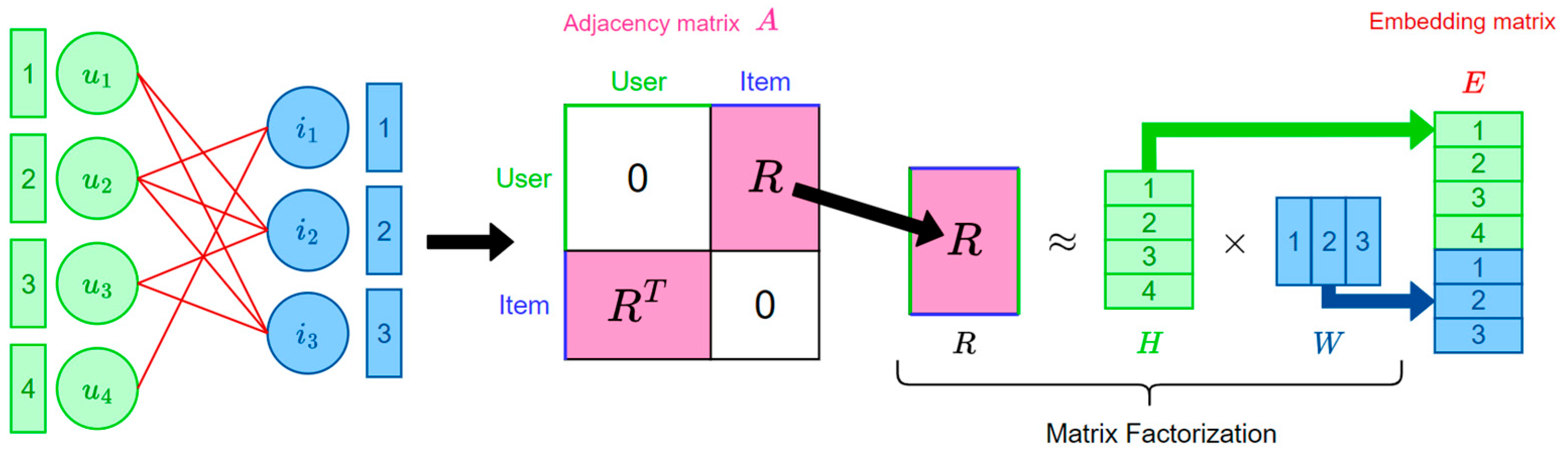
The Figure 1 illustrates the relationship between the matrix factorization process, the original graph, and the embedding matrices. Here, matrix R represents the user–item adjacency matrix, matrix $H$ contains user embeddings, and $W$ contains item embeddings. The user–item bipartite graph $\mathcal{G}=\left(\mathcal{V},A\right)$, where $\mathcal{V}=\mathcal{U}\cup \mathcal{I}$, has an adjacency matrix $A\in {ℝ}^{n\times n}$, which can be expressed as follows:

$$A=\left[\begin{array}{cc}{0}^{\left|\mathcal{U}\right|\times \left|\mathcal{U}\right|}& R\\ R^T& 0^{\left|\mathcal{I}\right|\times \left|\mathcal{I}\right|}\end{array}\right].$$

(1)

For the embedding vectors, users with similar preferences will have similar embeddings. Embedding-based models aim to find optimal embeddings for users and items. Typically, we need to compute the optimal scoring function $f$, where $f$ is the scalar product of the two embeddings. The model is trained by minimizing the Frobenius norm of the matrix $R-HW$.

3.2. LightGCN

The matrix factorization method described in the previous section has certain limitations, as it can only capture information from the direct neighbors of a given node in the graph. However, we aim to obtain information from multi-hop neighbor nodes, as this enhances the utilization of the graph structure. LightGCN [13] addresses this need.

LightGCN is derived from graph collaborative filtering (GCF) [6], but it differentiates itself by eliminating nonlinear activations and matrix transformations that have been shown to be less effective. This modification is likely due to the fact that in recommendation systems, each graph node is constructed and trained using only the IDs of users or items, resulting in less rich information compared to that found in image data.

LightGCN employs the embedding matrix from matrix factorization as the initial embedding and then completes the embedding training through three layers of embedding propagation. In each layer, each node updates its information by aggregating the embeddings of its neighbors, which can be conceptualized as a form of graph convolution [25]. The mathematical representation of this process is illustrated as shown in Figure 2.

In this context, $D$ represents a diagonal degree matrix, and $\tilde{A}=D^{-1/2}A{D}^{-1/2}$ is a diffusion matrix computed from the degree matrix $D$ and the adjacency matrix $A$, which only needs to be calculated once. This multi-layer embedding propagation process can be abstracted as follows:

$$e_u^{\left(k+1\right)}=AGG(e_u^{\left(k\right)},e_i^{\left(k\right)},i\in N_u\}).$$

(2)

The iterative aggregation formula for each layer is expressed as follows:

$$e_u^{\left(l+1\right)}={{\displaystyle \sum }}_{i\in N_u}{\displaystyle \frac{1}{\sqrt{\left|N_u\right|}\sqrt{\left|N_i\right|}}}{e}_i^{\left(l\right)} , e_i^{\left(l+1\right)}={{\displaystyle \sum }}_{u\in N_i}{\displaystyle \frac{1}{\sqrt{\left|N_i\right|}\sqrt{\left|N_u\right|}}}{e}_u^{\left(l\right)}.$$

(3)

In this model, the only learnable parameters are the initial embeddings. The final embeddings are obtained by summing the embeddings from each layer as follows:

$$e_u={{\displaystyle \sum }}_{k=0}^K{\alpha }_k{e}_u^k, e_i={{\displaystyle \sum }}_{k=0}^K{\alpha }_k{e}_i^k.$$

(4)

3.3. Attention Mechanism

Squeeze-and-Excitation Net (SENet) [26] is a novel network architecture proposed by the Momenta team led by Jue Hu, motivated by the desire to explicitly model the interdependencies among feature channels. Specifically, it aims to automatically learn the importance of each feature channel, thereby enhancing useful features while suppressing those that are less relevant to the current task.

To better integrate semantically and scale-inconsistent features, Dai et al. introduced the Multi-scale Channel Attention Module (MS-CAM) [27], which builds upon the concepts of SENet. This approach combines local and global features within a convolutional neural network (CNN) and utilizes attention mechanisms to spatially integrate multi-scale information.

However, as of now, SENet has not been implemented in the field of recommendation systems. In the domain of image processing, it pools each two-dimensional feature channel into a single real number, which possesses a global receptive field, and the output dimension corresponds to the number of input feature channels. Inspired by this, we note in Section 3.1 that the input to graph convolutional recommendation systems is an embedding matrix. We can treat this matrix as having only one-dimensional feature channels, pooling the embedding matrix into a real-valued vector. Subsequently, we can employ the attention mechanism from the fully connected layer of SENet to learn this set of real numbers. Ultimately, by multiplying the resulting set of invariant attention scores with the original embedding vector, we obtain a new embedding vector that is weighted accordingly.

3.4. Contrastive Learning

Graph recommendation systems based on contrastive learning [28] demonstrate significant advantages in both performance and robustness. The graph contrastive recommendation method represented by SGL employs strategies, such as sampling and edge dropout, to construct various perspectives of the user–item interaction graph. Thereby, it provides additional supervisory signals. Generally, the contrastive loss across different perspectives is computed to offer supplementary supervision to the primary recommendation task. This contrastive loss is defined as follows:

$${\mathrm{L}}_{cl}={{\displaystyle \sum }}_{i\in \mathcal{B}}-\log {\displaystyle \frac{\exp \left(z_i^{\prime \top }{z}_i^{″}/\tau \right)}{{{\displaystyle \sum }}_{j\in \mathcal{B}}\exp \left(z_i^{\prime \top }{z}_j^{″}/\tau \right)}},$$

(5)

where $z^{\prime }$ and $z^{’‘}$ are the learned embedding representations in different perspectives, $z_i^{\prime }$ and $z_i^{″}$ represent different views of the same node, and $z_i^{\prime }$ and $z_j^{″}$ represent views of different nodes. $\mathcal{B}$ represents the set of users or items and $\tau$ is the temperature coefficient, and it is a hyperparameter of the InfoNCE loss function that is used to control the model’s ability to distinguish between negative samples. Specifically, the contrastive loss encourages consistency between the two perspectives of the same node while ensuring that negative sample nodes are distanced from positive sample nodes in the feature space.

SGL is a representative contrastive learning recommendation model. It employs a loss function that serves as the foundation for contrastive learning models. This design pattern of loss functions is similarly reflected in our model. In SGL, different perspectives are manifested through various graph augmentation strategies, while in our SSCL module, they are represented by different convolutional layers. The detailed mathematical expressions are presented in Section 4.4.

4. Our Model

In this section, we first provide an overview of the overall structure of the proposed model and the methods employed. We will briefly describe the interconnections between various modules and the representation of data. Subsequently, we will elaborate on the principles and functions of each module. Additionally, we will discuss the process of data propagation between the different layers.

4.1. Overview

The commonly adopted initial graph reduction methods tend to retain certain important nodes and edges to some extent; however, considering the richness of information inherent in the structure of the initial graph, we aim to ensure the distinguishability of nodes through alternative methods rather than by reducing the original interaction matrix. It is well known that features in the recommendation domain exhibit a characteristic of being massively sparse, with a significant number of long-tail features being low frequency (for instance, while users may frequently click on and browse numerous products, actual purchase behaviors are relatively rare). Relying on these low-frequency features to learn a reliable embedding vector appears to be a daunting task; yet, discarding them entirely is not a viable option. Therefore, it is logically sound to enhance the contributions of reliable low-frequency features, as well as important mid- to high-frequency features, by calculating node weights.

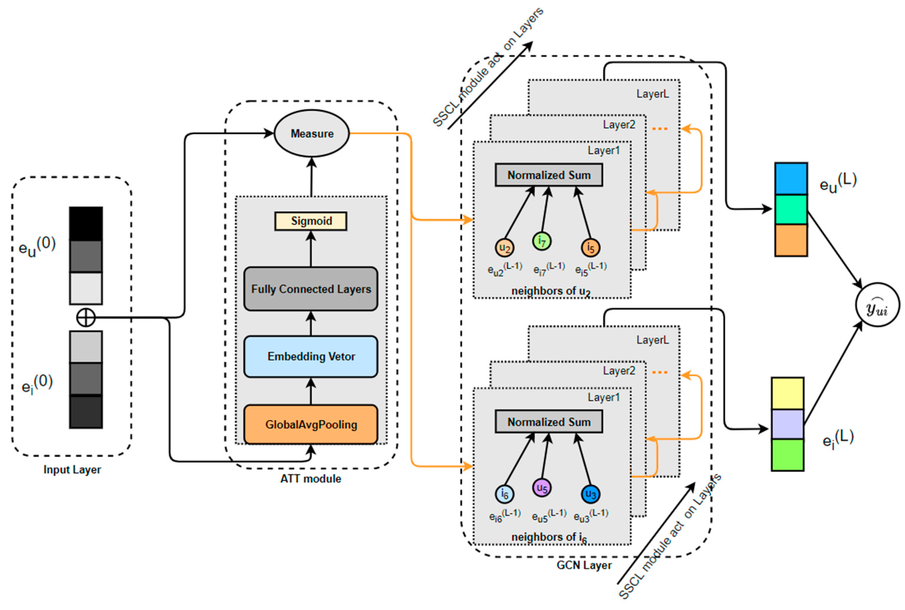
As illustrated in Figure 3, user embeddings and item embeddings are obtained after processing the user–item bipartite graph. These embeddings are then combined and fed into a weight calculation layer. The design concept of this layer is derived from SENet and is composed of global pooling and fully connected layers. The embedding matrix is pooled into a real-valued vector, which is then processed using the attention mechanism from the fully connected layer of SENet to learn this set of real numbers. Ultimately, a set of dimension-invariant attention scores is obtained and multiplied by the original embedding vector, resulting in a weighted new embedding vector. Thus, we refer to this layer as the weight calculation layer. The approach involves suppressing noise or ineffective low-frequency features through the assignment of small weights while amplifying the influence of important features by assigning larger weights. Subsequently, a higher-order aggregation operation is performed on the updated embedding information, enabling the nodes to incorporate information from multi-hop neighboring nodes.

In the next phase, we employ the widely used the LightGCN method for node aggregation, supplemented by a lightweight contrastive learning module to enhance model training. This approach allows us to retain both user and item embeddings while differentiating the importance of various nodes, ultimately aiming to achieve improved prediction scores. We will now provide a detailed explanation of our methodology.

4.2. Input Layer

Early recommendation systems typically utilized a one-hot encoded matrix representing user–item interactions. However, the high sparsity of this matrix posed significant challenges. The advent of matrix factorization techniques alleviated this issue by innovatively approximating the original interaction matrix with the product of user and item embedding matrices, thereby greatly reducing input data redundancy. Consequently, embedding matrices have become the foundational input layer for subsequent research in recommendation systems.

In this paper, we adopt a commonly used embedding layer as the input, which addresses the inefficiency of resource utilization associated with one-hot encoding and facilitates dimensionality reduction, thereby enhancing computational efficiency. We define the input layer of asGCL as follows:

$$E=\left[e_{u_1},\dots ,e_{u_M},e_{i_1},\dots ,e_{i_N}\right],$$

(6)

where $M$ and $N$ represent the number of user and item embedding vectors, respectively. $e_u\in {ℝ}^D$ denotes the user embedding, while $e_i\in {ℝ}^D$ represents the item embedding. Subsequently, the user embeddings and item embeddings are concatenated and fed into the next layer.

4.3. Att Module

The ATT module refers to the attention mechanism module, which consists of two components: dimensionality reduction and fully connected layers. It can also be understood as a weight calculation layer, as we employ the attention mechanism to assign weights to the reduced embedding vectors.

4.3.1. Reduction

Feature fusion is a crucial method in the field of pattern recognition. In the domain of computer vision, image recognition, as a specific pattern classification problem, continues to face numerous challenges. Feature fusion techniques can synergistically leverage multiple image features, achieving complementary advantages and yielding more robust and accurate recognition results. Deep Matrix Factorization (DeepFM) [5] addresses the cold start problem by utilizing a wide and deep network to capture interactions between latent features. The core idea of the Deep Interest Network (DIN) [7] is to incorporate the attention mechanism into user interest modeling. This approach introduces the concept of weights for the pooling of traditional multi-valued features, with the weights determined by the relevance of item features.

The plug-and-play characteristics of SENet and MS_CAM methods have drawn our attention, as both utilize global pooling to transform images from three dimensions to one dimension. Practical applications in the recommendation domain indicate that the mean effect tends to outperform the maximum effect. This is easily understandable; in the visual domain, the strongest features among the convolutional kernel elements are required, whereas in the recommendation domain, averaging better preserves information. Consequently, we apply global average pooling to the embeddings.

Firstly, the embeddings are input into the ATT module with a shape of $\left[N,D\right]$, and then they are naturally reduced in dimensionality to $\left[N,1\right]$ through global average pooling. We represent the data flow of this module using the following formula:

$$at{t}_0=E=\left[e_u\oplus e_i\right],$$

(7)

$$at{t}_1=Global\_avg\_pooling\left(at{t}_0\right).$$

(8)

where ⊕ denotes the concatenation of two embedding matrices.

4.3.2. Fully Connected Layers

The fully connected layer is a component of the ATT module, serving as the weight calculation layer. It processes the reduced embedding vectors obtained in the previous section and assigns weight values to the nodes in the embedding matrix by learning the feature information contained within the vectors.

After pooling, it is essential to learn higher-order feature fusion capabilities; therefore, we introduce a multi-layer neural network. The primary function of the first layer is to perform feature crossing, while the final layer is responsible for maintaining the output dimensionality. Assuming that the embedding layer consists of m features, we must ensure that m weight values are outputted, with the $i_{th}$ weight value corresponding to the $i_{th}$ node embedding. By combining the learned weight information from the fully connected layer with the original node embeddings, we can compute a new node embedding that incorporates these weights.

The reduced embedding vectors serve as the input to the fully connected layer, and the weights and biases of each fully connected layer are initialized randomly according to a Gaussian distribution. The final output is the accumulated result of multiple layers. The weight information of the nodes is derived from the learning of the nonlinear layers. Ultimately, the fully connected layer does not alter the dimensions of the original embedding matrix, which remains as [N,D].

The mathematical expression for the fully connected layer is as follows:

$$\mathrm{s}=\mathrm{F}\left(at{t}_1,\mathrm{W}\right)=\sigma \left(g\left(at{t}_1,\mathrm{W}\right)\right)=\sigma \left({\mathrm{W}}_2\delta \left({\mathrm{W}}_{1}at{t}_1\right)\right),$$

(9)

$$at{t}_2=\mathrm{s}\otimes at{t}_1.$$

(10)

where $\mathrm{s}$ represents a one-dimensional vector that serves as the core of this module, specifically the feature weights. $\mathrm{W}$ represents the weight matrix of the fully connected layer. $\delta$ and $\sigma$ denote the activation functions, and ⊗ denotes that each element in the vector $\mathrm{s}$ is multiplied by each row in the matrix $at{t}_0$, respectively.

Additionally, we introduce an adjustable parameter mc, which represents the number of fully connected layers. To investigate the impact of this parameter on model performance, we conduct ablation experiments in the subsequent experimental section.

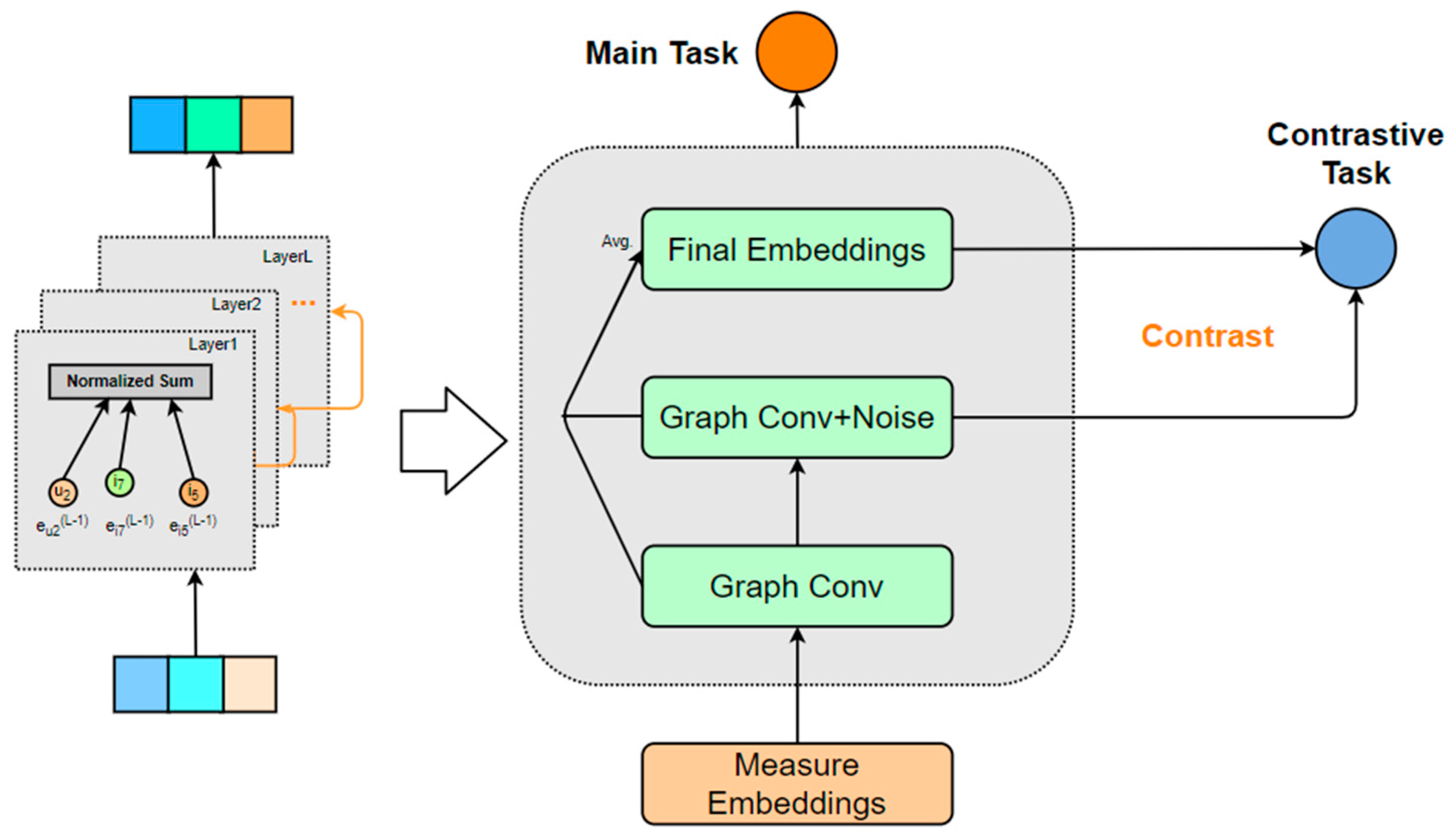
4.4. SSCL Module

Contrastive learning has recently revitalized the field of recommendation systems. Typically, recommendation approaches based on contrastive learning can be divided into two steps. The first step involves introducing structural perturbations to the original user–item bipartite graph, and the second step focuses on maximizing the representations learned from the different perturbed graphs. This paradigm has proven to be effective.

However, recent studies have confirmed that structural perturbations of the bipartite graph are not essential; rather, the critical factor lies in representation learning. Additionally, the choice of the contrastive loss function is also a significant factor, as it can facilitate a more uniform distribution of user–item representations and mitigate certain popularity biases. Consequently, we propose to introduce a graph-augmentation-free contrastive learning method into the model while ensuring that it retains lightweight characteristics. By adding uniform noise between different layers of graph convolution and contrasting the representations across these layers, we achieve a lightweight model akin to LightGCN, thereby realizing a single-channel integration of graph convolution and contrastive learning, which simplifies the computational process. The overall architecture of the module is illustrated in Figure 4.

To address the contrastive learning task, we need to improve the overall design of the model’s loss function [29]. Since we have eliminated graph augmentation and adopted inter-layer comparisons to compute the contrastive loss, our loss function can be expressed as follows:

$$L=L_{rec}+\lambda L_{sscl},$$

(11)

$$L_{sscl}={{\displaystyle \sum }}_{i\in \mathcal{B}}-\log {\displaystyle \frac{\exp \left(z_i^{\prime \top }{z}_i/\tau \right)}{{{\displaystyle \sum }}_{j\in \mathcal{B}}\exp \left(z_i^{\prime \top }{z}_i/\tau \right)}}.$$

(12)

where $L_{rec}$ represents the BPR loss [30] for the primary task, $L_{sscl}$ denotes the loss for the contrastive learning task, $z^{\prime }$ refers to the learned embedding representations from different convolutional layers, and $\lambda$ is a hyperparameter that indicates the strength of the contrastive task.

4.5. Prediction Layer

The prediction layer primarily focuses on the weighted user and item embeddings, as contrastive learning can be regarded as an independent task. We adopt the message-passing framework from LightGCN, maintaining the same depth of three layers to obtain the final results as previously described

$$e_u={{\displaystyle \sum }}_{k=0}^K{\alpha }_k{e}_u^k, e_i={{\displaystyle \sum }}_{k=0}^K{\alpha }_k{e}_i^k.$$

(13)

Finally, the new item scores are calculated using the final embeddings returned by the model to predict each user’s preferences for items they have not yet seen. The scoring function is represented as the scalar product of the embeddings, which can be efficiently computed through matrix multiplication and is expressed as follows:

$${\widehat{y}}_{ui}=e_u^T{e}_i.$$

(14)

5. Experiments

In this section, we conduct a detailed experimental study of the asGCL model. In Section 4.1, we provide a brief introduction to the four real-world datasets utilized in the experiments. In Section 4.2, to better validate the performance of the asGCL model, we place it within the context of these datasets and compare it against several state-of-the-art models. In Section 4.3, we explore the roles of various modules within the model and examine the impact of adjusting certain hyperparameters on its performance.

5.1. Datasets

Table 1. Statistics of datasets.

Dataset	#User	#Item	#Interact	Sparsity
M1-1M	6039	3628	836,477	96.18%
Gowalla	29,857	40,979	1,027,464	99.93%
Yelp2018	31,608	38,044	1,561,386	99.86%
Amazon-Books	35,737	38,522	2,060,674	99.85%

contains four statistics, where #User indicates the number of users, #Item indicates the number of items, #Interact indicates the number of interactions between users and items, and Sparsity represents the sparsity of the interaction matrix, which is the proportion of zero elements in the matrix.

The datasets are available at https://github.com/CyberAres/Datasets (accessed on 28 February 2025). We conduct experiments on widely used public datasets as follows:

• Gowalla [31] is an important resource for studying social networks, user behavior, and location-based services. It encompasses GPS trajectories, social friendship relations, and location activity classifications. This resource is widely utilized in the fields of social computing, geographic information science, and recommendation systems.
• Amazon-Books [32]. It is a large-scale book review dataset provided by Amazon containing information on book reviews from the years 2000 to 2019.
• Yelp2018 [33]. Based on real feedback and interactions on the platform, it includes a large number of reviews and ratings from various business scenarios across multiple cities. It can reflect user consumption habits and market trends.
• Movielens-1M [34]. It comprises a substantial amount of user ratings for a wide array of films, playing a crucial role in personalized recommendation systems and social psychology. The statistical information of the dataset is presented in the table below. Each interaction is considered a positive instance, and a negative pairing is extracted for each user.

5.2. Metrics and Baselines

5.2.1. Metrics

We employed a popular full-ranking strategy for candidate items that have not interacted with all users, utilizing widely adopted collaborative filtering performance evaluation metrics in the recommendation domain: recall@K and NDCG@K, with K set to 20. Higher values of these two metrics indicate better performance. The top K recommendation is a common task in recommendation systems and is aimed at suggesting the top K most relevant items to users. Therefore, K in recall@K and NDCG@K also represents this meaning.

• recall@K. It is defined as the proportion of correctly predicted relevant results among all relevant results, which can be expressed as follows:

  $$recall@K={\displaystyle \frac{TP@K}{TP@K+FN@K}}.$$

  (15)

  where $TP$s (True Positives) refer to the samples that are truly positive and are also predicted as positive, while $FN$s (False Negatives) refer to the samples that are truly positive but are predicted as negative.
• NDCG@K. Normalized Discounted Cumulative Gain (NDCG@K) is defined as follows:

  $$NDCG@K={\displaystyle \frac{DCG@K}{IDCG@K}}.$$

  (16)

  where $DCG$ (Discounted Cumulative Gain) represents the cumulative score of the relevance values of each recommended item, taking into account the positional impact of the recommendations within the list. $IDCG$ (Ideal Discounted Cumulative Gain) is assumed to be the $DCG$ value of the optimal recommended list returned for a specific user.

5.2.2. Baselines

We compare asGCL with popular baselines and describe them briefly as follows:

• BPRMF [3]. This is a fundamental matrix factorization algorithm, and the objective of BPR (Bayesian Personalized Ranking) is to maximize the score difference between items that have been interacted with and those that have not. In straightforward terms, it aims for the items that users have accessed to receive higher ratings. This algorithm has become a foundational concept in the subsequent development of recommendation systems.
• NeuMF [4]. This algorithm specializes in matrix factorization and extends it to Generalized Matrix Factorization (GMF). Building upon this foundation, it explores deep learning by employing a multi-layer perceptron to learn the interaction function between users and items. This approach integrates the linear advantages of matrix factorization with the nonlinear benefits of multi-layer perceptrons.
• GCMC [35]. The link prediction problem can be framed as a matrix completion task. The Graph Convolutional Matrix Completion (GCMC) method designs a differentiable message-passing-based graph autoencoder framework that generates latent features within a bipartite interaction graph. This approach effectively integrates interaction data with edge information.
• GAT [36]. The model computes the corresponding latent information for each node and incorporates a single-layer feedforward neural network into the graph structure through masked attention. This mechanism focuses solely on calculating the first-order neighboring nodes of the target node.
• NGCF [6]. It uncovers collaborative signals in the interactions between users and items, integrating these signals into the embedding process. The model introduces encoding methods for node message construction and message aggregation, whereby stacking multiple message aggregation layers enables the extraction of higher-level collaborative information.
• LightGCN [13]. It is an embedding-based model that inherits and enhances the principles of NGCF (Neural Graph Collaborative Filtering). By eliminating the complex design of multi-layer nonlinear feature transformations, it employs a simple weighted sum aggregator to effectively capture the effects of graph convolution and self-connections. This lightweight and efficient approach has made it quite popular.
• SGL [19]. It generates multiple views of the same node through data augmentation, maximizing the similarity between different views while minimizing the similarity between representations of different nodes. This approach aids in uncovering challenging negative sample information, leading to improved recommendation performance, particularly for long-tail items.
• LightGCL [21]. LightGCL posits that heuristic-based augmentation techniques for generating contrastive views do not effectively preserve the intrinsic semantic structure. Consequently, it specifically employs singular value decomposition for contrastive enhancement, thereby modeling collaborative relationships more effectively.

5.3. Implement Details

The experimental hardware platform we employed is a 24GB RTX 4090 GPU, and all models discussed in this paper are implemented using the PyTorch 1.7.1 framework. The batch size for the training dataset is set to 4096. In terms of the embedding layer and the weight computation layer, the embedding size is set to 64 for all methods based on embedding, and the learning rate is set to 0.001. The fully connected layer was activated by relu. The number of layers for all models based on convolutional layer node aggregation is set to 3.

5.4. Overall Performance

In this section, we conduct a comprehensive performance comparison of asGCL against various baselines across four datasets. Additionally, we retrain asGCL and the best-performing baseline five times to compute p-values. The results are presented in

Table 2. Performance comparison of the baseline with our model. The best result values are indicated in bold.

Dataset	Metrics	BPRMF	NeuMF	GCMC	GAT	NGCF	LightGCN	SGL	LightGCL	asGCL	p-Val.	Improv.
Amazon-Book	R@20	0.0764	0.0575	0.0711	0.0729	0.0760	0.0954	0.1002	0.1021	0.1064	$1.4\times e^{-2}$	4.21%
	N@20	0.0474	0.0345	0.0557	0.0574	0.0472	0.0614	0.0659	0.0675	0.0734	$1.0\times e^{-3}$	8.74%
Gowalla	R@20	0.1686	0.1470	0.1485	0.1523	0.1633	0.1882	0.2109	0.2112	0.2197	$5.3\times e^{-4}$	4.02%
	N@20	0.0965	0.0808	0.0812	0.0857	0.0937	0.1099	0.1134	0.1133	0.1203	$1.1\times e^{-6}$	6.11%
Yelp2018	R@20	0.0764	0.0548	0.0915	0.0939	0.0778	0.0914	0.0947	0.0889	0.0990	$3.0\times e^{-3}$	4.63%
	N@20	0.0460	0.0316	0.0488	0.0513	0.0472	0.0567	0.0588	0.0592	0.0614	$2.3\times e^{-2}$	3.71%
ML-1M	R@20	0.2637	0.2455	0.2611	0.2656	0.2695	0.2647	0.2697	0.2717	0.2872	$5.3\times e^{-6}$	5.70%
	N@20	0.2464	0.2267	0.2464	0.2473	0.2483	0.2511	0.2553	0.2530	0.2667	$1.4\times e^{-2}$	4.47%

.

We can draw the following experimental conclusions:

• We propose that asGCL consistently outperforms all baseline models across various datasets and metrics. Specifically, asGCL achieves relative improvements of 19.5% and 9.46% over LightGCN on the Amazon-Books and Gowalla datasets, respectively, in terms of NDCG@20. On the Yelp2018 and ML-1M datasets, asGCL shows relative enhancements of 8.31% and 8.50% over LightGCN in Recall@20. Compared to the strongest baseline model, LightGCL, asGCL also demonstrates superior performance, with Recall@20 improvements of 4.21%, 4.02%, 11.36%, and 5.70% and NDCG@20 improvements of 8.74%, 6.17%, 3.71%, and 5.41% across the same datasets. Furthermore, models based on graph convolution networks generally outperform those based on matrix factorization, as evidenced by LightGCN’s significant advantage over previous baselines. Additionally, graph contrastive learning methods, such as SGL and LightGCL, exhibit performance gains over LightGCN across all four datasets.
• Represented by LightGCN and BPR, GNN-based methods outperform matrix factorization methods, indicating the positive role of higher-order node information in the learning process. As noted, asGCL demonstrates the best performance across all four datasets. Specifically, on the Amazon-Books dataset, asGCL achieves improvements of 4.21% in recall@20 and 8.74% in NDCG@20, which clearly indicates a significant advancement in our model’s performance. The incorporation of weight information for nodes along with contrastive learning methods in asGCL represents an effective research direction. Summarizing the impressive results exhibited by our model, we attribute this performance to the following factors. (1) The lightweight attention mechanism of asGCL further amplifies the differences among nodes. (2) Compared to other baseline models, the contrastive learning method introduced by asGCL indeed brings considerable performance improvements. This approach contrasts across layers with uniform noise and is more inclined towards representation learning rather than graph enhancement, as we believe that uniform node distribution and the contrastive loss function are crucial factors contributing to the effectiveness of contrastive learning.
• Compared to GCN, collaborative filtering methods that employ contrastive learning models demonstrate significant performance improvements across nearly all metrics. The contrastive information embedded in the contrastive learning approach (specifically, the contrastive loss function) contributes substantially to the enhanced generalization ability of collaborative filtering. This improvement is primarily attributable to the theoretical shortcomings of the BPR (Bayesian Personalized Ranking) pairwise relative ranking loss, which introduces a large number of ineffective negative samples during the training process. Additionally, BPR typically assumes that unlabeled data are all negative samples, which adversely affects the model’s performance.
• In general, graph convolutional network (GCN) models outperform traditional web embedding models; however, the performance of these models is contingent upon the volume of data. As evidenced by the table, GCNs exhibit significantly better performance on the Gowalla and Yelp2018 datasets, whereas their advantage on the Movielens-1M dataset is less pronounced. GCNs excel at uncovering higher-order collaborative information, making them more suitable for complex and large datasets. Conversely, for simpler and sparser datasets, lightweight models tend to achieve better results more readily.

5.5. Further Study

In this section, we conduct a more detailed exploration of the various modules of asGCL and design several ablation experiments to validate the model’s effectiveness and robustness.

• The impact of the number of fully connected layers on model performance is explored, with numerical settings of $\left[1,2,3\right]$.
• We conduct an analysis of the ablation experiment results for the weight calculation module and the contrastive learning module.
• We perform comparative experiments with different data augmentation methods to evaluate their effects.
• The SSCL module includes a hyperparameter $\lambda$, which represents the strength of the contrastive learning task.

5.5.1. Effect of $\mathrm{mc}$

The parameter $mc$ represents the number of fully connected layers in the attention module applied to the reduced embedding. This parameter reflects the strength of the original input information and the model’s capacity for function fitting. Our goal in using this parameter is to identify an optimal value that maximizes model performance.

In this set of experiments, we set $mc$ to range from 1 to 3. When $mc=1$, the data pass through a single fully connected layer that is represented mathematically as

$$\mathrm{F}\left(at{t}_1,\mathrm{W}\right)=\sigma \left({\mathrm{W}}_{1}at{t}_1\right).$$

(17)

Similarly, when $mc=2$, the expression becomes

$$\mathrm{F}\left(at{t}_1,\mathrm{W}\right)=\sigma \left({\mathrm{W}}_2\delta \left({\mathrm{W}}_{1}at{t}_1\right)\right),$$

(18)

where $at{t}_1$ denotes the pooled embedding vector in the attention module and $\delta$ and $\sigma$ represent activation functions, with the final layer’s activation function always being $\sigma$. In Figure 5, we can observe the following:

• Figure 5a shows that on the m1-1m dataset, both recall@20 and ndcg@20 exhibit lower values when $mc=1$, a significant improvement at $mc=2$, and a slight decline at $mc=3$. In the Gowalla dataset shown in Figure 5b, recall@20 demonstrates a clear performance trend, while the difference in NDCG@20 between $mc=1$ and $mc=2$ is less pronounced; both metrics display a trend of initial increase followed by a decrease. It is evident that a greater number of fully connected layers results in a higher training burden on the model. The experimental results are optimal when the number of layers is set to 2. Although this configuration incurs a higher training cost, it is acceptable in light of the performance enhancement it provides.
• When the number of layers exceeds 2, the experimental results decline rather than improve, and the training consumption continues to rise. Therefore, it is clear that further increasing the number of layers does not yield any benefits for the model.

5.5.2. Ablation of the Module

In this section, we will examine the performance of two variants of asGCL to validate the effectiveness of the various modules within the model. The different variant configurations are as follows: (1) the removal of the node weight computation module, utilizing only the contrastive learning module, denoted as asGCLs; (2) the removal of the contrastive learning module, utilizing only the node weight computation module, denoted as asGCLa. The experimental results are presented in the table. In Figure 6, we observe that both enhancement components employed in the model contribute to some performance improvement without any degradation. Moreover, compared to the contrastive learning module, the node weight computation module provides a slightly greater performance enhancement to the model.

5.5.3. Data Augmentation

The attention module in asGCL can be regarded as a form of data augmentation. To explore the true capabilities of this method more deeply, we selected two negative sampling strategies for comparison with our model based on LightGCN. Random Negative Sampling (RNS) can be described as a process that involves removing items that have interacted with the target user from the entire sample set and then randomly selecting from the remaining items as negative samples. In contrast, Dynamic Negative Sampling (DNS) [37] is a model-based algorithm that adjusts the sampling probability of negative samples based on the scores generated from the previous round of model training.

The experimental results in

Table 3. Performance comparison of different data augmentation strategies.

Dataset	Metrics	LightGCNrns	LightGCNdns	asGCLa
Amazon-Books	R@20	0.0973	0.1008	0.1039
	N@20	0.0638	0.0674	0.0695
Yelp2018	R@20	0.0931	0.0945	0.0979
	N@20	0.0567	0.0589	0.0614

indicate that our method still demonstrates a certain degree of superiority.

5.5.4. Hyperparameter of the SSCL Module

In the contrastive learning module, $\lambda$ represents the task intensity. We conducted experiments on the Amazon-Books dataset using various $\lambda$ values within the range of [0.01, 0.05, 0.1, 0.2, 0.5, 1]. As illustrated in Figure 7, with the gradual increase in $\lambda$, both recall@20 and NDCG@20 metrics exhibit an upward trend, indicating that the contrastive learning task indeed contributes to the enhancement of model performance. When $\lambda$ is in the range of [0.05, 0.1, 0.2], the model demonstrates relatively high and stable performance on the dataset. Notably, when $\lambda$ = 0.2, both metrics reach their peak values, signifying that an appropriate weight of contrastive loss in the overall loss calculation can effectively balance the main and auxiliary tasks, thereby improving model performance. However, as $\lambda$ continues to increase, both metrics experience a decline, particularly when $\lambda$ = 1, where a significant drop in performance is observed. This may suggest that an excessively high task intensity for the contrastive task adversely affects the performance of the primary recommendation task. Overall, it is essential to maintain $\lambda$ within a moderate range; setting it too low may fail to leverage the node distribution capabilities brought by the contrastive task, while setting it too high could suppress the primary recommendation task and degrade the quality of the embedding representations from the preceding layers. Therefore, we recommend setting $\lambda$ around 0.2 to ensure a balance between the main and auxiliary tasks, aiming for optimal model performance.

5.5.5. Efficiency of the Model

We designed a series of experiments to evaluate the training efficiency of asGCL. We selected two representative models to compare training time and epochs. The LightGCN model features a streamlined architecture and strong interpretability, while LightGCL serves as a paradigm for contrastive learning. As shown in

Table 4. Training comparison of different models on Yelp2018.

Model	Time/Epoch	Epoch	Training Time
LightGCN	85.33 s	293	7.1 h
LightGCL	89.06 s	264	6.5 h
asGCL	92.12 s	235	6.2 h

, LightGCN has the shortest training time per epoch at 85.33 s, but it requires more epochs. In contrast, asGCL has a longer training time per epoch, but it requires fewer epochs at 235, resulting in a reduced total training duration. Thus, our model demonstrates a certain advantage in training time efficiency.

6. Conclusions and Future Work

This paper explores and reflects on graph collaborative filtering recommendation systems, providing a profound analysis of the data representation of embedding-based models. Inspired by the application of channel attention mechanisms in the field of computer vision, we propose the asGCL model, which simulates the attention mechanism to compute node weight scores on the embedding matrix. Additionally, we incorporate a single-channel contrastive learning approach; through this data augmentation technique, our model achieves performance improvements across four classical datasets. Furthermore, our model is highly flexible and modular, allowing for easy disassembly. Our work enhances the data augmentation methods in graph collaborative filtering to a certain extent.

Based on our experiments, our model demonstrates significant performance improvements compared to traditional matrix factorization-based recommendation systems, such as BPRMF, as well as graph convolutional network-based systems, like LightGCN and SGL. This is particularly evident in the Amazon-Books dataset, indicating that the combination of attention mechanisms and contrastive learning has substantial application value in the recommendation system domain.

In our ablation studies, we found that the fully connected layers in the ATT module are best configured with two layers, as this choice preserves the nonlinearity between node features without excessively burdening model training. We then compared the contributions of the ATT module and the SSCL module within the overall model. Our findings indicate that the ATT module provides a slightly greater performance boost than the SSCL module when used independently, although the SSCL module also demonstrates a positive effect.

Furthermore, we explored the advantages of using the ATT module alone against state-of-the-art (SOTA) approaches. The results are encouraging, as we maintain a lead over the strategy-enhanced LightGCN. Finally, we conducted a separate study on the SSCL module and discovered that the strength of contrastive learning as an auxiliary task is crucial for model performance. Specifically, setting the value of $\lambda$ to 0.2 allows this module to achieve peak performance.

In future research, we will continue to explore the potential integration of advanced attention mechanisms with graph convolutional networks and investigate new directions in graph contrastive learning. Our objective is to enhance the capability of recommendation systems to mitigate popularity bias and elevate the development and applicability of graph convolutional recommendation systems to new heights.