Case Study on Analysis of Soil Compression Index Prediction Performance Using Linear and Regularized Linear Machine Learning Models (In Korea)

Abstract

The compression index (C_c) is a critical soil parameter that is used to estimate the consolidation settlement of ground. In this study, the compression index, typically obtained through consolidation tests, was predicted using machine learning techniques after preprocessing data that considered the geotechnical and hydrogeological characteristics of the study area. This approach enabled an analysis of how geotechnical and hydrogeological characteristics affect the performance of machine learning models. Data obtained from geotechnical investigations were used to train models for each classified zone. Suitable models were then selected to predict the compression index, and their performance was evaluated. Predictions that considered the geotechnical and hydrogeological characteristics showed improved accuracy in zones influenced by a single water system or zones near the coast. However, in offshore areas with complex water systems, using the entire dataset proved to be more effective. Differences in the clay mineral of the soil also affected the prediction accuracy, indicating a correlation between clay mineral properties and model performance. These findings suggest that classifying data based on geotechnical and hydrogeological characteristics is necessary when developing compression index prediction models to achieve relatively stable results.

1. Introduction

Demand for land development to support infrastructure continues to rise. Given this, the improvement and reclamation of soft ground has been actively undertaken across the globe including in the coastal areas of South Korea [1,2,3]. Soft ground refers to soil with low shear strength and high compressibility [4], where clay and silt make up a significant portion. The behavior of silts and clays is dependent on the applied loading conditions, making it difficult to predict their behavior [5]. This is particularly the case with clay. The microstructure and swelling potential of clay can vary significantly depending on the soil’s water content and the type and proportion of clay minerals it contains [6,7]. This variation challenges our understanding of the behavior of soft ground, increasing the likelihood of failures and ultimately causing extensive damage to infrastructure [8]. Factors, such as the inaccurate determination of design parameters during soft ground improvement, frequently give rise to soil consolidation and differential settlement, which in turn lead to structural failures [9]. Therefore, a precise estimation of consolidation settlement is essential, if the structural safety and sustainability of structures built on soft ground is to be assured [10].

To accurately predict consolidation settlement, the consolidation characteristics of the soil must be carefully considered during the construction phase. This makes a precise determination of the compression index of vital importance. The compression index (C_c), defined as the slope of the linear portion of the void ratio–pressure curve obtained from consolidation tests, is a critical soil parameter for estimating the primary consolidation settlement of soft ground. Clay with a high compression index undergoes a greater reduction in void ratio under the same stress change compared with clay with a low compression index. This greater reduction results in larger consolidation settlement. Consequently, the compression index plays a crucial role in understanding the consolidation characteristics of soft ground. However, consolidation tests conducted to determine the compression index are beset with several challenges. These include difficulties in preserving undisturbed soil samples during sampling and transportation, the time-consuming nature of the testing process, and the reliance on the technician’s expertise during the analysis of results [11,12]. Therefore, studies have long been conducted to simplify the estimation of the compression index by utilizing correlations between soil properties and the compression index.

Previously, correlation equations based on linear relationships between single soil parameters, such as natural water content, initial void ratio, liquid limit, and shear wave velocity, and the compression index have been proposed [13,14,15,16,17,18,19,20,21,22]. Moreover, studies have been conducted that not only utilize a single soil parameter, but also identify correlations between multiple geotechnical parameters and the compression index [13,15,16,17,22,23,24,25]. While these traditional empirical equations allowed for a rapid estimation of the approximate compression index values, they had limitations when it came to explaining the complex relationships between the compression index and various independent variables. Consequently, to overcome these limitations, various methods employing machine learning (ML) techniques and soft computing methods that offer solutions to complex real-world problems [26] have been increasingly applied in geotechnical engineering.

Various soft computing and ML techniques, including XGBoost (XGB), artificial neural network (ANN), and genetic algorithm (GA), have been employed for the task of predicting the compression index [16,17,22,27,28,29,30,31,32]. Kalantary and Kordnaeji [17], Kumar and Rani [30], Al-Taie et al. [31], Park and Lee [16], and Majdi et al. [22] predicted the compression index using ANN with a feed-forward back-propagation algorithm. Zhang et al. [32] used GA to optimize the hyperparameters of five models including a back-propagation neural network (BPNN). Mamudur and Kattamuri [27] developed an XGB model to predict the compression index using five geotechnical parameters, while Long et al. [28] and Lee et al. [29] employed XGB along with other models. Additionally, Bardhan et al. [12] optimized the parameters of ANN and adaptive neuro-fuzzy inference system (ANFIS) models by using ten swarm intelligence algorithms. Of these, the ANFIS and PSO hybrid model demonstrated the best performance. Díaz and Spagnoli [33] developed a super-learner machine learning model for compression index prediction. The liquid limit, plasticity index, natural water content, and initial void ratio were used as input values, with the extra trees regressor and gradient boosting regressor algorithms serving as base learners and the random forest regressor algorithm serving as the meta learner. This resulted in a model with a strong predictive performance being developed, achieving a value of R² = 0.93.

Although numerous studies have been conducted to predict geotechnically significant indices using artificial intelligence (AI) techniques, no data preprocessing was carried out prior to training the model. Indeed, even if preprocessing was performed, it was limited to simply removing statistical outliers or performing feature engineering based on computer science approaches. Furthermore, even if a prediction was made, the performance of the model was only analyzed numerically, with the geological elements of the study area not taken into consideration during the prediction and analysis process.

Therefore, this study aimed to analyze the factors influencing variations in the predictive performance of machine learning models by dividing data based on topographical factors in the Saemangeum reclaimed land area, located on the west coast of South Korea. First, geotechnical data comprising five key geotechnical parameters affecting the consolidation of soft ground were extracted from the reports conducted on the study area. The area was then categorized into four zones based on sedimentary characteristics and the water systems. Four ML models, namely multiple linear regression (MLR), ridge regression (RR), lasso regression (LR), and elastic net regression (ENR), were then employed. After optimizing the hyperparameters of each model, prediction of the compression index then took place. The prediction performance of a total of 20 models was evaluated using the model performance metrics R² and root mean squared error (RMSE) for five cases using data from all four zones (1, 2, 3, and 4) as well as the entire Saemangeum data. Finally, the prediction accuracy of the ML models was analyzed in relation to the geotechnical and geological characteristics to verify the reliability of the selected models and methodologies.

2. Overview of the Study Area and Data Validity

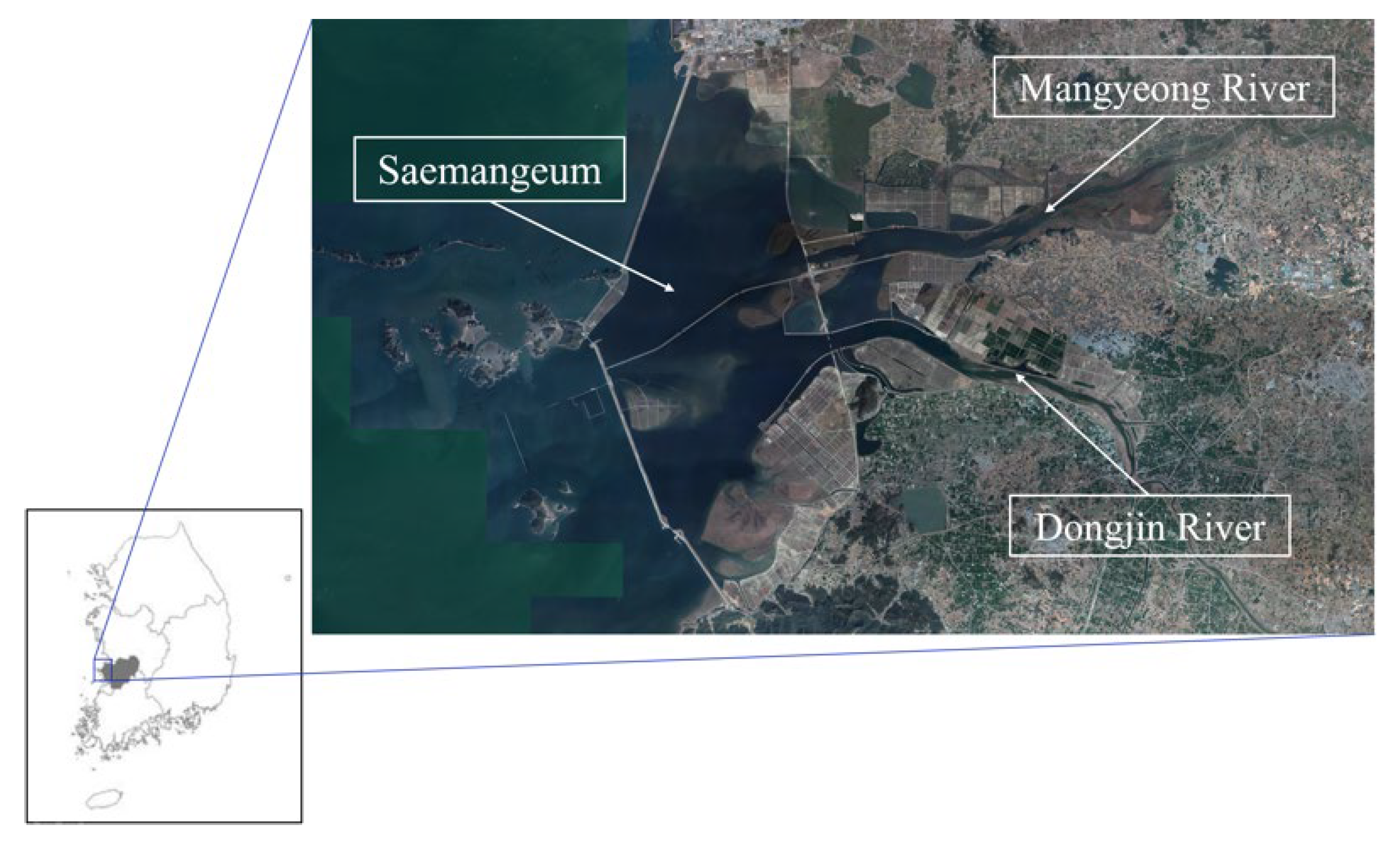
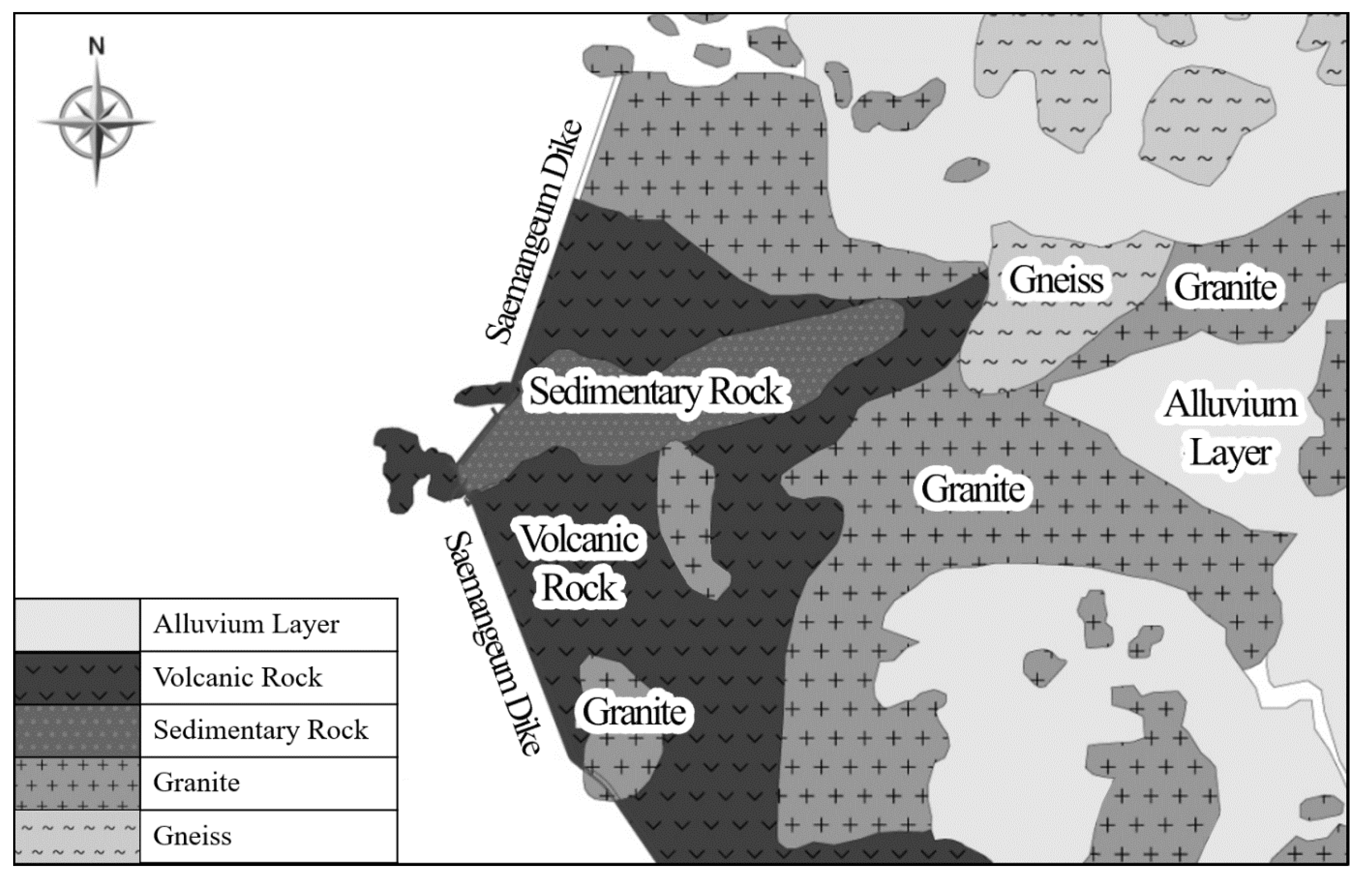
2.1. Hydrogeological Overview of the Saemangeum Reclaimed Land

The Saemangeum reclaimed land area is located adjacent to Gunsan, Gimje, and Buan in Jeollabuk-do, South Korea. It was formed during the course of a large-scale reclamation project involving the construction of a sea dike surrounding the coastlines of these three regions. The project aimed to expand national territory and promote the development of industrial and tourism zones. Saemangeum Lake is supplied by several rivers including seven regional rivers and three small rivers. Of these, two national rivers, the Mangyeong River and the Dongjin River, flow directly into Saemangeum Lake and have the greatest impact. Figure 1 shows a satellite image of the Saemangeum reclaimed land area, showing the Mangyeong River and the Dongjin River flowing into Saemangeum Lake. The topography of Saemangeum has been shaped by the continuous accumulation of sediments transported from the Mangyeong River and Dongjin River over time. Additionally, the construction of the Saemangeum Dike has altered the water flow and sedimentation patterns within the area [34,35,36].

The Mangyeong River flows into the upper part of Saemangeum, while the Dongjin River drains into the West Sea through its lower part. As shown in Figure 2, the lower part of Mangyeong River is underlain by bedrock primarily composed of gneiss and granite, whereas Dongjin River is predominantly underlain by granite bedrock. Consequently, the sedimentary characteristics of the Saemangeum reclaimed land are likely to be influenced by the geological properties derived from the weathering of the bedrock in these two rivers.

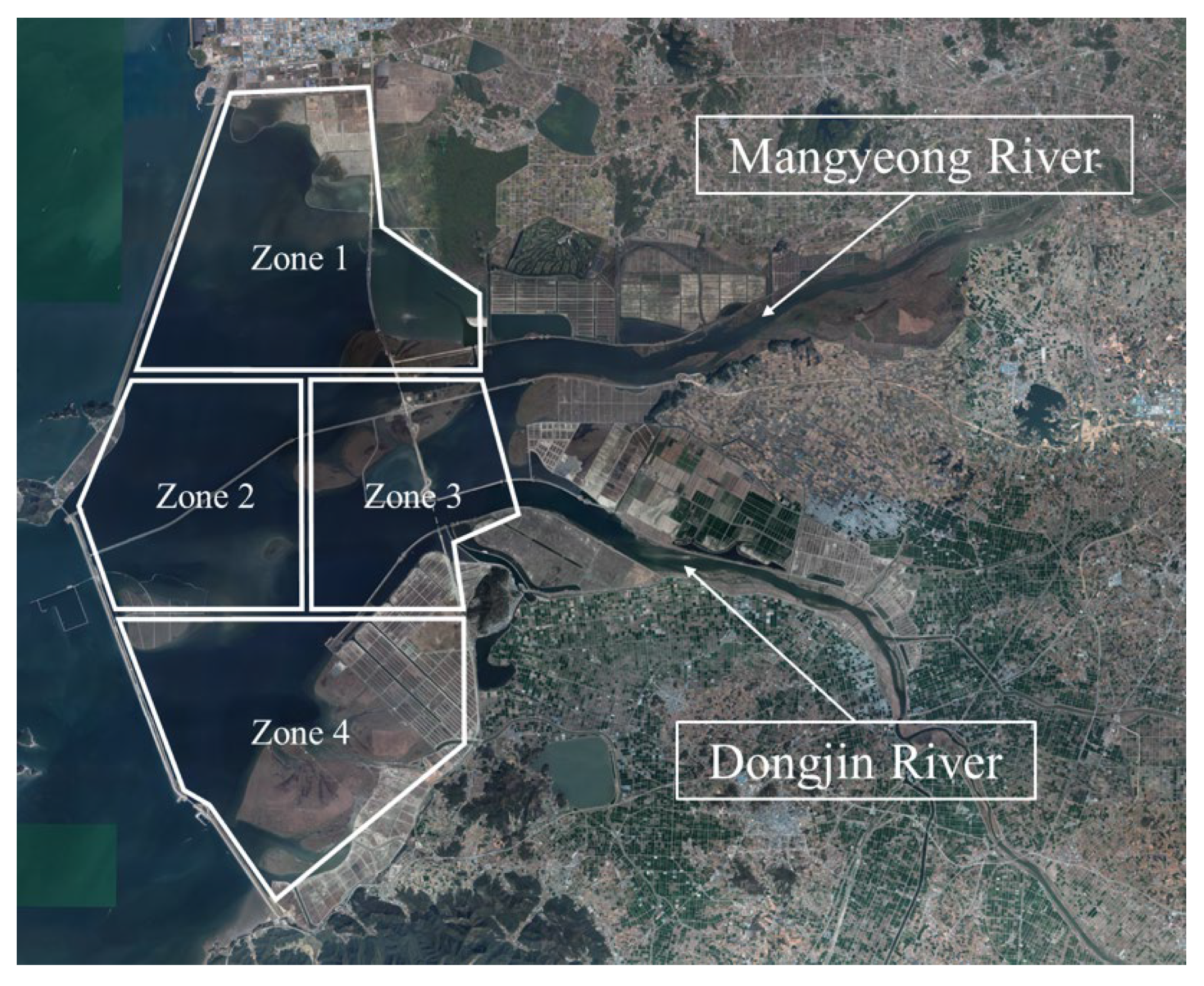
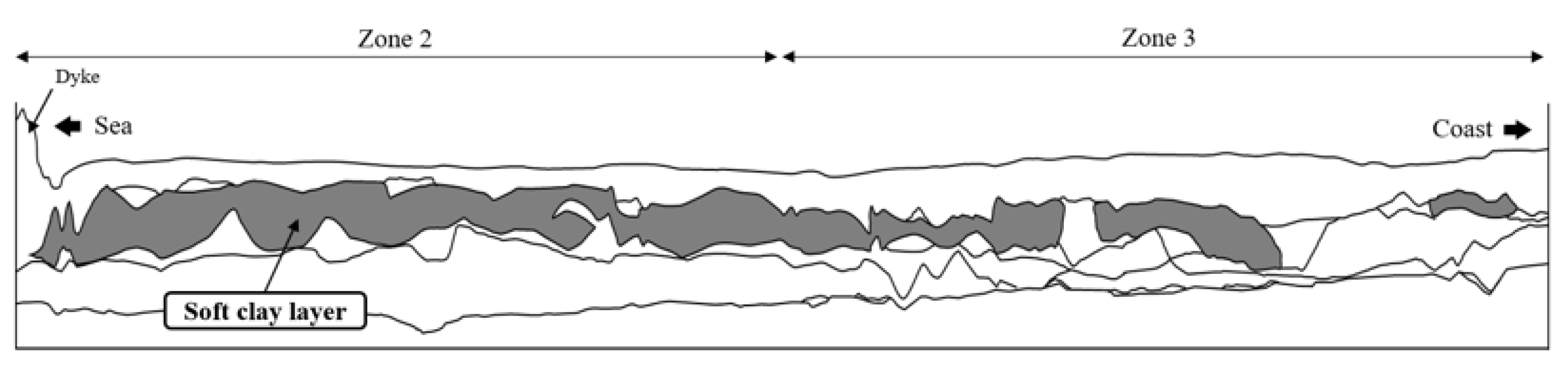
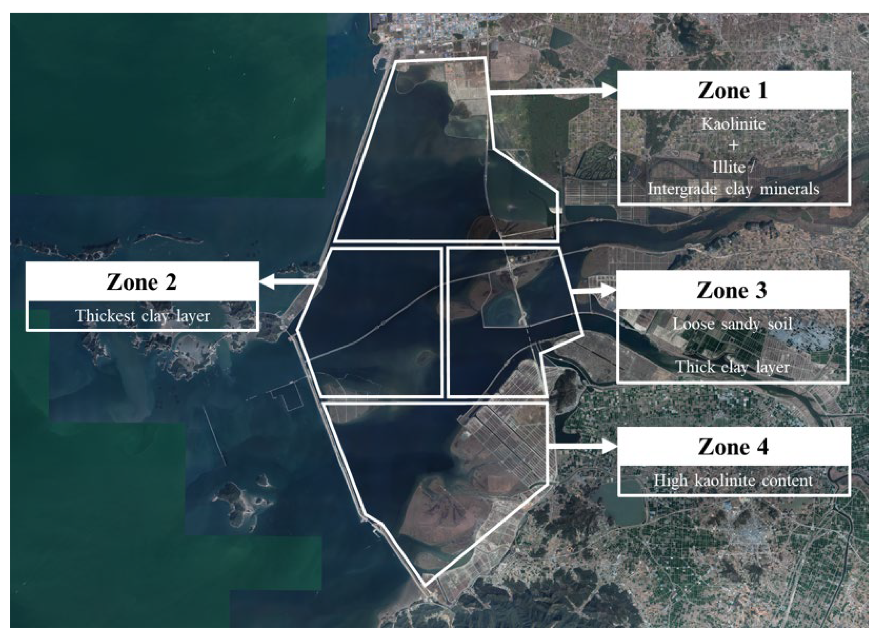
2.2. Zone Classification Based on Water Systems and Geological Characteristics

To investigate the influence of geotechnical and hydrogeological factors on the prediction results of the ML model, the Saemangeum area was divided into four zones based on water systems and geological characteristics. Zone 1 is influenced by the Mangyeong River, while zone 4 is influenced by the Dongjin River. Zone 3 is relatively close to both rivers and is subject to their mutual influence, whereas zone 4 is farther from both rivers but still remains under their mutual impact (Figure 3).

2.3. Data Validation (Assessing the Validity and Reliability of Data)

In this study, the data used were collected from geotechnical investigation reports and final design reports [34,38,39,40,41,42,43,44,45,46,47]. These data were comprised of the findings of geotechnical investigations undertaken for the construction of the east–west road, north–south road, industrial city, and waterfront city in Saemangeum. Considering the variables utilized in empirical equations and machine learning models for predicting the compression index in previous studies, along with various factors influencing the compression index, four geotechnical parameters—natural water content (w_n), liquid limit (LL), plasticity index (PI) and initial void ratio (e₀)—were selected as predictor variables for estimating the compression index (C_c). The validity of these data was evaluated and explained by calculating the Pearson correlation coefficient. The Pearson correlation coefficient is a metric used to describe the linear relationship between variables.

The calculated correlation coefficients between the compression index and the four predictor variables for the given dataset are presented in

Table 1. Pearson correlation coefficients between the C_c and soil properties.

No.	Factor	Correlation Coefficient	p-Value
1	wn	0.7	0.000
2	LL	0.7	0.000
3	PI	0.69	0.000
4	e0	0.75	0.000

. All four variables demonstrated a relatively strong correlation with the compression index [48]. Furthermore, the computed p-values were all below 0.05, confirming their statistical significance as predictors for estimating the compression index.

The geotechnical parameters used in this study were collected from borehole data spanning the entire Saemangeum area. After excluding missing values, a total of 479 datasets were compiled. These datasets were then further divided into zones 1, 2, 3, and 4 based on the hydrogeological characteristics, resulting in 272, 39, 33, and 135 datasets for each zone, respectively. Because the datasets for zone 2 and zone 3 were limited in size, there was a possibility that this constraint may have affected the accuracy of the training and testing outcomes.

Subsequently, statistical analysis was conducted to accurately understand the distribution and range of the collected data (

Table 2. Descriptive statistics of the entire dataset.

		Min	Max	Mean	Std
Input Variable	wn (%)	17.7	68.3	36.379	6.96
	LL (%)	24.9	94	46.482	13.046
	PI (%)	2.2	62.8	24.778	13.295
	e0	0.541	1.88	1.019	0.181
Output Variable	Cc	0.03	0.93	0.359	0.127

). The natural water content exhibited a relatively wide distribution, ranging from 17.7% to 68.3%, while the liquid limit demonstrated substantial variation between 24.9% and 94%. The plasticity index, with a standard deviation of 13.295, exhibited a distribution pattern similar to that of the liquid limit. The initial void ratio ranged from 0.541 to 1.88, indicating low variability, while the compression index, varying between 0.03 and 0.93, exhibited the smallest standard deviation among all geotechnical parameters.

All analyses in this study were performed using Python version 3.11.5, along with the Scikit-learn library. The dataset was split into a training dataset for model training and a testing dataset for performance evaluation, with a ratio of 8:2.

3. Machine Learning Techniques Based on Linear and Regularized Linear Models

3.1. Linear and Regularized Linear Models

3.1.1. Multiple Linear Regression (MLR)

Linear regression is one of the most widely used regression methods, aiming to identify the best-fit line that represents the relationship between the dependent and independent variables. Multiple linear regression, a type of linear regression, models the relationship between multiple independent predictor variables and a single dependent outcome variable. This stands in contrast to simple linear regression, which focuses on the relationship between a single independent variable and a single dependent variable [49]. If the predictor variables are denoted as $x_1$ to $x_n$ and the outcome variable as $y$, the relationship between $x$ and $y$ can be expressed as shown in Equation (1):

$$y={\beta }_0+{\beta }_1{x}_1+{\beta }_2{x}_2+\cdots +{\beta }_n{x}_n+\epsilon$$

(1)

where ${\beta }_0$ denotes the intercept, ${\beta }_1$ to ${\beta }_n$ denote the weights, and $\epsilon$ denotes the error term. The intercept and weights together are referred to as regression coefficients. The weights of the regression equation were calculated using the ordinary least squares (OLS) method, which minimizes the residual sum of squares (RSS), defined as the sum of the squared differences between the observed data points and the values predicted by the regression equation [29,50]. For a training dataset consisting of m samples, the cost function for linear regression was defined as shown in Equation (2). The primary goal of linear regression is to identify the regression coefficients that minimize this cost function.

$${MLR}_{cost}=\sum _{i=1}^m{(y_i-\widehat{y_i})}^2$$

(2)

Here, $y_i$ represents the actual value of the i-th training data, while $\widehat{y_i}$ denotes the predicted value of the i-th training data.

3.1.2. Ridge Regression (RR)

Ridge regression, also known as Tikhonov regularization, is a model designed to address the limitation of linear regression, where regression coefficients can become excessively large. It does so by adding an L2 regularization term to linear regression, ensuring that the model weights remain small. The cost function of ridge regression incorporates the L2 regularization term $\lambda \sum _{j=1}^n{\beta }_j^2$, in addition to the cost function of linear regression. This regularization term helps reduce the weights during the training process [51,52,53]. The cost function of ridge regression is presented in Equation (3):

$${RR}_{cost}=\sum _{i=1}^m{(y_i-\widehat{y_i})}^2+\lambda \sum _{j=1}^n{\beta }_j^2={MLR}_{cost}+\lambda \sum _{j=1}^n{\beta }_j^2$$

(3)

where $\lambda$ is the regularization parameter, controlled by the hyperparameter alpha. As $\lambda$ increases, the regularization strength becomes greater, and the model’s weights decrease [54].

3.1.3. LASSO (Least Absolute Shrinkage and Selection Operator) Regression (LR)

LASSO regression, introduced by Tibshirani [55], is a model that adds L1 regularization to linear regression. The L1 regularization term $\lambda \sum _{j=1}^n\left|{\beta }_j\right|$ is added to the cost function of linear regression [55,56]. The advantage of LASSO regression is its ability to create sparse models by performing feature selection, as it eliminates unnecessary features by setting their coefficients to zero when $\lambda$ is large. This distinguishes LASSO from ridge regression, which retains all predictors, whereas LASSO removes less important predictors by assigning them a weight of zero [52,53,54,57]. Equation (4) presents the cost function of the LR model.

$${LR}_{cost}=\sum _{i=1}^m{(y_i-\widehat{y_i})}^2+\lambda \sum _{j=1}^n\left|{\beta }_j\right|={MLR}_{cost}+\lambda \sum _{j=1}^n\left|{\beta }_j\right|$$

(4)

3.1.4. Elastic Net Regression (ENR)

Elastic net, introduced by Zou and Hastie [58], is a model that combines ridge regression and LASSO regression. It has the advantage of addressing the limitations of LASSO, particularly in cases where certain features are strongly correlated. The cost function of elastic net regression incorporates both the L1 regularization term, $\sum _{j=1}^n\left|{\beta }_j\right|$, and the L2 regularization term, $\sum _{j=1}^n{\beta }_j^2$, in addition to the cost function of linear regression. The balance between L1 and L2 regularization is controlled by the hyperparameter l1_ratio (denoted as r). When the l1_ratio = 1, the model applies pure L1 regularization and when l1_ratio = 0, it applies pure L2 regularization. The cost function of elastic net regression is presented in Equation (5) [51,52,54,56,57,58].

$$\begin{gathered} {ENR}_{cost}=\sum _{i=1}^m{\left(y_i-\widehat{y_i}\right)}^2+\lambda \left({\displaystyle \frac{1-r}{2}}\right)\sum _{j=1}^n{\beta }_j^2+\lambda r\sum _{j=1}^n\left|{\beta }_j\right| \\ ={MLR}_{cost}+\lambda \left({\displaystyle \frac{1-r}{2}}\right)\left({RR}_{cost}\right)+\lambda r{(LR}_{cost}) \end{gathered}$$

(5)

3.2. Hyperparameter Tuning for Optimal Model

To develop the optimal model for predicting the compression index, hyperparameters were tuned for the RR, LR, and ENR models. Since the regularized models used in this study are sensitive to the scale of input features, it was crucial to standardize the data before training the model [51]. Therefore, prior to tuning, the data collected in Section 2.3 were standardized to follow a standard normal distribution with a mean of 0 and a variance of 1.

In this study, a grid search method was employed, generating all possible combinations of hyperparameters with a 5-fold cross-validation method being used to identify the optimal combination. The alpha hyperparameter, which controls the degree of regularization, was applied to the RR, LR, and ENR models, with a range of values from 0.001 to 100. For the l1_ratio parameter, applied exclusively to the ENR model, the range was set between 0.01 and 0.99, since a value of 0 corresponds to L2 regularization and a value of 1 corresponds to L1 regularization. The overall research workflow is illustrated in Figure 4.

4. Model Prediction Results and Analysis

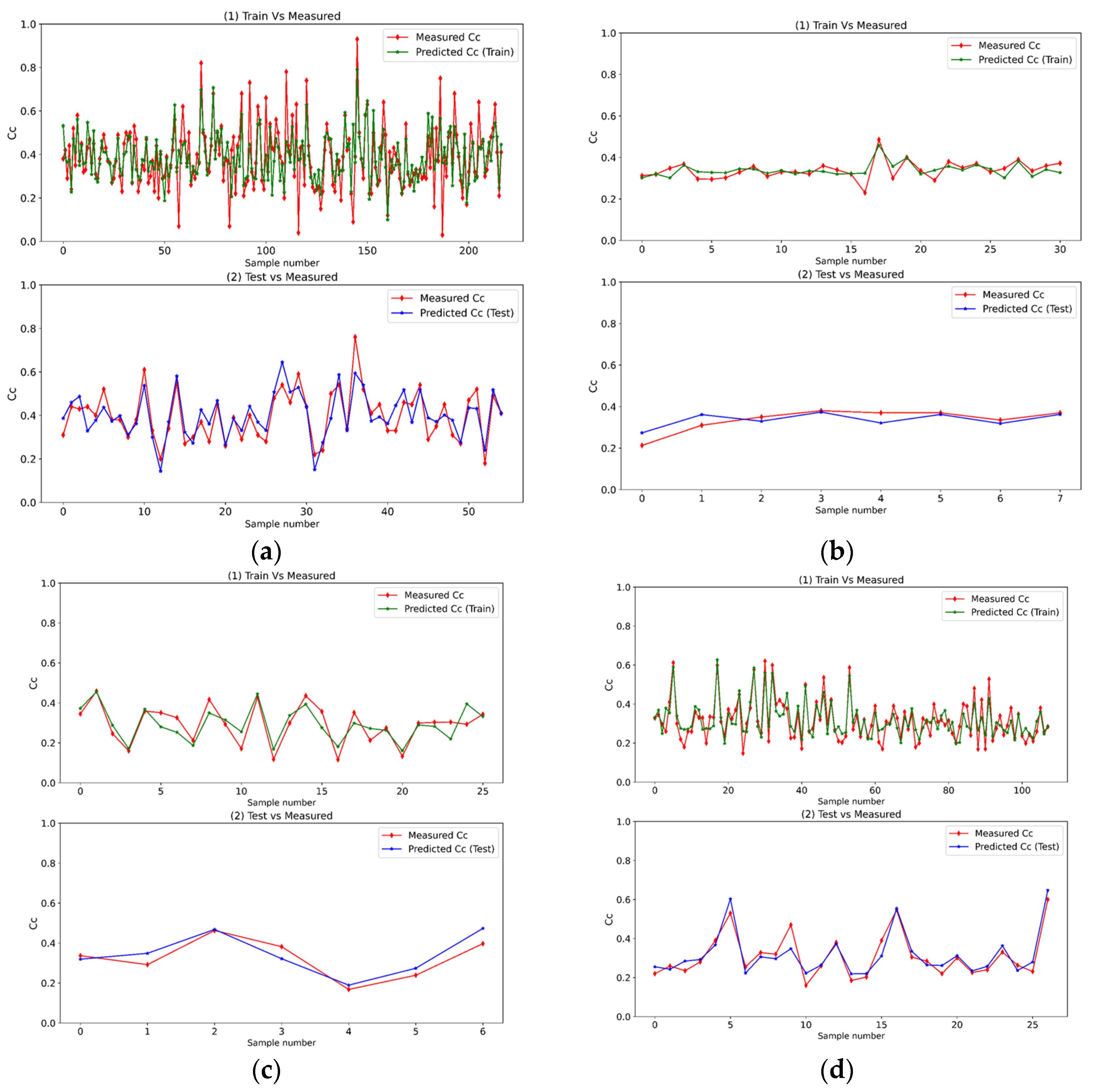
4.1. Prediction Results

The study applied four models to the entire site as well as to each classified zone. The evaluation metrics for the regression models were R² and RMSE, where an R² value closer to 1 and an RMSE closer to 0 indicate superior model performance. The ML models were optimized through hyperparameter tuning to build the most effective models.

Table 3. Performance evaluation of the C_c prediction models.

Zone		Model	Train Data		Test Data
			R2	RMSE	R2	RMSE
	Total	MLR	0.6258	0.0754	0.6742	0.0794
		RR	0.6258	0.0754	0.6742	0.0794
		LR	0.6233	0.0756	0.6699	0.08
		ENR	0.6258	0.0754	0.6741	0.0794
	Zone 1	MLR	0.5636	0.0942	0.7294	0.0591
		RR	0.5636	0.0942	0.7296	0.0591
		LR	0.5621	0.0944	0.7308	0.059
		ENR	0.5635	0.0942	0.7298	0.0591
	Zone 2	MLR	0.5002	0.0306	0.5539	0.0345
		RR	0.4707	0.0315	0.5068	0.0363
		LR	0.4177	0.033	0.4621	0.0379
		ENR	0.4181	0.033	0.4628	0.0379
	Zone 3	MLR	0.7159	0.0511	0.7575	0.0459
		RR	0.4982	0.068	0.6543	0.0548
		LR	-	-	-	-
		ENR	-	-	-	-
	Zone 4	MLR	0.7804	0.0492	0.831	0.0457
		RR	0.7765	0.0497	0.8405	0.0444
		LR	0.7695	0.0504	0.8546	0.0424
		ENR	0.7692	0.0505	0.8527	0.0427

presents the prediction results of the models for the entire site and for zones classified based on the geotechnical and hydrogeological characteristics.

When predicting the compression index for the entire site, the models generally yielded R² and RMSE values of approximately 0.67 and 0.08, respectively. Among these, the MLR model and RR model (when the hyperparameter alpha was set to 0.1) exhibited the highest R² of 0.6742.

For zone 1, located in the northern region, the average R² was approximately 0.73, and the RMSE was 0.06. Compared with the entire site, the prediction accuracy improved by about 9% based on the R² value, with minimal performance differences among the models. The highest-performing model was the LR model when alpha was set to 0.001.

For zone 2, located in the western region, the R² values ranged from 0.4621 to 0.5539, and the RMSE values ranged from 0.0345 to 0.0379, indicating the lowest predictive accuracy among the entire site and all classified zones. This is likely due to the zone being influenced by two water systems while also being located the furthest from both, resulting in a low correlation between the input data and the compression index. Among the models, the MLR model demonstrated the best prediction performance. As a result, the accuracy of the zone 2 model was found to be lower than that of the total model. Such outcomes can arise when the dataset size is not sufficiently large, potentially leading to reduced model accuracy and safety, and consequently causing various issues.

For zone 3, located in the eastern region, the R² values ranged from 0.6543 to 0.7575, and the RMSE values ranged from 0.046 to 0.055, showing an R² difference of up to 0.1 among the models. The LR and ENR models failed to produce results, likely due to the limited amount of training data, which prevented the models from accurately capturing the data distribution. Furthermore, from a hydrogeological perspective, zone 3 is influenced by both the Mangyeong River and Dongjin River, leading to a mixture of sediment characteristics. This could have hindered the model’s ability to accurately learn the data patterns. Similar to zone 2, the MLR model demonstrated a relatively better performance, which is presumed to be due to the influence of the two water systems leading to mixed geological characteristics.

For zone 4, located in the southern region, the R² values ranged from 0.831 to 0.8546, and the RMSE values ranged from 0.0424 to 0.0457, with minimal prediction accuracy differences among the models. The LR model with an alpha of 0.004 exhibited the highest accuracy.

The best model with the highest R² value for each zone was selected, and the measured and predicted values of the compression index for each data point are presented in Figure 5. Additionally, the mean absolute percentage error (MAPE) values of all models were found to follow the same trend as the RMSE values.

Considering the hydrogeological characteristics and sedimentary features of each zone, zones 1 and 4, characterized by the influence of a single hydrogeological characteristic, achieved higher prediction accuracy. In both zones, the LR model showed the best performance. On the other hand, zones 2 and 3, characterized by mixed hydrogeological influences, showed a lower prediction accuracy compared with zones 1 and 4, with the MLR model achieving a higher model performance than the LR model in these zones.

Furthermore, when zones were classified based on hydrogeological characteristics (zones 1, 3, 4), they generally exhibited higher accuracy than the case where predictions were made without considering these characteristics (total), as evaluated by R². This result confirms the importance of classifying data based on site-specific characteristics when conducting machine learning-based predictions.

Therefore, in areas characterized by mixed hydrogeological influences or insufficient training data, it is recommended to use the MLR model for predictions or to utilize the entire dataset. Conversely, in areas with clearly defined hydrogeological characteristics and simple influences, as well as abundant data, it is preferable to use the LR model or to implement the LR model after classifying the data based on geotechnical and hydrogeological characteristics.

The four ML models used in this study have the advantage of expressing the relationship between dependent and independent variables in the form of equations. Regression equations derived from the best-performing models for each zone are presented in

Table 4. Regression equations of best models by zone.

Zone	Best Model	Regression Equation	R2
1	LR	$C_c=-0.017697\left(w_n\right)+0.035058\left(\mathrm{L}\mathrm{L}\right)+0.001132\left(\mathrm{P}\mathrm{I}\right)+0.094264\left(e_0\right)+0.387972$	0.7308
2	MLR	$C_c=-0.019399\left(w_n\right)-0.008944\left(\mathrm{L}\mathrm{L}\right)+0.027466\left(\mathrm{P}\mathrm{I}\right)+0.029309\left(e_0\right)+0.339065$	0.5539
3	MLR	$C_c=-0.047816\left(w_n\right)-0.005584\left(\mathrm{L}\mathrm{L}\right)+0.044939\left(\mathrm{P}\mathrm{I}\right)+0.093734\left(e_0\right)+0.292654$	0.7575
4	LR	$C_c=0.009149\left(\mathrm{L}\mathrm{L}\right)+0.046717\left(\mathrm{P}\mathrm{I}\right)+0.038494\left(e_0\right)+0.317704$	0.8546

. The equations generated using the LR model (zones 1 and 4) showed relatively higher R² values compared with those generated using the MLR model (zones 2 and 3). In particular, the equation for zone 4 reflects the characteristics of the LR model, which eliminates less important features by setting their regression coefficients to zero. As a result, the natural water content (w_n) was excluded from the equation of zone 4. This suggests that the natural water content is a relatively less significant feature for predicting the compression index in this zone. The exclusion of the natural water content feature can be attributed to the stable sedimentation activities in areas of the Saemangeum region that are unaffected by the influences of the inner and outer seas, where the impact of natural water content on the compression index is minimal.

An analysis of the regression equations for the four zones revealed that, while the coefficients for all other soil properties consistently share the same sign, the sign of the LL coefficient varies by zone. Generally, soils with higher LL values exhibit greater compressibility. In zones 1 and 4—where a single water system predominantly influences deposition—soils are relatively homogeneous, and thus the typical geotechnical characteristic of higher LL correlating with greater compressibility is reflected, resulting in a positive LL coefficient. In contrast, zones 2 and 3, which are influenced by multiple water systems, receive sediments from diverse sources that mix and reduce overall homogeneity. Consequently, the LL coefficient in these zones appears as negative, deviating from the usual geotechnical trend. Furthermore, the LL coefficients in zones 2 and 3 are comparatively smaller than those in zones 1 and 4. In an environment with multiple water systems, the influence of LL on soil compressibility tends to be less predictable. Therefore, to reduce uncertainty, the LL coefficient is lowered, thereby minimizing its contribution to the compression index.

When comparing the absolute values of the coefficients (excluding their signs), zone 1—characterized by a homogeneous single-water-system environment with limited clay mineral diversity and a strong influence of physical structure—exhibits the initial void ratio as the most dominant property, resulting in a markedly larger coefficient gap compared with other properties. In contrast, zone 2, where diverse sediments intermix, shows the smallest difference among coefficients, indicating that all properties exert relatively similar influences on the soil. Although zone 3 is influenced by a complex water system, its proximity to land leads to a greater accumulation of coarse-grained sediments and thus a pronounced impact of physical structure. As a result, as in zone 1, the initial void ratio dominates in zone 3, producing a substantial coefficient gap relative to other properties.

4.2. Impact of Silt and Clay

The compressibility of soft ground is influenced by the silt and clay content of the soil. Therefore, to evaluate the influence of silt and clay on model performance, the relationship between the R² values across the entire site and individual zones was investigated. The R² values of the ML models calculated for each zone in Table 3, were averaged and presented in

Table 5. Mean R² value by zone.

	Zone 1	Zone 2	Zone 3	Zone 4	Saemangeum
Mean R2 Value	0.7299	0.4964	0.7059	0.8447	0.6942

.

Analyzing the prediction results based on hydrogeological characteristics shows that zone 2, located farthest from the coast, has the lowest average R² value, while zones 1, 3, and 4, closer to the coast, show higher average prediction accuracy. The average grain size of the tidal flat sediments in the Saemangeum area was the greatest in zones 1 and 4, and the smallest in zone 2. This is consistent with the trend observed in the R² values. In particular, in zone 3, an examination of the stratigraphy revealed a unique structure compared with the other zones. A thick gravel layer, 2–10 m in thickness, lay atop the bedrock layer at the bottom. Additionally, a loose sandy soil layer was deeply distributed with a thickness ranging from 1.5 to 15 m. Additionally, as shown in the investigation results presented in Figure 6, the clayey soil became thicker toward the open sea, and zone 2 had the thickest soft clay layer.

This sedimentation pattern can be attributed to the characteristics of clay and silt. Fine-grained sediments such as clay and silt, with smaller particle sizes, are more influenced by the flow and intensity of ocean currents compared with coarse-grained sediments like sand and gravel. As a result, they are transported further and deposited at greater distances. Additionally, silt and clay exhibit higher compressibility than sand and gravel, which makes their behavior more challenging to predict.

Therefore, zone 2, located farthest from the coast, featured a thick deposition of highly compressible silt and clay layers. This increased the data variability, hindered the model’s ability to learn the data distribution, and ultimately resulted in the lowest prediction accuracy.

4.3. Impact of Clay Minerals

When bedrock in a region undergoes weathering, primary minerals like feldspar and mica are produced. With further weathering, secondary minerals, including clay minerals, are generated. The type and amount of clay minerals within the soil have a significant impact on its expansiveness. Therefore, the impact of the clay mineral content and type on the performance of ML models was analyzed.

As shown in Table 5, zone 4, influenced by the Dongjin River, exhibited a higher average R² compared with zone 1, which is affected by the Mangyeong River. This difference can be attributed to variations in the bedrock underlying the two rivers. Zone 1 is influenced by the Mangyeong River, which is characterized by a mixed composition of granitic and gneissic bedrock, while zone 4 is influenced by the Dongjin River, which has granitic bedrock (Figure 2).

Kaolinite (ML), a clay mineral with the lowest activity and compressibility, is generated from primary minerals such as feldspar. In zone 4, located in the lower reaches of the Dongjin River, the predominance of granitic bedrock contains a high proportion of feldspar, a source mineral for kaolinite, resulting in low activity and high stability. In contrast, the Mangyeong River is influenced by a mixed bedrock of granite and gneiss. Gneiss, formed through metamorphism, contains a higher proportion of intergrade clay minerals comprising illite and smectite, which are more active than kaolinite.

As shown in Figure 7, zone 1, located in the lower reaches of the Mangyeong River, had higher proportions of illite (CL) and montmorillonite (CH), a highly compressible clay mineral, compared with zone 4. The high activity and compressibility of illite and montmorillonite resulted in data heterogeneity, affecting the model’s prediction accuracy and resulting in a minor decrease in R².

In the case of zone 3, being influenced by both water systems, it exhibited a middle proportion of kaolinite compared with zones 1 and 4. In zones 1, 3, and 4, a higher prediction accuracy was observed as the proportions of highly compressible and active clay minerals such as CL (illite) and CH (montmorillonite) decreased. This confirms the correlation between the characteristics of the clay minerals and model performance. However, in zone 2, as shown in Figure 6, the distribution of a thick clay layer combined with the presence of a sluice gate connected to the open sea has led to a mixture of external suspended sediments and clay layers deposited from the two water systems. This has resulted in high heterogeneity in the soil data, leading to poor model performance. The overall characteristics of each zone are presented in Figure 8.

As such, zones 1, 3, and 4, classified based on the geotechnical and hydrogeological characteristics, demonstrated a superior model performance compared with the predictions based on the entire dataset for the Saemangeum area. Notably, even with significantly smaller training datasets, sufficiently reliable model performance could be ensured by considering the geotechnical and hydrogeological characteristics. Hence, when developing models to predict the compression index of soft ground, region-specific data preprocessing should take precedence over simply increasing the quantity of data, as this approach ensures relatively stable and reliable results.

Consequently, the development of ML models for predicting the compression index of soft ground relies heavily on the distribution of data informed by the hydrogeological characteristics. When applying the average compression index values to large construction sites, it is essential to not only consider practical data acquisition, but also determine the influence range by incorporating the surrounding environmental factors including hydrogeological characteristics. This highlights the importance of data preprocessing with these considerations prior to predicting and selecting the compression index values.

5. Conclusions

This study aimed to predict the soil compression index by employing machine learning techniques that incorporate the geotechnical and hydrogeological factors, while providing a novel perspective for interpreting the results. The research focused on the Saemangeum reclaimed land, located on the west coast of South Korea, applying ML methods that incorporate geotechnical and hydrogeological factors to enhance the performance of the soil compression index prediction models.

1.

Predicting the compression index of zones classified based on the geotechnical and hydrogeological characteristics resulted in improved model performance and prediction accuracy compared with using the entire dataset.

2.

The silt and clay content of the soil significantly affected the performance of the ML models. Zone 2, which had the thickest clay layer (composed of clay and silt), experienced the lowest prediction accuracy due to its minimal hydrogeological influence and significant exposure to open-sea effects.

3.

The type of clay minerals significantly affected the performance of the ML models, and differences in the composition of clay minerals in the soil led to differences in the prediction accuracy. Notably, zones 1, 3, and 4 exhibited a higher R² compared with the predictions using the entire dataset. Additionally, zones influenced by a single water system (zones 1 and 4) demonstrated improved prediction performance, making the use of LR models more suitable. In contrast, zones influenced by multiple water systems (zones 2 and 3) showed relatively lower performance, where the use of MLR models was more appropriate.

4.

When developing machine learning models to predict the compression index for large-scale sites, it is essential to define the influence range based on the hydrogeological characteristics of the target area and perform data preprocessing in accordance with the data distribution. Subsequently, the optimal design parameters must be calculated for each defined influence range.

This study confirmed that incorporating the geotechnical and hydrogeological characteristics into the data preprocessing process can enhance the performance of ML models for predicting the compression index. However, this study focused its analysis primarily on the two main water systems, the Mangyeong River and the Dongjin River. Future studies should explore the impact of more detailed hydrological and geological characteristics on the model performance to further refine the prediction accuracy. In addition, AI has the potential to effectively analyze and train on complex and extensive data in the geotechnical field, however, the geotechnical field often involves relatively small datasets. Therefore, this study aimed to develop AI models capable of maintaining high accuracy even with limited datasets, thereby enhancing the overall accuracy and safety.

Additionally, this study explained the characteristics of the sediments in the Mangyeong and Dongjin Rivers based on the general weathering properties of the bedrock. However, the soil formation of a parent rock is influenced by numerous factors including the region’s climate, topography, and vegetation. Considering these factors could provide a more precise perspective of how the hydrological and sedimentary characteristics affect the performance of ML models.

References

1. Singh, S. A Review on Trends in Ground Improvement Techniques. J. Geotech. Eng. 2018, 5, 18–22. [Google Scholar] [CrossRef]
2. Gouw, T.L.; Gunawan, A. Vacuum Preloading, an alternative soft ground improvement technique for a sustainable development. IOP Conf. Ser. Earth Environ. Sci. 2020, 426, 012003. [Google Scholar] [CrossRef]
3. Oda, K.; Yokota, K.; Bu, L.D. Stochastic estimation of consolidation settlement of soft clay layer with Artificial Neural Network. Jpn. Geotech. Soc. Spec. Publ. 2016, 2, 2529–2534. [Google Scholar] [CrossRef]
4. KDS 44 30 00 Road Earthworks; Ministry of Land, Infrastructure and Transport: Sejong, Republic of Korea, 2022. (In Korean)
5. Boulanger, R.W.; Idriss, I.M. Liquefaction susceptibility criteria for silts and clays. J. Geotech. Geoenviron. Eng. 2006, 132, 1413–1426. [Google Scholar] [CrossRef]
6. Ural, N. The importance of clay in geotechnical engineering. In Current Topics in the Utilization of Clay in Industrial and Medical Applications; IntechOpen: London, UK, 2018. [Google Scholar]
7. Younis, S.N.; Mahmood, R.A.; Alsaad, H.A. Swelling potential and mineralogy of al-Hartha City soil in Basrah-Southern Iraq. Iraqi J. Sci. 2024, 65, 2020–2030. [Google Scholar] [CrossRef]
8. Firoozi, A.A.; Firoozi, A.A.; Baghini, M.S. A review of clayey soils. Asian J. Appl. Sci. 2016, 4, 1319–1330. [Google Scholar]
9. Analysis of Ground Settlement and Deformation Behavior of Civil Engineering Structures; Korea National Housing Corporation: Jinju-si, Republic of Korea, 1994. (In Korean)
10. Trinh Dinh, T. A study on settlements of road embankments on soft ground using vertical drains. Transp. Commun. Sci. J. 2024, 75, 1477–1488. [Google Scholar] [CrossRef]
11. Kurnaz, T.F.; Dagdeviren, U.; Yildiz, M.; Ozkan, O. Prediction of compressibility parameters of the soils using artificial neural network. SpringerPlus 2016, 5, 1801. [Google Scholar] [CrossRef]
12. Bardhan, A.; Kardani, N.; Alzo’ubi, A.K.; Samui, P.; Gandomi, A.H.; Gokceoglu, C. A comparative analysis of hybrid computational models constructed with swarm intelligence algorithms for estimating soil compression index. Arch. Comput. Method Eng. 2022, 29, 4735–4773. [Google Scholar] [CrossRef]
13. Azzouz, A.S.; Krizek, R.J.; Corotis, R.B. Regression analysis of soil compressibility. Soils Found. 1976, 16, 19–29. [Google Scholar] [CrossRef]
14. Rendon-Herrero, O. Universal compression index equation. J. Geotech. Eng. Div. 1980, 106, 1179–1200. [Google Scholar] [CrossRef]
15. Koppula, S. Statistical estimation of compression index. Geotech. Test. J. 1981, 4, 68–73. [Google Scholar] [CrossRef]
16. Park, H.I.; Lee, S.R. Evaluation of the compression index of soils using an artificial neural network. Comput. Geotech. 2011, 38, 472–481. [Google Scholar] [CrossRef]
17. Kalantary, F.; Kordnaeij, A. Prediction of compression index using artificial neural network. Sci. Res. Essays 2012, 7, 2835–2848. [Google Scholar] [CrossRef]
18. Nishida, Y. A brief note on Compression Index of Soil. J. Soil Mech. Found. Div. 1956, 82, 1–14. [Google Scholar] [CrossRef]
19. Gunduz, Z.; Arman, H. Possible relationships between compression and recompression indices of a low-plasticity clayey soil. Arab. J. Sci. Eng. 2007, 32, 179–190. [Google Scholar]
20. Terzaghi, K.; Peck, R.B.; Mesri, G. Soil Mechanics in Engineering Practice; John Wiley & Sons: New York, NY, USA, 1996. [Google Scholar]
21. Kulkarni, M.P.; Patel, A.; Singh, D.N. Application of shear wave velocity for characterizing clays from coastal regions. KSCE J. Civ. Eng. 2010, 14, 307–321. [Google Scholar] [CrossRef]
22. Alizadeh Majdi, A.; Dabiri, R.; Ganjian, N.; Ghalandarzadeh, A. Determination of the soil compression index (CC) in clayey soils using shear wave velocity (Case study: Tabriz city). Iran. J. Sci. Technol. Trans. Civ. Eng. 2018, 43, 577–588. [Google Scholar] [CrossRef]
23. Al-Khafaji, A.W.; Andersland, O.B. Equations for compression index approximation. J. Geotech. Eng. ASCE 1992, 118, 148–153. [Google Scholar] [CrossRef]
24. Ozer, M.; Isik, N.S.; Orhan, M. Statistical and neural network assessment of the compression index of clay-bearing soils. Bull. Eng. Geol. Environ. 2008, 67, 537–545. [Google Scholar] [CrossRef]
25. Yoon, G.L.; Kim, B.T. Regression analysis of compression index for Kwangyang Marine Clay. KSCE J. Civ. Eng. 2006, 10, 415–418. [Google Scholar] [CrossRef]
26. Ibrahim, D. An overview of soft computing. Procedia Comput. Sci. 2016, 102, 34–38. [Google Scholar] [CrossRef]
27. Mamudur, K.; Kattamuri, M.R. Application of boosting-based ensemble learning method for the prediction of compression index. J. Inst. Eng. (India) Ser. A 2020, 101, 409–419. [Google Scholar] [CrossRef]
28. Long, T.; He, B.; Ghorbani, A.; Khatami, S.M.H. Tree-based techniques for predicting the compression index of clayey soils. J. Soft Comput. Civ. Eng. 2023, 7, 52–67. [Google Scholar] [CrossRef]
29. Lee, S.; Kang, J.; Kim, J.; Baek, W.; Yoon, H. A study on developing a model for predicting the compression index of the South Coast Clay of korea using statistical analysis and Machine Learning Techniques. Appl. Sci. 2024, 14, 952. [Google Scholar] [CrossRef]
30. Kumar, V.P.; Rani, C.S. Prediction of compression index of soils using artificial neural networks (ANNs). Int. J. Eng. Res. Appl. 2011, 1, 1554–1558. [Google Scholar]
31. Al-Taie, A.J.; Al-Bayati, A.F.; Taki, Z.N. Compression index and compression ratio prediction by Artificial Neural Networks. J. Eng. 2017, 23, 96–106. [Google Scholar] [CrossRef]
32. Zhang, P.; Yin, Z.Y.; Jin, Y.F.; Chan, T.H.T.; Gao, F.P. Intelligent modelling of clay compressibility using hybrid meta-heuristic and machine learning algorithms. Geosci. Front. 2021, 12, 441–452. [Google Scholar] [CrossRef]
33. Díaz, E.; Spagnoli, G. A super-learner machine learning model for a global prediction of compression index in Clays. Appl. Clay Sci. 2024, 249, 107239. [Google Scholar] [CrossRef]
34. Final Design Report for the Saemangeum East-West Axis 2 Road Construction Project (Section 1); Saemangeum Development and Investment Agency: Gunsan-si, Republic of Korea, 2015. (In Korean)
35. Lee, H.J.; Jo, H.R.; Kim, M.J. Topographical changes and textural characteristics in the areas around the Saemangeum dyke. Ocean Polar Res. 2006, 28, 293–303. (In Korean) [Google Scholar] [CrossRef]
36. Park, Y.A.; Kang, H.J.; Song, Y.I. Sandy sediment transport mechanism on tidal sand bodies, west coast of Korea. Korean J. Quat. Res. 1991, 5, 33–45. [Google Scholar]
37. Choi, H.Y. Constitutive Characteristics Among Saemangeum Soft Ground. Master’s Thesis, Chung-Ang University, Seoul, Republic of Korea, 2023. [Google Scholar]
38. Final Design Geotechnical Investigation Report for the Saemangeum East-West Axis 2 Road Construction Project (Section 1); Saemangeum Development and Investment Agency: Gunsan-si, Republic of Korea, 2015. (In Korean)
39. Geotechnical Investigation Report for the Saemangeum East-West Axis 2 Road Construction Project (Section 2); Saemangeum Development and Investment Agency: Gunsan-si, Republic of Korea, 2015. (In Korean)
40. Geotechnical Investigation Report for the Second Phase (Section 1) of the Saemangeum North-South Road Construction Project; Saemangeum Development and Investment Agency: Gunsan-si, Republic of Korea, 2018. (In Korean)
41. Final Design Report for the Second Phase (Section 1) of the Saemangeum North-South Road Construction Project; Saemangeum Development and Investment Agency: Gunsan-si, Republic of Korea, 2018. (In Korean)
42. Geotechnical Investigation Report for the Second Phase (Section 2) of the Saemangeum North-South Road Construction Project; Saemangeum Development and Investment Agency: Gunsan-si, Republic of Korea, 2018. (In Korean)
43. Final Design Report for the Second Phase (Section 2) of the Saemangeum North-South Road Construction Project; Saemangeum Development and Investment Agency: Gunsan-si, Republic of Korea, 2018. (In Korean)
44. Geotechnical Investigation Report for the Second Phase (Section 4) of the Saemangeum North-South Road Construction Project; Saemangeum Development and Investment Agency: Gunsan-si, Republic of Korea, 2017. (In Korean)
45. Soil Investigation Report for the Saemangeum District Industrial Complex Development Project; Korea Rural Community Corporation: Naju-si, Republic of Korea, 2010. (In Korean)
46. Geological and Material Source Investigation Report for the Saemangeum Smart Waterfront City Reclamation Project; Saemangeum Development and Investment Agency: Gunsan-si, Republic of Korea, 2021. (In Korean)
47. Final Design Report for the Saemangeum Smart Waterfront City Reclamation Project; Saemangeum Development and Investment Agency: Gunsan-si, Republic of Korea, 2021. (In Korean)
48. Bourouis, M.A.; Zadjaoui, A.; Djedid, A. The Neuro-genetic approach for estimating the compression index. J. Mater. Eng. Struct. 2018, 5, 305–315. [Google Scholar]
49. Marill, K.A. Advanced statistics: Linear regression, part II: Multiple linear regression. Acad. Emerg. Med. 2004, 11, 94–102. [Google Scholar] [CrossRef] [PubMed]
50. Farahani, H.A.; Rahiminezhad, A.; Same, L. A comparison of partial least squares (PLS) and ordinary least squares (OLS) regressions in predicting of couples mental health based on their communicational patterns. Procedia Soc. Behav. Sci. 2010, 5, 1459–1463. [Google Scholar] [CrossRef]
51. Géron, A. Hands-On Machine Learning with Scikit-Learn, Keras and Tensorflow; O’Reilly Media Inc.: Sebastopol, CA, USA, 2023. [Google Scholar]
52. García-Nieto, P.J.; García-Gonzalo, E.; Paredes-Sánchez, J.P. Prediction of the critical temperature of a superconductor by using the WOA/Mars, Ridge, lasso and elastic-net machine learning techniques. Neural Comput. Appl. 2021, 33, 17131–17145. [Google Scholar] [CrossRef]
53. Al-Obeidat, F.; Spencer, B.; Alfandi, O. Consistently accurate forecasts of temperature within buildings from sensor data using ridge and lasso regression. Future Gener. Comput. Syst. 2020, 110, 382–392. [Google Scholar] [CrossRef]
54. Raschka, S.; Mirjalili, V. Python Machine Learning: Machine Learning and Deep Learning with Python, Scikit-Learn, and Tensorflow 2; Packt Publishing: Birmingham, UK, 2019. [Google Scholar]
55. Tibshirani, R. Regression shrinkage and selection via the lasso. J. R. Stat. Soc. Ser. B Stat. Methodol. 1996, 58, 267–288. [Google Scholar] [CrossRef]
56. Wang, S.; Ji, B.; Zhao, J.; Liu, W.; Xu, T. Predicting ship fuel consumption based on lasso regression. Transport. Res. Part D-Transport. Environ. 2018, 65, 817–824. [Google Scholar] [CrossRef]
57. Chen, J.; de Hoogh, K.; Gulliver, J.; Hoffmann, B.; Hertel, O.; Ketzel, M.; Bauwelinck, M.; Van Donkelaar, A.; Hvidtfeldt, U.A.; Katsouyanni, K.; et al. A comparison of linear regression, regularization, and machine learning algorithms to develop Europe-wide spatial models of fine particles and Nitrogen Dioxide. Environ. Int. 2019, 130, 104934. [Google Scholar] [CrossRef]
58. Zou, H.; Hastie, T. Regularization and variable selection via the elastic net. J. R. Stat. Soc. Ser. B Stat. Methodol. 2005, 67, 301–320. [Google Scholar] [CrossRef]
Figure 1. Satellite image of the Saemangeum reclaimed tidal land [37].
Applsci 15 02757 g001
Figure 2. Geological map of the Saemangeum reclaimed land [34].
Applsci 15 02757 g002
Figure 3. Zone classification of the Saemangeum reclaimed land.
Applsci 15 02757 g003
Figure 4. ML flowchart.
Applsci 15 02757 g004
Figure 5. Actual and predicted values for best models. (a) Zone 1 (LR); (b) Zone 2 (MLR); (c) Zone 3 (MLR); (d) Zone 4 (LR).
Applsci 15 02757 g005
Figure 6. Distribution of the soft clay layer.
Applsci 15 02757 g006
Figure 7. The proportion of clay minerals by zone. (a) Zone 1; (b) zone 2; (c) zone 3; (d) zone 4.
Applsci 15 02757 g007
Figure 8. Characteristics by zone.
Applsci 15 02757 g008