Power Quality Disturbance Classification Method Based on Unscented Kalman Filter and Kernel Extreme Learning Machine

Abstract

The power quality index is an important index in the power industry. Power quality disturbances (PQDs) have a great impact on the power grid. It is important to identify the type of PQDs accurately. However, it is difficult to analyze a large number of PQDs, especially in more complex power systems. Considering the limitations of the traditional time–frequency domain method and the complexity of the optimization algorithm in extracting features, a novel algorithm is proposed to classify the PQDs in this paper, which is based on the unscented Kalman filter (UKF) and the kernel extreme learning machine (KELM). The UKF is used to detect and process the original disturbances, and anti-noise detection performance is analyzed by tracking the amplitude change in voltage swell under different signal–noise ratios (SNRs). The amplitudes of the fundamental wave, third harmonic, fifth harmonic, seventh harmonic, and oscillatory wave are tracked in real time, and their minimum and peak indexes are taken as the optimal feature vector set. The feature vector set is classified by the KELM. The performance of the proposed method has also been evaluated with simulated and experimental results.

1. Introduction

In recent years, with the increasing development of the smart grid, ensuing energy quality disturbance problems have emerged in an endless stream, which has a great impact on the safety, efficiency, and economy of the overall operation of the power grid. Every year, the economic losses caused by power quality problems are as high as hundreds of millions of Chinese yuan worldwide. Therefore, improving power quality problems has far-reaching significance for the overall safety and stability of the power grid as well as economic benefits [1,2,3]. It is particularly important to track, monitor, and analyze the power quality of the power grid.

At present, the parameter estimation methods for PQDs detection and processing include singular value decomposition (SVD) [4,5], short-time Fourier transform (STFT) [6,7], wavelet transform (WT) [8,9,10], Kalman filtering (KF) [11,12,13], Hilbert–Huang transform (HHT) [14], compressed sensing, (CS) [15], phase space reconstruction (PSR) [16], and so on. Because there are obvious singular values near the mutation point of the power quality transient disturbance, SVD becomes an effective method to deal with this kind of signal. However, the results of this time domain analysis method lack the description of the frequency domain characteristics of the signal, which has certain limitations. STFT can obtain better detection results by selecting the appropriate window function, but due to the fixed window function selection of STFT in time and frequency, it is not suitable for the detection of transient disturbances. On the basis of STFT, WT can adaptively change the window function by introducing scale and translation factors, so that WT is suitable for analyzing the power quality transient disturbances. However, the results of WT are easily affected by the selection of the wavelet basis and the number of decomposition layers. KF is a signal processing method based on state space estimation. By decomposing the PQDs into a constant component and a fluctuation component, the amplitude, phase, and frequency can be accurately estimated. On the basis of KF, a harmonic detection method based on the maximum likelihood of Kalman filter residual analysis is proposed in [11], which can accurately detect the start and end time of harmonic. Hilbert–Huang transform is a new time–frequency analysis method suitable for non-stationary and nonlinear signals in recent years. It is mainly composed of empirical mode decomposition (EMD) and Hilbert transform. Because the intrinsic mode function (IMF) extraction of the EMD method is a time–frequency analysis process based on the local characteristic time scale of the signal, it is easy to have endpoint effects and modal aliasing problems for transient oscillation.

Compressed sensing (CS) is a signal processing technique that enables efficient signal reconstruction using a reduced number of samples by exploiting the sparsity of the signal. In power quality disturbance classification, CS can significantly reduce data dimensionality and computational burden, thereby improving detection efficiency. However, CS assumes that the signal is sparse, which may lead to reduced reconstruction accuracy when the disturbance signals are complex or non-sparse, thus affecting classification performance. To address these issues, the literature [15] proposes combining CS with deep learning techniques, such as deep convolutional neural networks (CNNs), to enhance the robustness and accuracy of the disturbance classification, even in the presence of non-sparse signals. This hybrid approach leverages the strengths of both CS and CNNs, resulting in improved classification performance and efficiency.

Phase space reconstruction (PSR) is a technique for extracting dynamic features from time series data by constructing a phase space, which helps reveal the nonlinear and time-varying characteristics of power quality disturbance signals. PSR provides a comprehensive view of the system’s dynamics, making it well-suited for analyzing complex disturbance signals. However, its effectiveness heavily relies on the choice of embedding dimension and time delay, and it can be sensitive to high noise levels, potentially affecting classification accuracy. In reference [16], the authors combine PSR with convolutional neural networks (CNN) to enhance the classification performance of power quality disturbance signals. First, PSR extracts dynamic features from the signal, capturing its nonlinear and time-varying characteristics. These features are then fed into the CNN, which leverages its deep learning capabilities to further refine and extract effective classification features. The combination of PSR and CNN improves classification accuracy, particularly in noisy and complex scenarios, demonstrating enhanced robustness.

The results of PQDs signal detection and analysis cannot be directly classified, so the feature set related to signal processing results needs to be extracted. At present, the artificial intelligence methods for screening and optimizing feature sets mainly include the genetic algorithm, particle swarm optimization, simulated annealing, wolf pack algorithm, random forest, and so on. Through the artificial intelligence algorithms listed above, the optimal feature vector combination can be found [17,18]. An ML-DT algorithm has been proposed based on single-label decision tree extension to support multi-label data sets in [17]. With this algorithm, a random forest classifier, ML-RF, was constructed. By applying the ML-RF algorithm, PQDs can be classified. In addition, common methods include support vector machine, artificial neural network, deep learning [19,20], and so on.

Considering the limitations of the traditional time–frequency domain method and the complexity of the optimization algorithm in extracting features, a detection and classification method combining the unscented Kalman filter (UKF) and the kernel extreme learning machine (KELM) is proposed for the classification of PQDs in this paper. The UKF is used to detect and process the original disturbances, and the optimal feature vector set is selected. The classification of single or composite PQD types is completed by the kernel extreme learning machine. The UKF-KELM classification method is used to track the disturbances in the experimental platform of the PQD classification, and the classification of PQDs is completed. The experimental results show that the classification method in this paper has a high degree of fit, strong effectiveness, and high accuracy.

This paper is structured as follows: Section 2 presents the unscented Kalman filter (UKF) for detecting power quality disturbances (PQDs), with Section 2.1 describing the methodology of the UKF and Section 2.2 analyzing its anti-noise detection performance. Section 3 focuses on the feature extraction techniques used for PQDs. Section 4 introduces the kernel extreme learning machine (KELM) method applied to PQDs classification. Section 5 provides experimental verification of the proposed approach, and Section 6 concludes the paper with a summary of the findings and potential future work.

2. The UKF Detection of PQDs

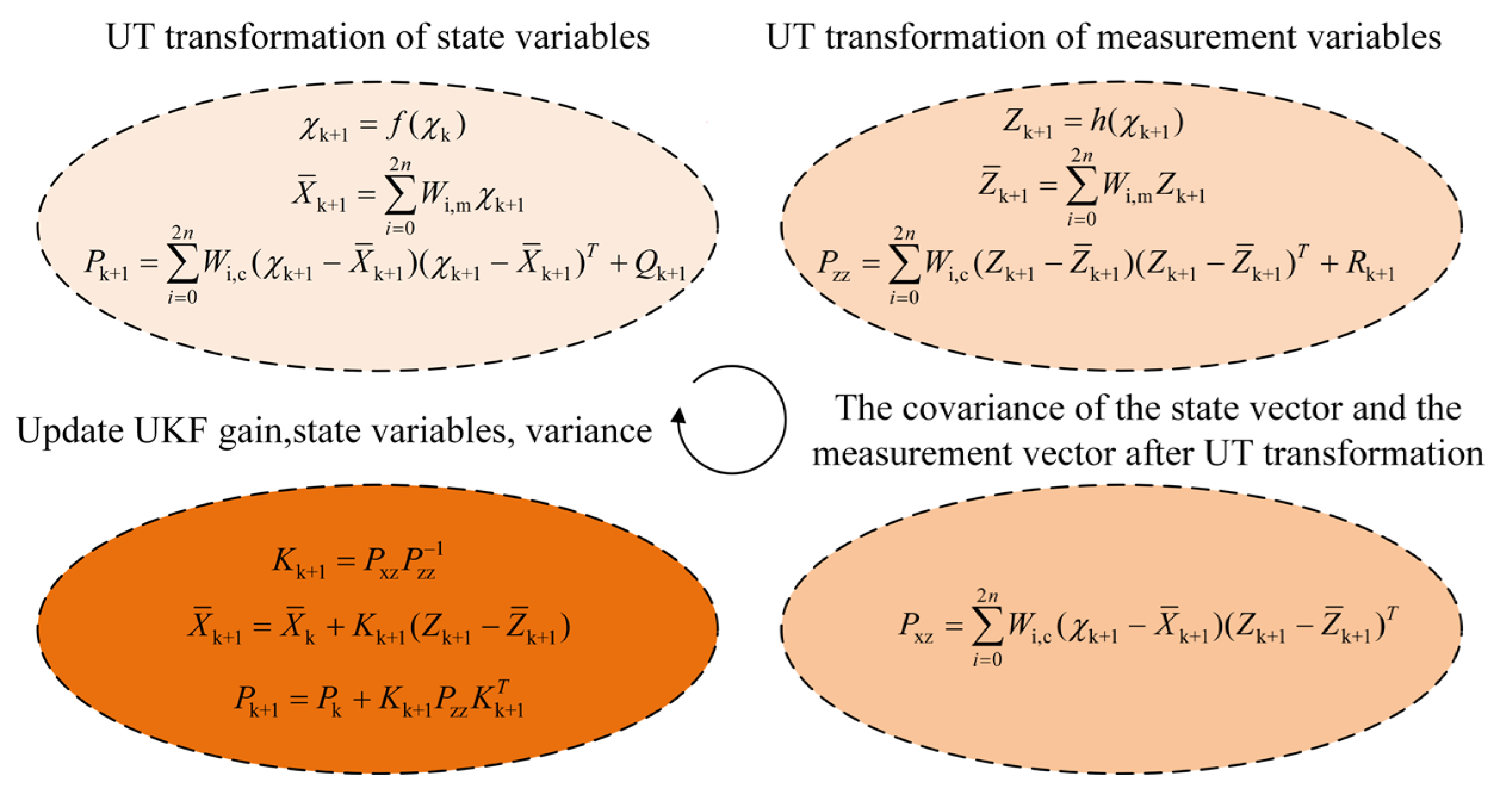
2.1. Unscented Kalman Filter

The state space equations of nonlinear discrete systems are described as follows:

$$X_{\mathrm{k}+1}=f(X_{\mathrm{k}})+W_{\mathrm{k}}$$

(1)

$$Z_{\mathrm{k}}=\Psi ({\overline{X}}_{\mathrm{k}})+V_{\mathrm{k}}$$

(2)

where $X_{\mathrm{k}+1}$ is state vector, $Z_{\mathrm{k}}$ is measurement vector, $f(\cdot ),\Psi (\cdot )$ is a nonlinear transformation and a nonlinear function satisfied by the system. $W_{\mathrm{k}}$ is a process noise, $V_{\mathrm{k}}$ is measurement noise. $W_{\mathrm{k}}~N\left(0,Q\right),V_{\mathrm{k}}~N\left(0,R\right)$, where N represents the normal distribution, $W_{\mathrm{k}}$ and $V_{\mathrm{k}}$ follow normal distributions with means of 0 and covariances of $Q$ and $R$, respectively. The mathematical modeling of the UKF is divided into the following six steps:

• Step 1: Define initialization state

${\overline{X}}_0$ and Variance matrix $P_0$ as follows:

$${\overline{X}}_0=E(X_0)$$

(3)

$$P_0=E[(X_0-{\overline{X}}_0){(X_0-{\overline{X}}_0)}^T]$$

(4)

where $E(\cdot )$ is the expectation operator used to describe the mean of a random variable.

• Step 2: Sigma Point Sampling for State Variables

Sigma points are used in the UKF to represent the distribution of the state vector. They are generated by adding and subtracting the square root of the weighted covariance matrix from the current state mean. Sigma points effectively capture the state distribution under nonlinear transformations. The calculation process is shown in Equation (5), which generates the first sigma point, sigma points from 1 to n, and sigma points from n + 1 to 2n.

$${\chi }_{\mathrm{i}}=\left\{\begin{array}{l}\begin{array}{cc}\overline{x}& i=0\end{array}\\ \begin{array}{cc}\overline{x}+{[\sqrt{(n+\lambda )P_{\mathrm{x}}}]}_{\mathrm{i}}& i=1,2,\dots ,n\end{array}\\ \begin{array}{cc}\overline{x}-{[\sqrt{(n+\lambda )P_{\mathrm{x}}}]}_{\mathrm{i}}& i=n+1,n+2,\dots ,2n\end{array}\end{array}\right.$$

(5)

where λ is the scale factor, ${(\sqrt{P})}^T(\sqrt{P})=P$, $P$ is the covariance matrix, ${(\sqrt{P})}_{\mathrm{i}}$ is the i-th column of the root of the matrix.

• Step 3: Complete the sigma sampling point nonlinear conversion of state variables using the following equation:

$${\chi }_{\mathrm{k}+1}=f({\chi }_{\mathrm{k}})$$

(6)

$${\overline{X}}_{\mathrm{k}+1}={\displaystyle \sum _{i=0}^{2n}{W}_{\mathrm{i},\mathrm{m}}{\chi }_{\mathrm{k}+1}}$$

(7)

$$P_{\mathrm{k}+1}={\displaystyle \sum _{i=0}^{2n}{W}_{\mathrm{i},\mathrm{c}}({\chi }_{\mathrm{k}+1}-{\overline{X}}_{\mathrm{k}+1})}{({\chi }_{\mathrm{k}+1}-{\overline{X}}_{\mathrm{k}+1})}^T+Q_{\mathrm{k}+1}$$

(8)

where $Q_{\mathrm{k}+1}$ is the covariance matrix of process noise $W_{\mathrm{k}}$ at time k + 1; $W_{i,c}$ is the weight coefficient of the ith Sigma point when the state is updated; $W_{\mathrm{i},\mathrm{m}}$ is the weight coefficient of the ith Sigma point when the measurement is updated.

• Step 4: Complete nonlinear conversion of sigma sampling points for measurement using the following equation:

$${\chi }_{\mathrm{i}}=\left\{\begin{array}{l}\begin{array}{cc}\overline{x}& i=0\end{array}\\ \begin{array}{ll}\overline{x}+{[\sqrt{(n+\lambda )P_{\mathrm{x}}}]}_{\mathrm{i}}& i=1,2,\dots ,n\end{array}\\ \begin{array}{ll}\overline{x}-{[\sqrt{(n+\lambda )P_{\mathrm{x}}}]}_{\mathrm{i}}& i=n+1,n+2,\dots ,2n\end{array}\end{array}\right.$$

(9)

$$Z_{\mathrm{k}+1}=\Psi ({\chi }_{\mathrm{k}+1})$$

(10)

$${\overline{Z}}_{\mathrm{k}+1}={\displaystyle \sum _{i=0}^{2n}{W}_{\mathrm{i},\mathrm{m}}{Z}_{\mathrm{k}+1}}$$

(11)

$$P_{\mathrm{zz}}={\displaystyle \sum _{i=0}^{2n}{W}_{\mathrm{i},\mathrm{c}}(Z_{\mathrm{k}+1}-{\overline{Z}}_{\mathrm{k}+1})}{(Z_{\mathrm{k}+1}-{\overline{Z}}_{\mathrm{k}+1})}^T+R_{\mathrm{k}+1}$$

(12)

where $R_{\mathrm{k}+1}$ is the covariance matrix of measurement noise $V_{\mathrm{k}}$ at time k + 1.

• Step 5: The covariance between the state vector and the measurement vector is described as follows:

$$P_{\mathrm{x}\mathrm{z}}={\displaystyle \sum _{i=0}^{2n}{W}_{\mathrm{i},\mathrm{c}}({\chi }_{\mathrm{k}+1}-{\overline{X}}_{\mathrm{k}+1})}{(Z_{\mathrm{k}+1}-{\overline{Z}}_{\mathrm{k}+1})}^T$$

(13)

• Step 6: The UKF gain is calculated, the state vector and variance are updated by the following:

$$k_{\mathrm{k}+1}=P_{\mathrm{x}\mathrm{z}}{P}_{\mathrm{zz}}^{-1}$$

(14)

$${\overline{X}}_{\mathrm{k}+1}={\overline{X}}_{\mathrm{k}}+k_{\mathrm{k}+1}(Z_{\mathrm{k}+1}-{\overline{Z}}_{\mathrm{k}+1})$$

(15)

$$P_{\mathrm{k}+1}=P_{\mathrm{k}}+k_{\mathrm{k}+1}{P}_{\mathrm{z}\mathrm{z}}{k}_{\mathrm{k}+1}^T$$

(16)

where $P_{\mathrm{x}\mathrm{z}}$ is the covariance matrix between the state and the measurement; $P_{\mathrm{z}\mathrm{z}}$ is the covariance matrix of the observation vector itself.

Compared with the traditional KF, which needs to solve the Jacobian matrix, UKF does not need to solve the matrix, which makes UKF more efficient and can avoid numerical calculation errors. The flowchart of UKF is shown in Figure 1. In this flowchart, the UKF process proceeds through four steps in a loop. First, Sigma points are generated from the current state estimate and transformed through the Unscented Transform (UT) to obtain the predicted state variables. Then, these Sigma points are passed through the measurement equation to obtain the predicted measurement variables. Next, based on the predicted state and measurement, the Kalman gain is calculated and used to update the state estimate and covariance. Finally, the covariance between the state and measurement is updated based on the latest Sigma points. This process is repeated at each time step to continuously improve the state estimation of the system.

2.2. Analysis of Anti-Noise Detection Performance

Referring to the data in [21], the PQD data set was obtained from matlab 2020. The total sampling time is set to 0.2 s, the sampling frequency is 10 kHz, the sampling interval is 0.1 ms, the frequency of the voltage signal is 50 Hz, and the period is 0.02 s. The voltage amplitude is normalized. UKF is used to track the amplitude change in voltage swell under different signal–noise ratios (SNRs). Figure 2a,b are 40 db and 20 db, respectively. The red curve represents the theoretical value, the black curve is the UKF tracking result, and the pink rectangular area is the rise or fall adjustment time span of the filter waveform curve. It can be seen from the diagram that as the signal-to-noise ratio decreases, the interference of the waveform tracking curve becomes larger and larger, and the waveform rise or fall span gradually becomes larger.

In order to further compare the performance of signal detection methods, the quantitative analysis and comparison of each index of KF and UKF in tracking and detecting voltage swell are carried out.

The root mean square error of the amplitude is defined as follows:

$$e_{\mathrm{R}\mathrm{M}\mathrm{S}\mathrm{E}}=\sqrt{{\displaystyle \frac{1}{m}}{\displaystyle \sum _{\mathrm{k}=1}^m{(x_{\mathrm{k}}-{\overline{x}}_{\mathrm{k}})}^2}}$$

(17)

The mean absolute error of the amplitude is defined as follows:

$$e_{\mathrm{MAE}}={\displaystyle \frac{1}{m}}{\displaystyle \sum _{\mathrm{k}=1}^m\left|x_{\mathrm{k}}-{\overline{x}}_{\mathrm{k}}\right|}$$

(18)

where m is the total sampling points, $x_{\mathrm{k}}$ is the state estimation value, and ${\overline{x}}_{\mathrm{k}}$ is actual value of state. The performance comparison of KF and UKF for PQDs is shown in

Table 1. Comparison of KF and UKF performance.

Algorithm	SNR	${\mathit{e}}_{\mathbf{R}\mathbf{M}\mathbf{S}\mathbf{E}}$	${\mathit{e}}_{\mathbf{MAE}}$
KF	15	0.0206	0.0809
	25	0.0100	0.0404
	35	0.0087	0.0280
UKF	15	0.0149	0.0765
	25	0.0092	0.0387
	35	0.0085	0.0274

.

It can be seen that the root mean square error and the mean absolute error of UKF for voltage swell tracking curve estimation are less than KF under the same SNR environment in Table 1. As the SNR increases, the corresponding root mean square error and mean absolute error gradually decrease, which is consistent with the theoretical analysis. Therefore, UKF has better robustness and can better handle interference and noise. The mathematical expression and parameter constraints of PQD in this paper are shown in

Table 2. The mathematical models of fourteen kinds of PQDs events.

Label	Events	Mathematical Equations	Parameters Limits
C1	Swell	$y(t)=\{1+\beta [u(t-t_1)-u(t-t_2)]\}\sin (\omega t)$	$\begin{array}{c}\beta =0.1~0.9,\\ T<t_2-t_1<8T\end{array}$
C2	Sag	$y(t)=\{1-\beta [u(t-t_1)-u(t-t_2)]\}\sin (\omega t)$	$\begin{array}{c}\beta =0.1~0.9,\\ T<t_2-t_1<8T\end{array}$
C3	Interruption	$y(t)=\{1-\beta [u(t-t_1)-u(t-t_2)]\}\sin (\omega t)$	$\begin{array}{c}\beta =0.9~1,\\ T<t_2-t_1<8T\end{array}$
C4	Fluctuations	$y(t)=\{1+{\alpha }_{\mathrm{f}}\sin ({\beta }_{\mathrm{f}}\omega t)\}\sin (\omega t)$	$\begin{array}{l}{\alpha }_{\mathrm{f}}=0.1~0.3,\\ {\beta }_{\mathrm{f}}=0.1~0.5\end{array}$
C5	Pulse	$y(t)=\sin (\omega t)+\beta [u(t-t_1)-u(t-t_2)]$	$\begin{array}{c}\beta =1~3,\\ 1 \mathrm{ms}\le t_2-t_1\le 3 \mathrm{ms}\end{array}$
C6	Oscillatory	$y(t)=\sin (\omega t)+\lambda e^{-(t-t_1)/\tau }\sin \mu \omega (t-t_1)[u(t-t_1)-u(t-t_2)]$	$\begin{array}{c}\lambda =0.1~0.8,\\ \mu =10~40,\\ 0.5T<t_2-t_1<3T\end{array}$
C7	Harmonics	$y(t)=\sin (\omega t)+{{\displaystyle \sum }}_{i=3,n=1}^{2n+1}{b}_i\sin \left(i\omega (t-t_1)\right)$	$\begin{array}{c}1\le n\le 3,\\ i=3,5,7\end{array}$
C8	Harmonics + Swell	$y(t)=\{1+\beta [u(t-t_1)-u(t-t_2)]\}\sin (\omega t)+{{\displaystyle \sum }}_{i=3,n=1}^{2n+1}{b}_{\mathrm{i}}\sin \left(i\omega (t-t_3)\right)$	$\begin{array}{c}\beta =0.1~0.9,\\ T<t_2-t_1<8T\end{array}$$1\le n\le 3,i=3,5,7$
C9	Harmonics + Sag	$y(t)=\{1-\beta [u(t-t_1)-u(t-t_2)]\}\sin (\omega t)+{{\displaystyle \sum }}_{i=3,n=1}^{2n+1}{b}_{\mathrm{i}}\sin \left(i\omega (t-t_3)\right)$	$\begin{array}{c}\beta =0.1~0.9,\\ T<t_2-t_1<8T,\end{array}$$1\le n\le 3,i=3,5,7$
C10	Oscillatory + Sag	$\begin{array}{l}y(t)=\{1-\beta [u(t-t_1)-u(t-t_2)]\}\sin (\omega t)\\ +\lambda e^{-(t-t_3)/\tau }\sin \mu \omega (t-t_3)[u(t-t_3)-u(t-t_4)]\end{array}$	$\begin{array}{c}\beta =0.1~0.9,\\ T<t_2-t_1<8T,\end{array}$$\begin{array}{c}\lambda =0.1~0.8,\\ \mu =10~40,\\ 0.5T<t_4-t_3<3T\end{array}$
C11	Oscillatory + Interruption	$\begin{array}{l}y(t)=\{1-\beta [u(t-t_1)-u(t-t_2)]\}\sin (\omega t)\\ +\lambda e^{-(t-t_3)/\tau }\sin \mu \omega (t-t_3)[u(t-t_3)-u(t-t_4)]\end{array}$	$\begin{array}{c}\beta =0.9~1,\\ T<t_2-t_1<8T,\end{array}$$\begin{array}{c}\lambda =0.1~0.8,\\ \mu =10~40,\\ 0.5T<t_4-t_3<3T\end{array}$
C12	Harmonics + Oscillatory	$\begin{array}{l}y(t)=\sin \omega t+\lambda e^{-(t-t_1)/\tau }\sin \mu \omega (t-t_1)[u(t-t_1)-u(t-t_2)]\\ +{{\displaystyle \sum }}_{i=3,n=1}^{2n+1}{b}_{\mathrm{i}}\sin \left(i\omega (t-t_3)\right)\end{array}$	$\begin{array}{c}\lambda =0.1~0.8,\\ \mu =10~40,\\ 0.5T<t_2-t_1<3T,\end{array}$
C13	Harmonic + Swell + Fluctuations	$\begin{array}{l}y(t)=\{1+{\alpha }_{\mathrm{f}}\sin ({\beta }_{\mathrm{f}}\omega t)\}\{1+\beta [u(t-t_1)-u(t-t_2)]\}\sin (\omega t)\\ +{{\displaystyle \sum }}_{i=3,n=1}^{2n+1}{b}_{\mathrm{i}}\sin \left(i\omega (t-t_3)\right)\end{array}$	$1\le n\le 3,i=3,5,7,$$\begin{array}{l}\beta =0.1~0.9,\\ T<t_2-t_1<8T,\end{array}$$\begin{array}{l}{\alpha }_{\mathrm{f}}=0.1~0.3,\\ {\beta }_{\mathrm{f}}=0.1~0.5\end{array}$
C14	Harmonic + Oscillatory + Sag	$\begin{array}{l}y(t)=\left\{1-\beta [u(t-t_1)-u(t-t_2)]\right\}\sin (\omega t)\\ +\lambda e^{-(t-t_1)/\tau }\sin \mu \omega (t-t_3)[u(t-t_3)-u(t-t_4)]\\ +{{\displaystyle \sum }}_{i=3,n=1}^{2n+1}{b}_{\mathrm{i}}\sin \left(i\omega (t-t_5)\right)\end{array}$	$\begin{array}{c}\beta =0.1~0.9,\\ T<t_2-t_1<8T,\end{array}$$\begin{array}{c}\lambda =0.1~0.8,\\ \mu =10~40,\\ 0.5T<t_4-t_3<3T,\end{array}$$1\le n\le 3,i=3,5,7$

.

3. Feature Extraction of PQDs

The definition of eigenvalue selection is often closely related to the results of signal processing and analysis. For the different amplitude curves of the Kalman filter and unscented Kalman filter results, the maximum, minimum, variance, and standard deviation of the curve waveform features can be extracted as the distinguishing indicators [22]. To ensure the reliability of feature distribution, 150 sets of random feature data were generated using Matlab 2020 based on the mathematical model provided in Table 2, which corresponds to the maximum, minimum, coefficient of variation, waveform index, peak index, margin index and root-mean-square amplitudes of voltage swell, sag, interruption, fluctuations, pulse, oscillation, and harmonics are extracted. In total, 150 sets of feature data corresponding to each of the seven feature indexes of the seven disturbances are drawn to the boxplot. The red line in the box represents the median value, and the red plus sign represents the outlier. The median value is not affected by the extreme value in the feature data, and the distribution of the sequence is more representative, which can determine the optimal feature vector set. The minimum and peak index feature distributions of the five single disturbances are shown in Figure 3. It can be seen from Figure 3a that the minimum value distribution of sag and pulse is not very different; however, the minimum value distribution of voltage swell, interruption, and fluctuation waveform amplitude is obviously different, and the degree of differentiation is obvious. It can be seen from Figure 3b that the peak index can clearly distinguish sag, interruption, and pulse. The median peak index distribution of voltage swell and fluctuations is relatively close, and the degree of discrimination is general.

The coverage of the above seven feature indexes with obvious discrimination for seven single disturbances is summarized, as shown in

Table 3. Distinguishing disturbances range by eigenvalues.

Eigenvalue	Swell	Sag	Interruption	Fluctuations	Pulse	Harmonics	Oscillatory
Maximum Value	√	—	—	√	√	—	—
Minimum Value	√	—	√	√	—	—	—
Coefficient of Variation	—	√	√	√	—	√	—
Waveform Index	√	√	√	—	—	—	—
Peak Index	—	√	√	—	√	√	√
Margin Index	—	—	√	—	√	√	√
Root MeanSquare Amplitude	√	√	√	—	—	—	—

. It can be seen from the table that only one feature index cannot distinguish all types of disturbances, and the feature index combining the minimum and the peak index can cover seven single disturbances. Therefore, the amplitudes of fundamental wave, third harmonic, fifth harmonic, seventh harmonic, and oscillatory wave can be tracked, and their respective minimum and peak index can be used to distinguish PQDs type. The optimal feature vector is formed, which is defined as [F₁, F₂, …, F₁₀]^T.

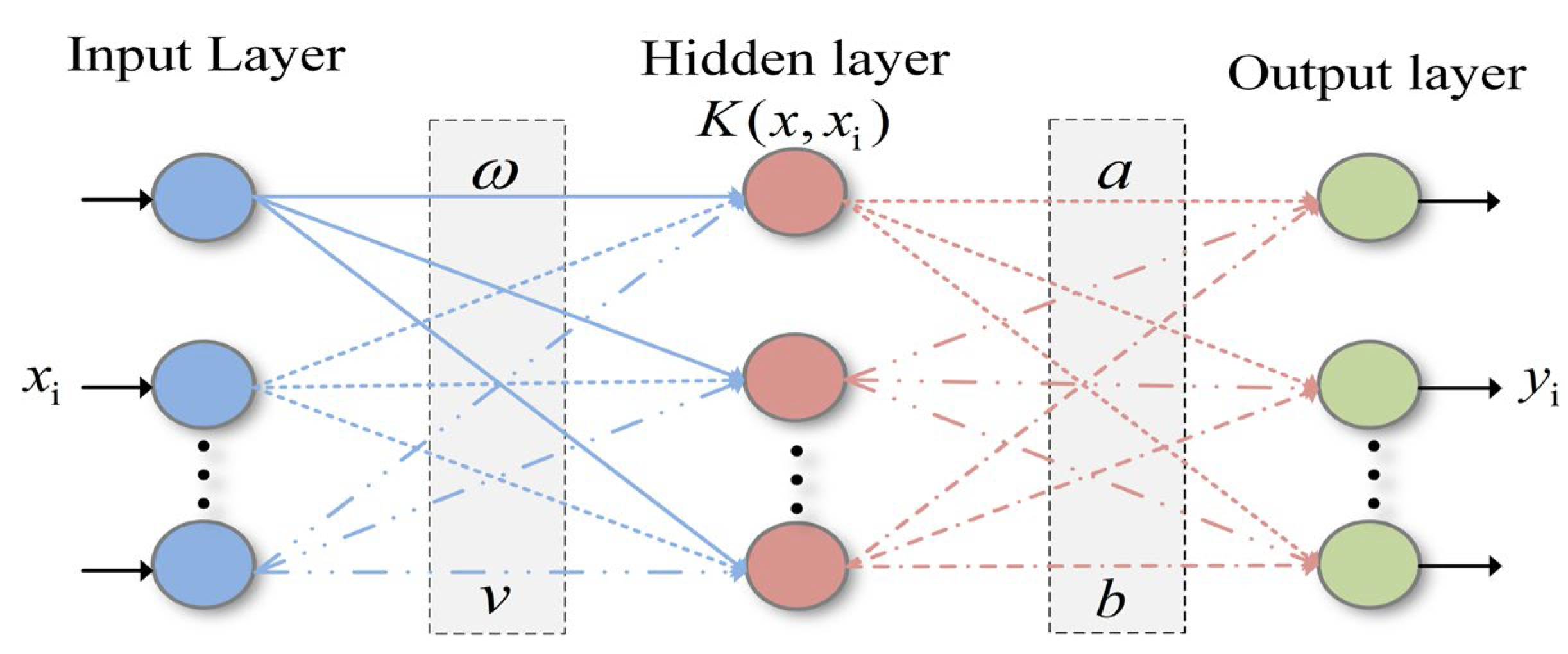
4. Kernel Extreme Learning Machine Method for PQDs Classification

4.1. Kernel Extreme Learning Machine

The KELM topology is shown in Figure 4. There are N classified training samples $(x_{\mathrm{i}},y_{\mathrm{i}})$, i = 1, 2, …, N. The output of N samples is denoted by a matrix $Y={\left[y_1,y_2,\dots ,y_{\mathrm{N}}\right]}^T$.

The KELM hidden layer neuron output is described as follows:

$$H=\left[\begin{array}{c}h(x_1)\\ ⋮\\ h(x_{\mathrm{N}})\end{array}\right]$$

(19)

The KELM optimization model is as follows:

$$\left\{\begin{array}{l}\underset{\beta }{\min }{\displaystyle \frac{1}{2}}{‖\beta ‖}^2+{\displaystyle \frac{C}{2}}{‖{\xi }_{\mathrm{i}}‖}^2\\ s.t.h(x_i)\beta =y_{\mathrm{i}}^T-{\xi }_{\mathrm{i}}^T,i=1,2,\dots ,N\end{array}\right.$$

(20)

where C is penalty coefficient, ${\xi }_{\mathrm{i}}$ is classification error. The Lagrangian expression of Equation (20) is as follows:

$$L={\displaystyle \frac{1}{2}}{‖\beta ‖}^2+{\displaystyle \frac{C}{2}}{‖{\xi }_{\mathrm{i}}‖}^2-{\displaystyle \sum _{i=1}^N{\displaystyle \sum _{j=1}^m{\alpha }_{\mathrm{i},\mathrm{j}}(h(x_{\mathrm{i}}){\beta }_{\mathrm{j}}-y_{\mathrm{i},\mathrm{j}}+{\xi }_{\mathrm{i},\mathrm{j}})}}$$

(21)

where ${\alpha }_{\mathrm{i},\mathrm{j}}$ is lagrangian multiplier. The output of KELM model can be obtained by solving the above formula, so

$$\beta =H^T{(H{H}^T+{\displaystyle \frac{I}{C}})}^{-1}Y$$

(22)

$$y=h(x)\beta =h(x)H^T{(H{H}^T+{\displaystyle \frac{I}{C}})}^{-1}Y$$

(23)

where I is the unit matrix. The kernel technique is used to map the training samples to the high-dimensional space [23,24,25]. The Mercer theorem is applied to the mapping matrix H, and the output of the KELM model can be obtained by substituting Equations (24) and (26) into Equation (23).

$$H{H}^T=h(x_{\mathrm{i}})h(x_{\mathrm{j}})=\mathrm{k}$$

(24)

$$K=K(x_{\mathrm{i}},x_{\mathrm{j}})=\left[\begin{array}{ccc}K(x_1,x_1)& \cdots & K(x_1,x_{\mathrm{N}})\\ ⋮& \ddots & ⋮\\ K(x_{\mathrm{N}},x_1)& \cdots & \mathrm{k}(x_{\mathrm{N}},x_{\mathrm{N}})\end{array}\right]$$

(25)

$$h(x)H^T=K(x,x_{\mathrm{j}})=\left[\begin{array}{c}K(x,x_1)\\ ⋮\\ K(x,x_{\mathrm{N}})\end{array}\right]$$

(26)

$$y=\left[\begin{array}{c}K(x,x_1)\\ ⋮\\ K(x,x_{\mathrm{N}})\end{array}\right]{(K+{\displaystyle \frac{I}{C}})}^{-1}Y$$

(27)

4.2. Comparison of Algorithm Classification Results

The optimal feature vector set with a dimension of 150 × 10 is used as the input of the classifier, and the overall structure of the classification is shown in Figure 5. In this paper, the first 100 × 10 data set of the optimal feature vector set of each PQD is used as the training sample set of ELM and KELM, respectively, and the last 50 × 10 data set is used as the test sample set.

The ELM selects the sigmoid function as the activation function, and the KELM selects the gaussian kernel function. The classification results of fourteen kinds of PQD by KELM in Matlab2020 environment are shown in Figure 6. From the diagram it can be seen that KELM has a high degree of discrimination for 14 PQDS, and a small number of samples for C8, C9, and C13 are not enough, but the discrimination is still considered to fully meet the expectations.

The combination of KF, UKF, ELM, and KELM is used to detect and classify the data of fourteen kinds of PQDs test samples, and the corresponding success rate is calculated quantitatively. The results are shown in

Table 4. The average success rate of combined detection-classification methods.

Label	Success Rate of Different Methods
	KF-ELM	KF-KELM	UFK-ELM	UKF-KELM
C1	97	95	96	95
C2	95	96	94	98
C3	96	99	100	100
C4	98	97	99	96
C5	100	98	96	98
C6	95	100	100	100
C7	98	100	98	100
C8	100	99	96	99
C9	95	98	100	98
C10	97	100	97	96
C11	98	97	96	98
C12	100	96	100	100
C13	99	98	96	97
C14	97	100	100	99
Average rate	97.5	98.07	97.71	98.14

. The table records the success rate of KF-ELM, KF-KELM, UKF-ELM, and UKF-KELM in various cases from C1 to C14. Finally, it is concluded that the highest success rate is UKF-KELM. KELM replaces the randomly initialized weight matrix in ELM with an orthogonal matrix, which can better maintain the information of input data and improve the accuracy of classification. Table 4 shows that the success rate of the UKF-KELM detection-classification method is higher than that of other combination methods, and the average success rate of classification is 98.14%.

In order to further verify the anti-noise performance of the combined detection classification method, the detection and recognition results of voltage swell disturbance in different signal-to-noise ratio environments are shown in Figure 7. It can be seen from the figure that as the signal-to-noise ratio gradually increases, the signal interference and instability become lower, and the overall success rate of voltage swell disturbance identification becomes higher. At the same time, the four combined detection and identification methods are higher in different noise environments. The recognition success rate and anti-noise performance of UKF-KELM are better.

The comparison of training and testing times between UKF-ELM and UKF-KELM for recognition and classification is shown in

Table 5. Algorithm training time.

	UKF-ELM	UKF-KELM
Training time/s	0.0015	0.0026
Test time/s	0.0018	0.0401

. As indicated by the table, although the UKF-KELM achieves superior accuracy and performance, its training and testing times remain similar to those of the UKF-ELM, without any significant increase. UKF-KELM enhances nonlinear modeling capability by incorporating kernel techniques, but its computational complexity does not differ significantly from UKF-ELM, as both models’ computational bottleneck mainly lies in the Kalman filter process. Nonetheless, UKF-KELM performs better in handling complex power quality disturbances, offering higher classification accuracy. Its limitation primarily lies in the sensitivity to kernel function selection, where an inappropriate kernel may lead to degraded performance.

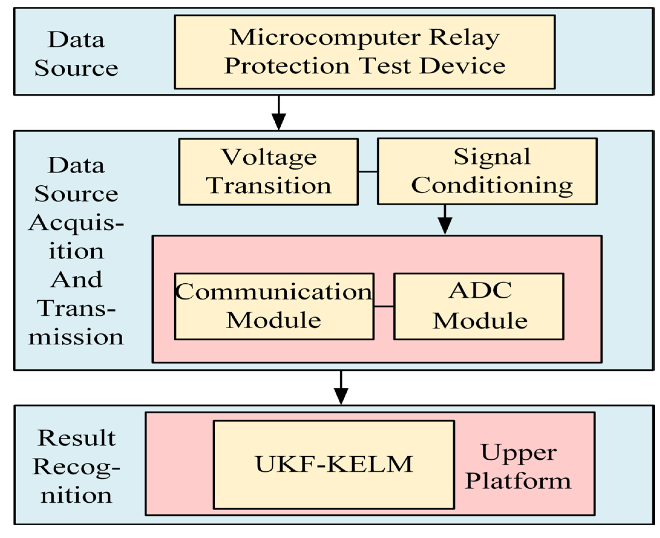
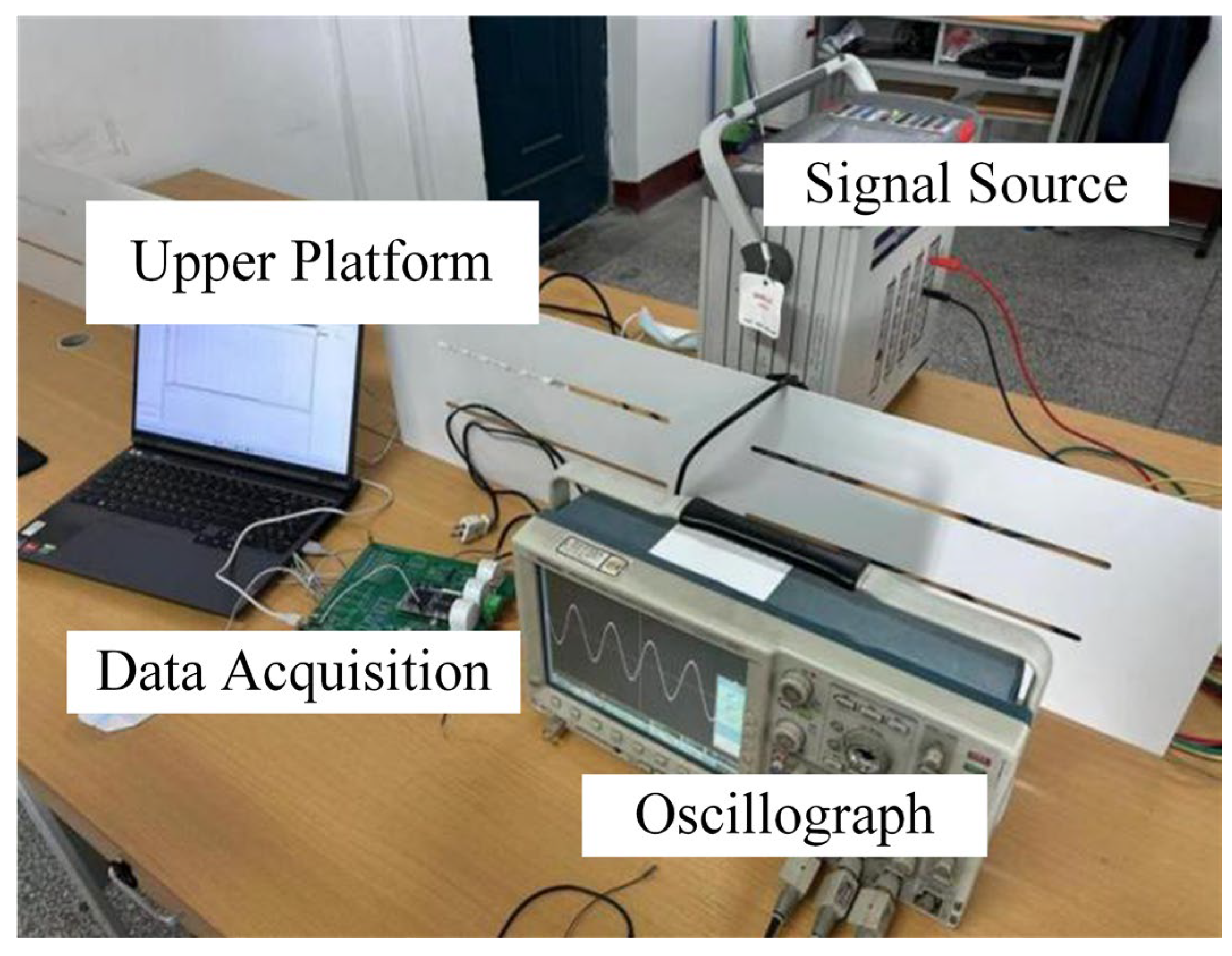
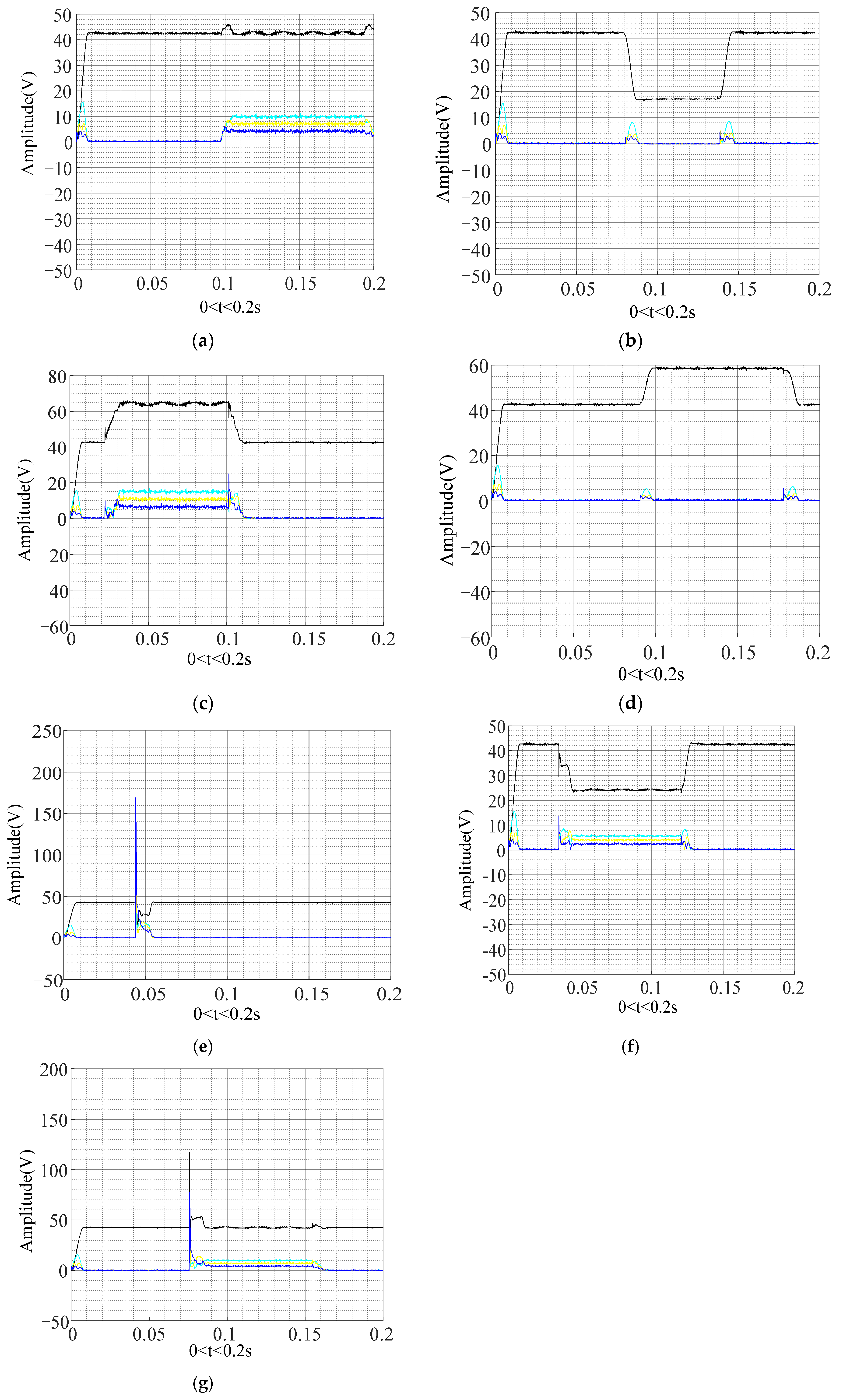
5. Experimental Verification

In order to further verify the effectiveness of the PQDs classification method proposed in this paper, an experimental platform for PQDs detection and classification is built. The overall scheme is shown in Figure 8. The experimental platform is built as shown in Figure 9. The experimental equipment table is shown in

Table 6. The experimental equipment table.

Experiment Equipment	Number	Equipment Type
Upper Platform	1	Matlab2020
Data Acquisition	1	STM32H743IIT6
Oscillograph	1	-
Microcomputer relay protection test device	1	ONLLY-AD461

. The microcomputer relay protection test device is used to simulate the disturbance source to generate the disturbance signal, and the three-phase voltage is processed by the signal acquisition circuit to obtain the disturbances that conform to the chip voltage. The UKF-KELM classification method is applied to the hardware platform to classify the disturbances. The experimental part analyzes seven kinds of disturbances, such as voltage swell, voltage sag, voltage pulse, harmonics, harmonics + swell, harmonics + sag, and harmonics + pulse. The effective value of the output normal voltage is set to 30 V, and the frequency is 50 Hz.

UKF is used to track and detect the amplitudes of the fundamental wave, third harmonic, fifth harmonic, and seventh harmonic in real time. The hardware platform detects seven kinds of disturbance results, as shown in Figure 10. In the figure, the black curve represents the fundamental wave, the bright blue curve represents the third harmonic, the yellow curve represents the fifth harmonic, and the blue curve represents the seventh harmonic. The disturbance type in Figure 10a is the harmonics. UKF tracks and detects the third harmonic, the fifth harmonic, and the seventh harmonic, and the disturbance amplitude is stable near 10 V, 7 V, and 4 V, respectively. The disturbance type in Figure 10b is voltage sag, which does not contain harmonics, and the minimum voltage drops to around 17 V. The type of disturbance in Figure 10c is harmonics + swell, including third, fifth, and seventh harmonics. When harmonics occur, the amplitudes are stable near 15 V, 11 V, and 7 V, respectively, and the maximum fundamental voltage is up to 65 V. The disturbance type in Figure 10d is voltage swell, which does not contain harmonics, and the maximum voltage reaches around 59 V. The disturbance type in Figure 10e is pulse, without harmonics, and the maximum voltage impact value reaches about 170 V. The disturbance type of Figure 10f is harmonics + sag, including third, fifth, and seventh harmonics. When harmonics occur, the amplitudes are stable near 6 V, 4 V, and 2 V, respectively, and the minimum value of fundamental voltage drops to near 24 V. The disturbance type of Figure 10g is harmonics + pulse, including third, fifth, and seventh harmonics. When harmonics occur, the amplitudes are stable near 10 V, 6 V, and 4 V, respectively, and the fundamental voltage impulse value is near 120 V.

The success rate of hardware platform classification is shown in

Table 7. Success rate of hardware platform classification.

Label	UKF-KELM/%
C1	97
C2	98
C5	97
C7	100
C1 + C7	96
C2 + C7	100
C5 + C7	98
Average rate	98.00

. It can be seen from the table that the accuracy of UKF-KELM is very high when judging a single disturbance type, and it still maintains high accuracy in the face of complex multi-disturbance situations. The average success rate of UKF-KELM classification is 98%, which verifies the effectiveness of the PQDs classification method proposed in this paper.

6. Conclusions

In this paper, a novel algorithm for PQD classification based on UKF and KELM is proposed. The UKF is used to detect and process the original disturbances, and the performance of the signal detection methods is compared by analyzing the indices of both KF and UKF in tracking and detecting voltage swell disturbances. The results show that UKF outperforms KF, providing better robustness against interference and noise. For feature extraction, real-time tracking of the amplitudes of the fundamental wave, third harmonic, fifth harmonic, seventh harmonic, and oscillatory wave is performed, with the minimum and peak indices being selected as the optimal feature vector set. The combination of KF, UKF, ELM, and KELM is applied to classify fourteen types of PQDs in simulation, achieving an average classification success rate of 98.14%. The experimental results further demonstrate the method’s effectiveness and feasibility, with an average classification success rate of 98%.

Future work will focus on optimizing the UKF-KELM algorithm to handle more complex disturbances and improve its real-time performance. Expanding the classification to cover more PQD types and exploring multi-modal data fusion are also potential directions. Additionally, the real-time implementation of the proposed method in industrial PQD monitoring systems will be investigated to assess its scalability and practical application.

References

1. Wang, L.Q.; Jin, Y.; Li, H.X.; Li, Y.; Li, Y.C.; Zhang, K.J.; Liu, H.; Cheng, L. An advanced quantum support vector machine for power quality disturbance detection and identification. EPJ Quantum Technol. 2024, 11, 70. [Google Scholar] [CrossRef]
2. Wang, J.; Xu, Z.; Che, Y. Power Quality Disturbance Classification Based on DWT and Multilayer Perceptron Extreme Learning Machine. Appl. Sci. 2019, 9, 2315. [Google Scholar] [CrossRef]
3. Lin, W.-M.; Wu, C.-H. Fast Support Vector Machine for Power Quality Disturbance Classification. Appl. Sci. 2022, 12, 11649. [Google Scholar] [CrossRef]
4. Rao, X.J.; Zhou, K.; Wang, X.J.; Li, M.Z.; Huang, Y.L.; Xie, M. Suppression of narrow-band noise of partial discharge based on improved SVD algorithm. High Volt. Eng. 2021, 47, 705–713. [Google Scholar]
5. Cheng, J.; Zhang, Z.; Yan, R.; Li, X.; Xie, Z.; Hu, Z. Transient power quality disturbance localization and detection method based on SVD-ILMD. Zhejiang Electr. Power 2024, 43, 1–11. [Google Scholar]
6. Huang, J.; Li, X. Detection of harmonic in power system based on short-time Fourier transform and spectral kurtosis. Power Syst. Prot. Control 2017, 45, 43–50. [Google Scholar]
7. Chen, Z.; Wang, L.; Yi, Y. Computation of radio interference excitation current of DC corona based on short-time Fourier transform. High Volt. Eng. 2019, 45, 1866–1872. [Google Scholar]
8. Jia, R.; Zhao, J.; Wu, H.; Ma, X.; Dang, J. Application of correlated probabilistic wavelet transform in partial discharge detection. High Volt. Eng. 2017, 43, 2896–2902. [Google Scholar]
9. Khetarpal, P.; Nagpal, N.; Alhelou, H.H.; Siano, P.; Al-Numay, M. Noisy and non-stationary power quality disturbance classification based on adaptive segmentation empirical wavelet transform and support vector machine. Comput. Electr. Eng. 2024, 118, 109346. [Google Scholar] [CrossRef]
10. Ke, Z.; Qingren, J.; Zhiyue, M. Power quality disturbance detection based on partitioning-improved empirical wavelet transform. J. Phys. Conf. Ser. 2023, 2659, 012023. [Google Scholar]
11. Cui, Y.; Xi, Y.; Zhang, X. Detection of harmonic based on residual analysis using adaptive Kalman filter. Power Syst. Prot. Control 2019, 47, 92–100. [Google Scholar]
12. Xu, H.; Guo, G.; Yu, L.; Qin, F.; Chen, J. Nonnegative definite adaptive Kalman filter based detection. Sci. Technol. Eng. 2020, 20, 3611–3616. [Google Scholar]
13. Liu, Y.; Wu, Z.; Li, T.; Han, W.; Fang, M. Implementation of Power Quality Detection Technology Based on Kalman Filtering Algorithm. Autom. Instrum. 2023, 7, 294–298. [Google Scholar]
14. Rodriguez, M.A.; Sotomonte, J.F.; Cifuentes, J.; Bueno-López, M. A classification method for power-quality disturbances using Hilbert–Huang transform and LSTM recurrent neural networks. J. Electr. Eng. Technol. 2021, 16, 249–266. [Google Scholar] [CrossRef]
15. Wang, J.; Xu, Z.; Che, Y. Power quality disturbance classification based on compressed sensing and deep convolution neural networks. IEEE Access 2019, 7, 78336–78346. [Google Scholar] [CrossRef]
16. Cai, K.; Hu, T.; Cao, W.; Li, G. Classifying power quality disturbances based on phase space reconstruction and a convolutional neural network. Appl. Sci. 2019, 9, 3681. [Google Scholar] [CrossRef]
17. Qu, H.; Liu, H.; Li, X.; Huang, J. Recognition of multiple power quality disturbances using multi-label random forest. Power Syst. Prot. Control. 2017, 45, 1–7. [Google Scholar]
18. Chen, H.; Yu, Z. Overview of power quality analysis. China Insp. Body Lab. 2022, 30, 11–14. [Google Scholar]
19. Samanta, S.I.; Mohanty, S.; Parida, M.S.; Rout, P.K.; Panda, S.; Bajaj, M.; Blazek, V.; Prokop, L.; Misak, S. Artificial intelligence and machine learning techniques for power quality event classification: A focused review and future insights. Results Eng. 2025, 25, 103873. [Google Scholar] [CrossRef]
20. Indragandhi, V.; Kumar, S.R.; Saranya, R. Hilbert-Huang Transform and machine learning based electromechanical analysis of induction machine under power quality disturbances. Results Eng. 2024, 24, 103075. [Google Scholar] [CrossRef]
21. He, H.; Xin, Z.; Wang, L.; Tan, F.; Kong, C. Detection method of power quality disturbance based on feature vector selection and double-layer BPNN. High Volt. Eng. 2022, 48, 1237–1250. [Google Scholar]
22. Cheng, X.; Wang, A.; Hua, R.; Meng, G. Research on the performance of 24 feature indicators for bearing state recognition. J. Vib. Meas. Diagn. 2016, 36, 351–358. [Google Scholar]
23. Li, C.; Xu, M. Concept, properties, and construction methods of kernel functions. Comput. Knowl. Technol. 2015, 11, 171–173. [Google Scholar]
24. Wu, S.; Jiang, J.; Yan, Y.; Bao, W. Short-term load forecasting based on VMD-PSO-MKELM method. Proc. Chin. Soc. Univ. Electr. Autom. Electr. Power Syst. 2022, 34, 18–25. [Google Scholar]
25. Yi, H.; Gao, Y.; Zhu, Y.; Huang, R.; Huang, C. Recognition of composite power quality disturbance based on improved incomplete S transform and LOO-KELM algorithm. Electr. Power Autom. Equip. 2022, 42, 199–205. [Google Scholar]
Figure 1. The flowchart of UKF algorithm.
Applsci 15 02721 g001
Figure 2. Tracking voltage surge disturbance by UKF. (a) In total, 40 db amplitude variation; (b) 20 db amplitude variation.
Applsci 15 02721 g002
Figure 3. The index distribution of different feature quantities with single disturbance. (a) Minimum feature distribution; (b) peak index characteristic distribution.
Applsci 15 02721 g003
Figure 4. KELM topological structure.
Applsci 15 02721 g004
Figure 5. The structure diagram of KELM to identify PQDs.
Applsci 15 02721 g005
Figure 6. The classification results of fourteen kinds of PQDs by KELM.
Applsci 15 02721 g006
Figure 7. The success rate of voltage swell detection and recognition in different noise environments.
Applsci 15 02721 g007
Figure 8. The overall scheme of PQDs classification system.
Applsci 15 02721 g008
Figure 9. The experimental platform of PQDs classification system.
Applsci 15 02721 g009
Figure 10. The test results of the hardware platform. (a) Harmonic disturbance; (b) voltage sag; (c) harmonics and voltage swell; (d) voltage swell; (e) voltage pulse; (f) harmonics and voltage sag; (g) harmonics and voltage pulse.
Applsci 15 02721 g010