
Magnetic Moment Estimation Algorithm Based on Convolutional Neural Network

 and
and
Abstract
1. Introduction
2. Materials and Methods
2.1. Magnetic Anomaly Detection
2.1.1. Principles and Methods
2.1.2. Geomagnetic Field, Magnetic Moment, and Magnetic Anomaly Signals
2.2. Magnetic Dipole Model
3. Model and Experiment
3.1. Neural Network Model
3.2. Dataset
- 1.
- The magnitude of the geomagnetic field is 50,000 nT, with a geomagnetic field inclination of and a declination of ;
- 2.
- The simulation range is , with a spatial sampling rate of 0.1 sampling points per meter;
- 3.
- The height varies from 500 m to 1000 m in 100 m steps;
- 4.
- The target magnetic moment modulus ranges from to A·m2, with a step size of A·m2;
- 5.
- The target magnetic moment declination ranges from to , with a step size of . The magnetic moment inclination ranges from to , with a step size of .
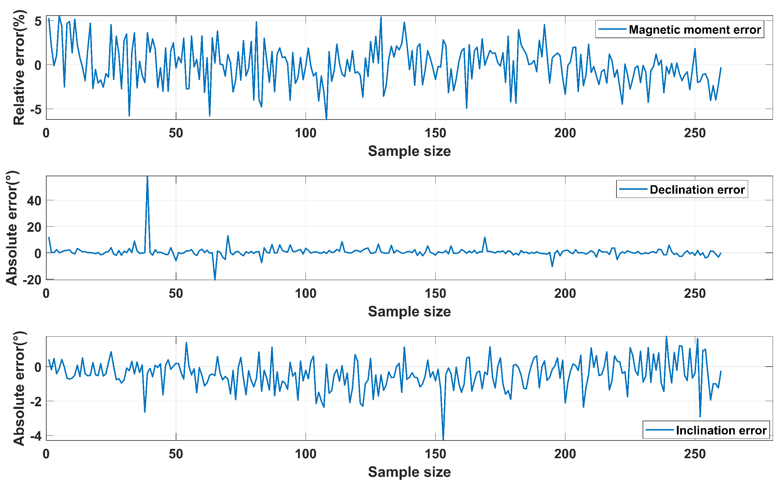
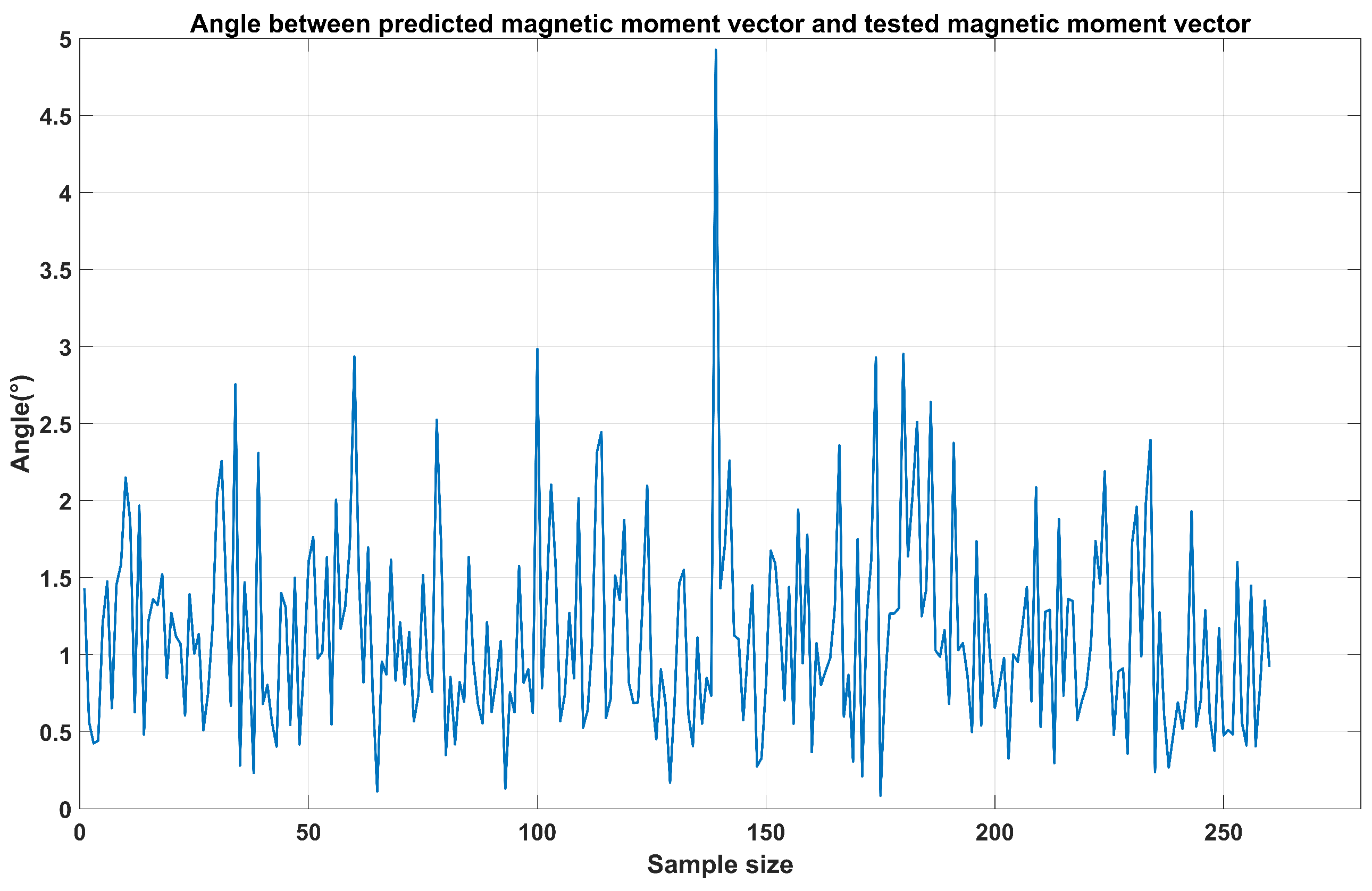
3.3. Performance Indicators
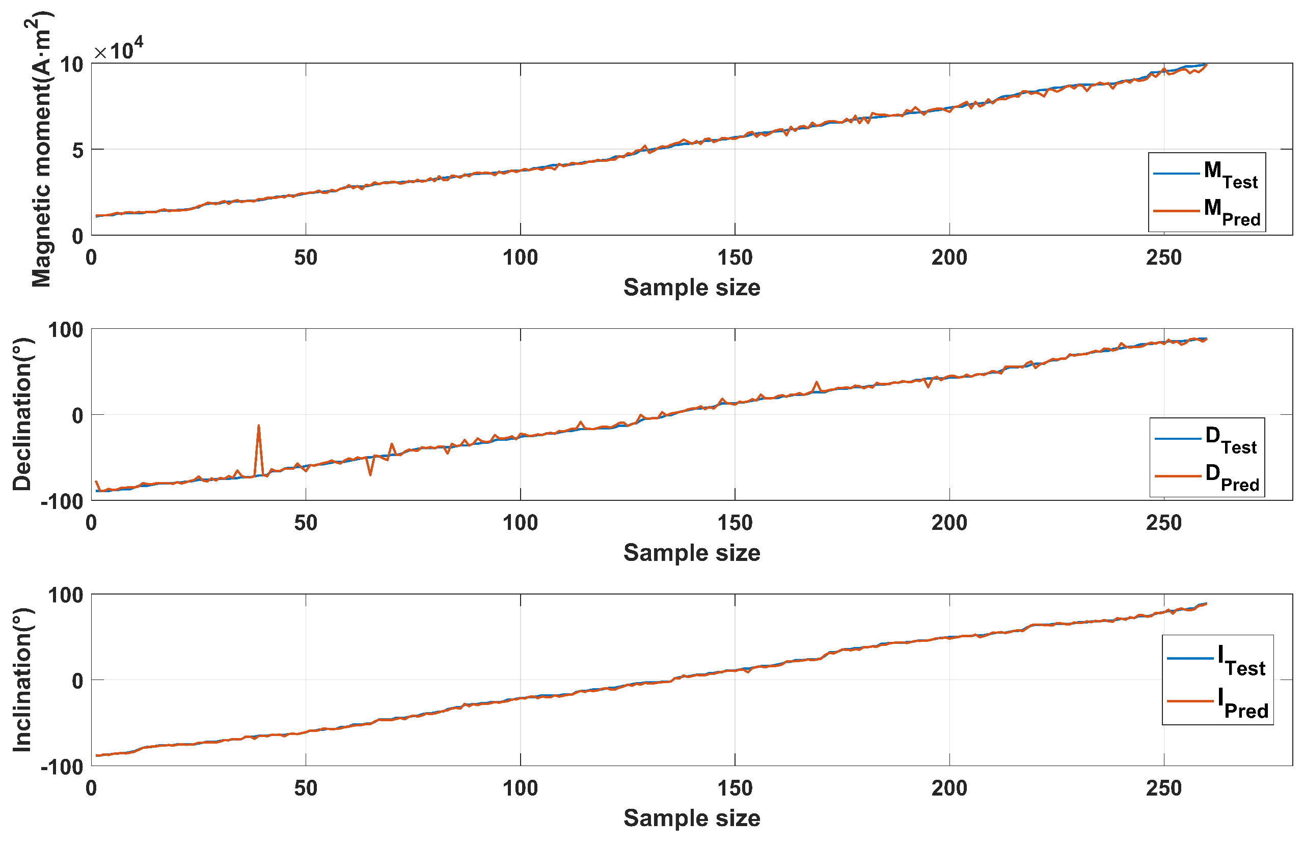
4. Results
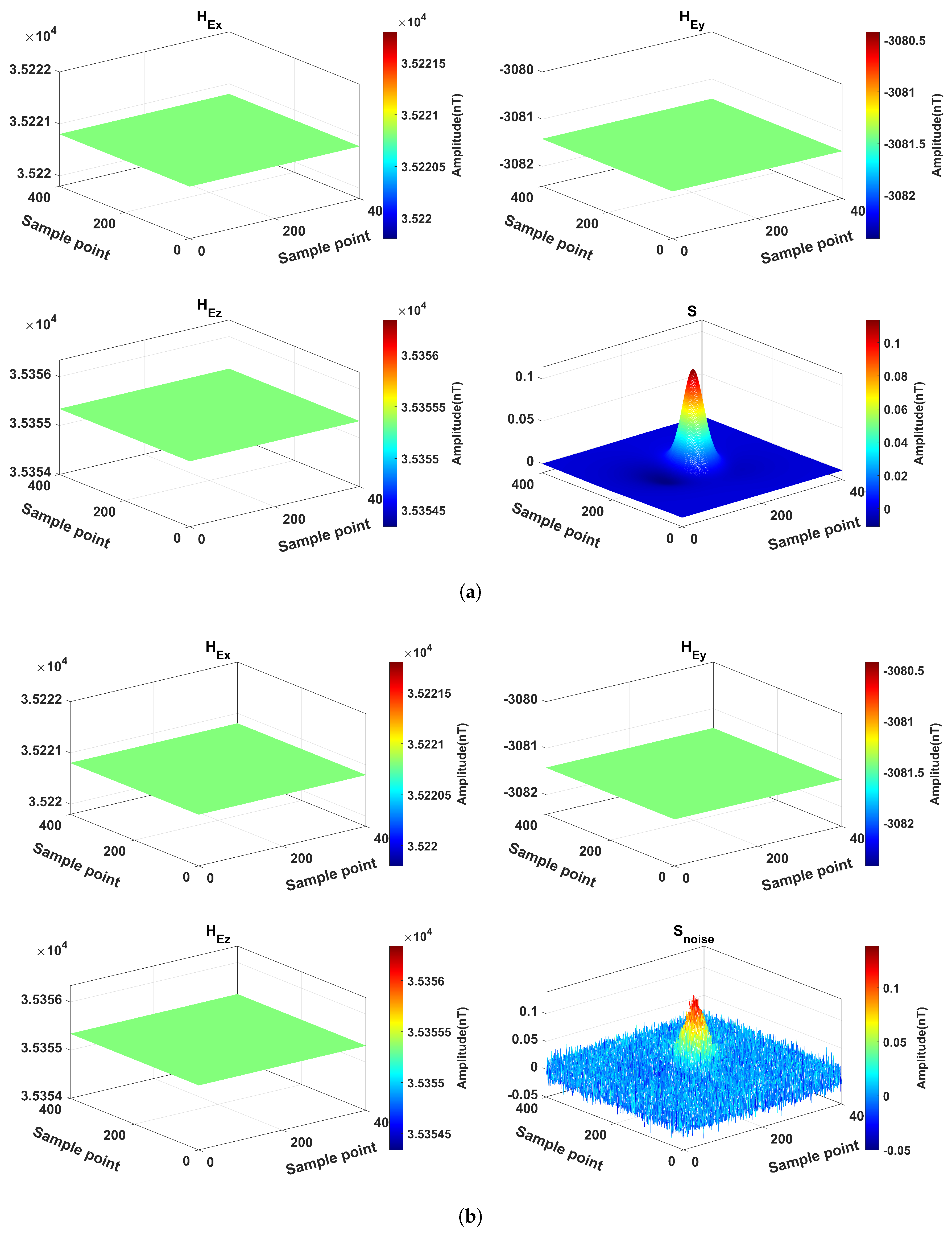
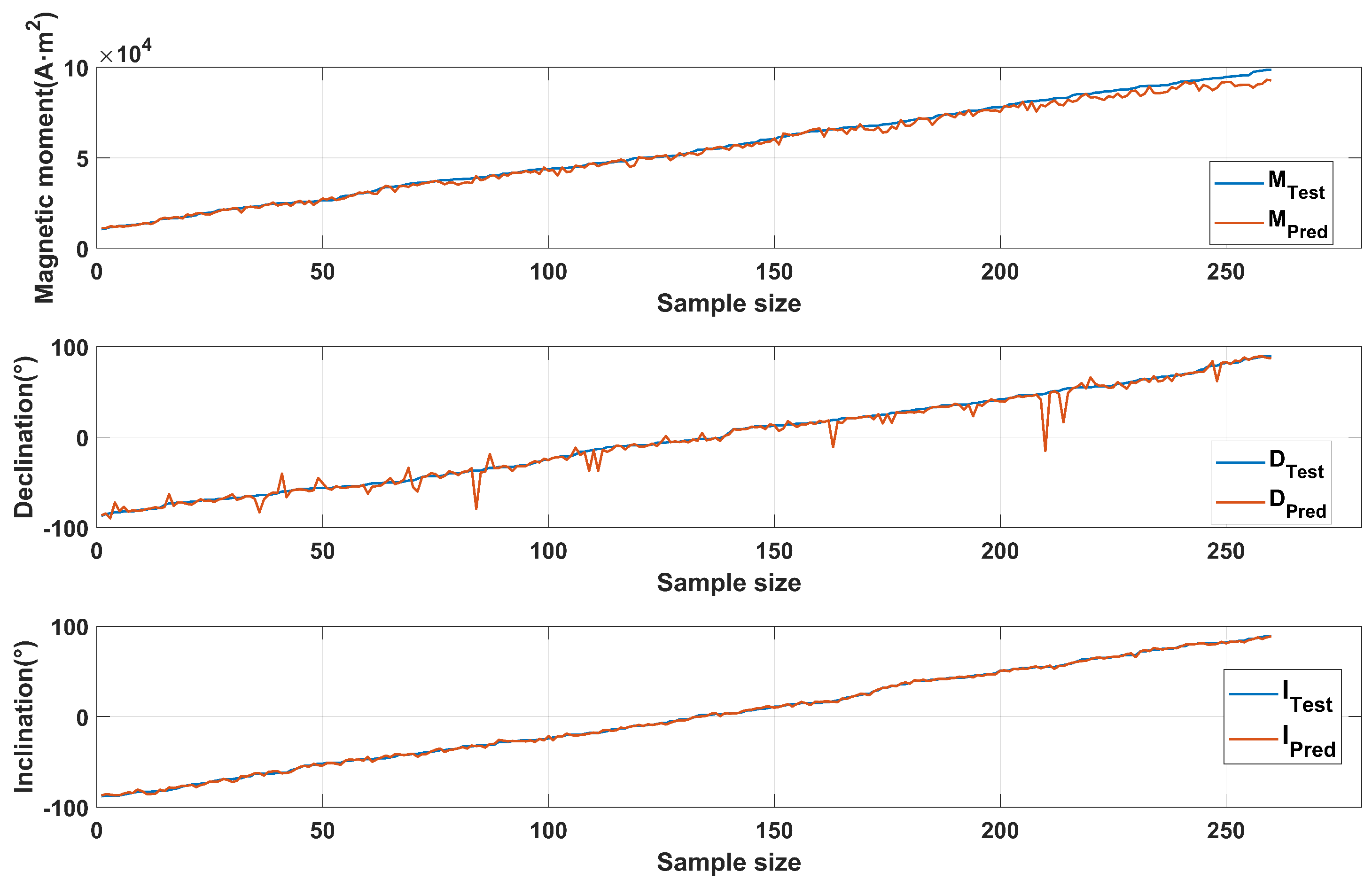
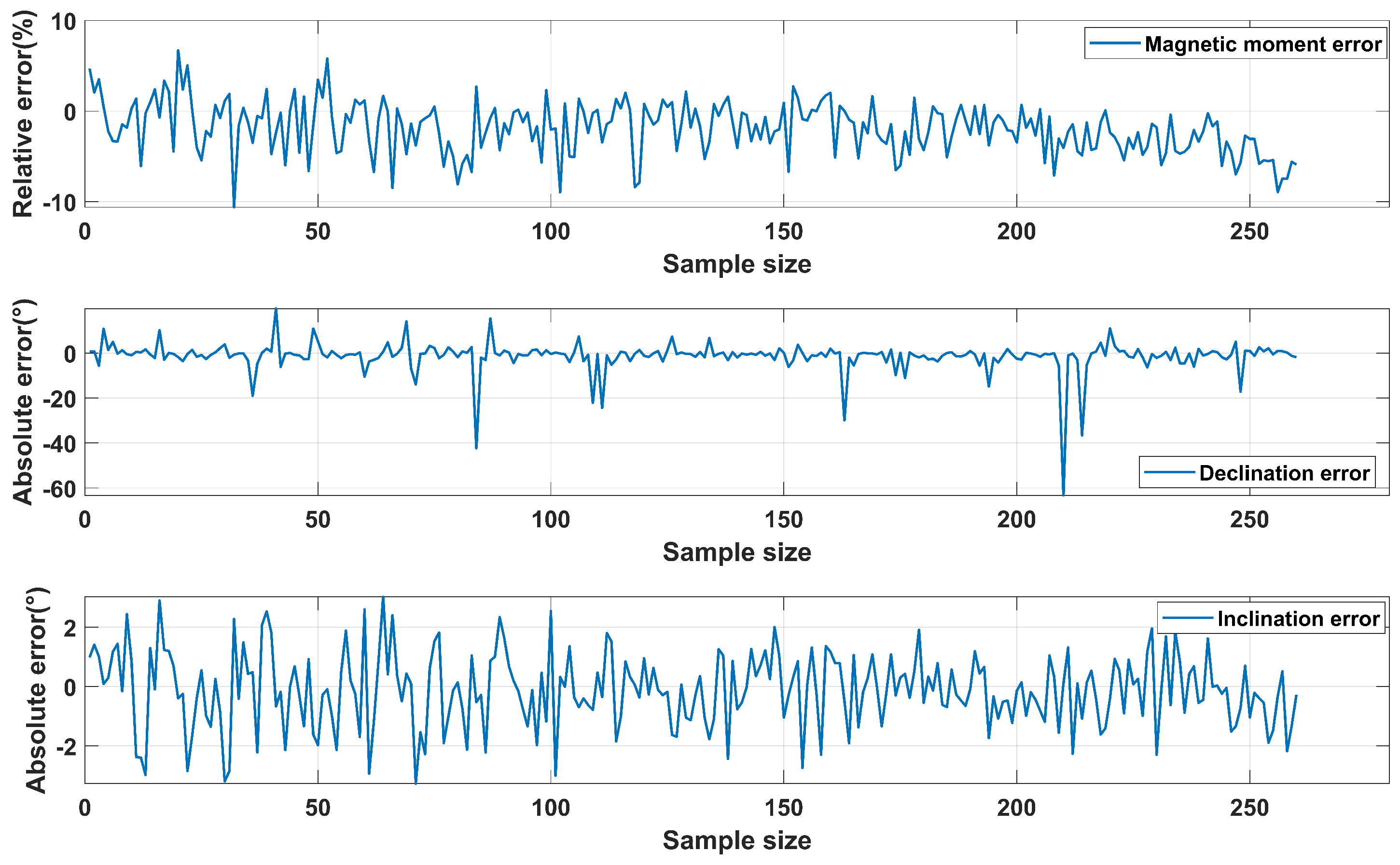
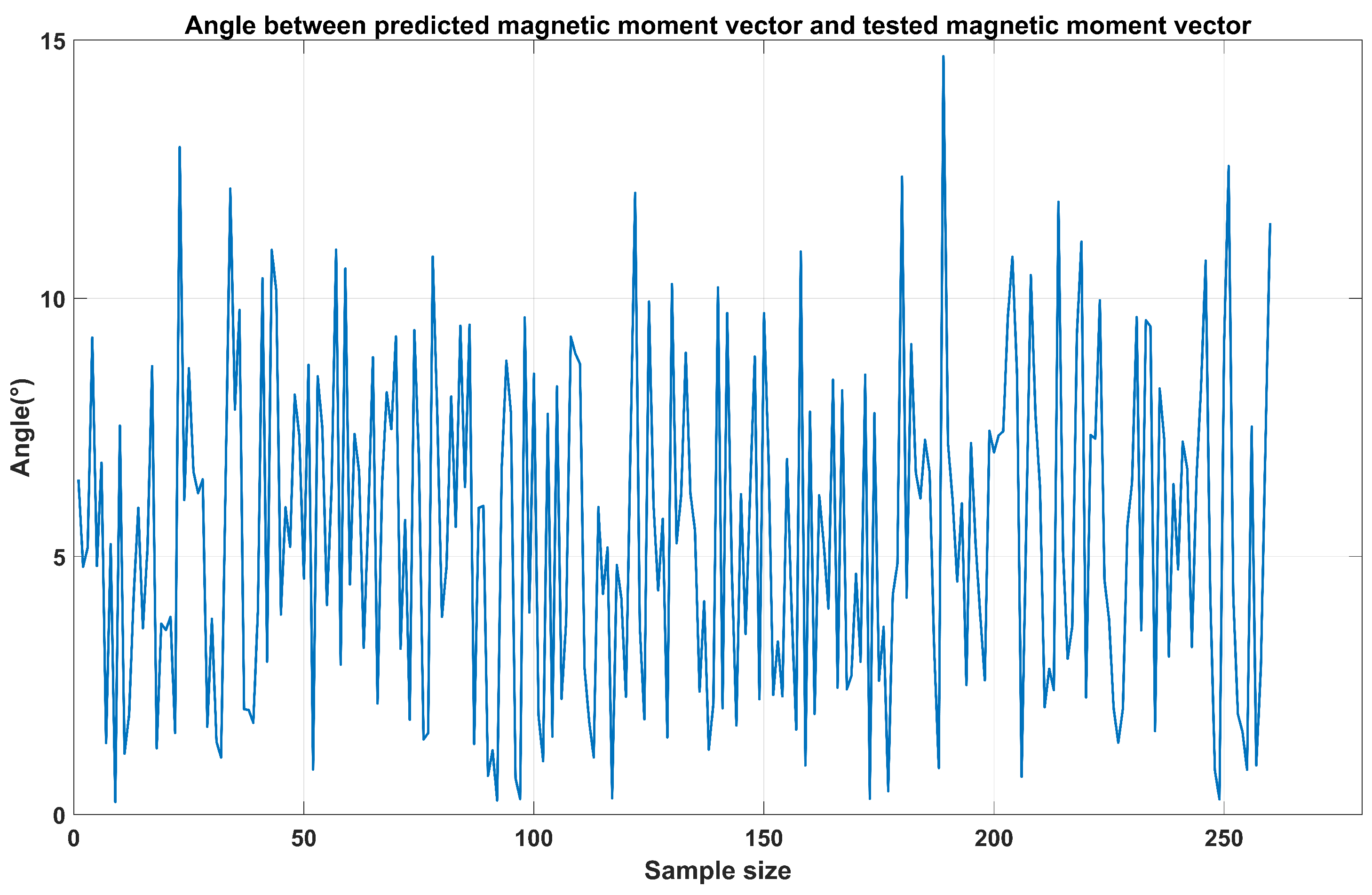
4.1. Ideal State
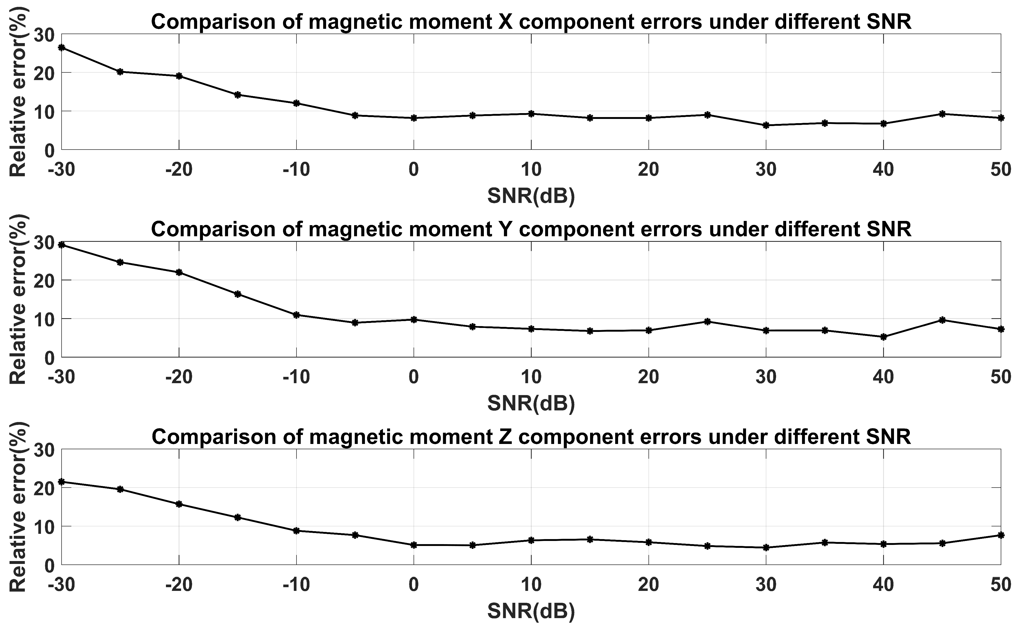
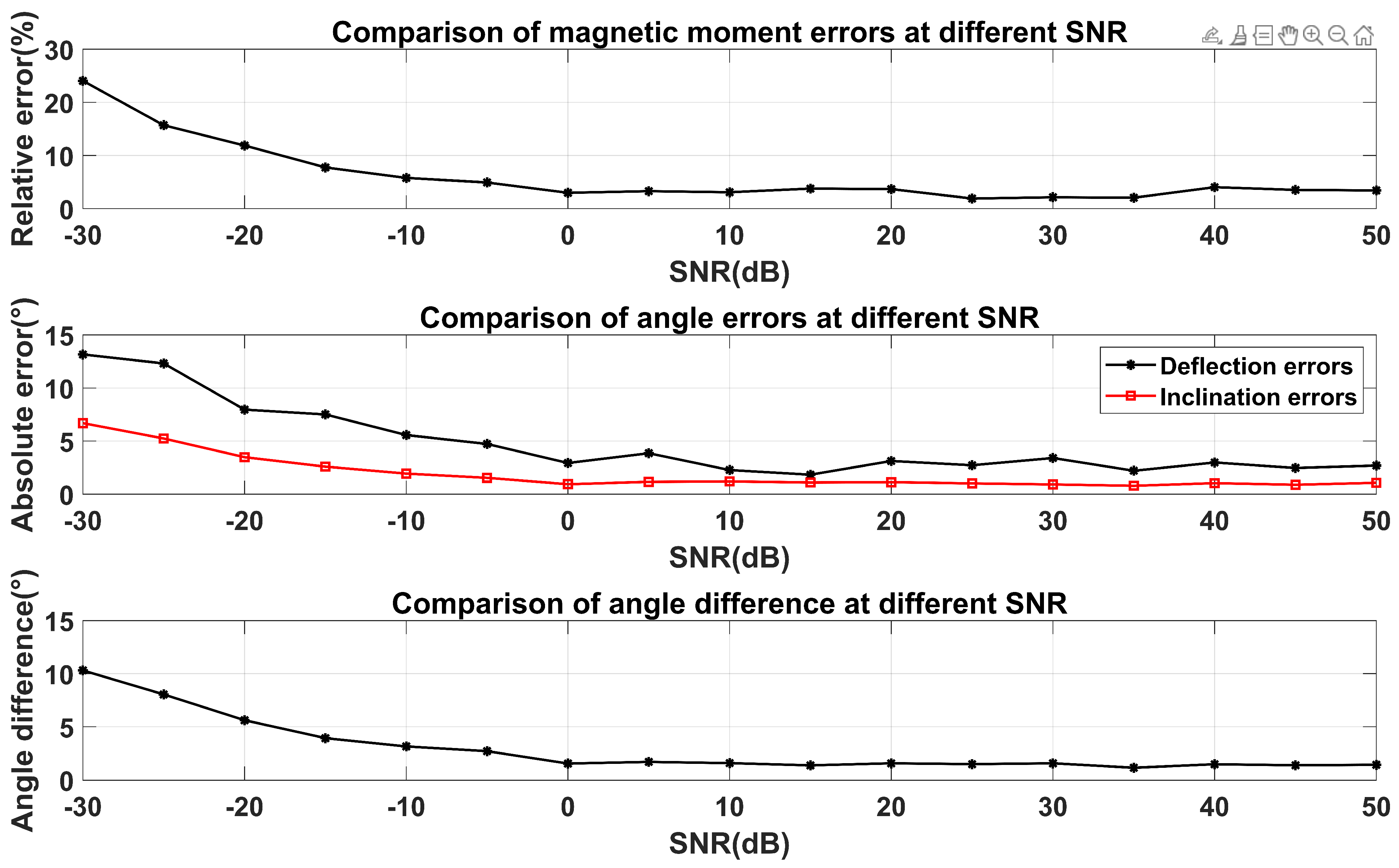
4.2. Adding Noise
5. Discussion
6. Conclusions
Author Contributions
Funding
Data Availability Statement
Acknowledgments
Conflicts of Interest
Abbreviations
| STAR | Scalar Triangulation and Ranging |
| CNN | Convolutional neural network |
| SNR | Signal-to-noise ratio |
| MAPE | Mean absolute percentage error |
| MAE | Mean absolute error |
References
- Lenz, J.E. A review of magnetic sensors. Proc. IEEE 1990, 78, 973–989. [Google Scholar] [CrossRef]
- Hood, P. History of aeromagnetic surveying in Canada. Lead. Edge 2007, 26, 1384–1392. [Google Scholar] [CrossRef]
- Gunn, P.; Dentith, M. Magnetic responses associated with mineral deposits. AGSO J. Aust. Geol. Geophys. 1997, 17, 145–158. [Google Scholar]
- Polvani, D. Current and future underwater magnetic sensing. In Proceedings of the OCEANS 81, Boston, MA, USA, 16–18 September 1981; IEEE: Piscataway, NJ, USA, 1981; pp. 442–446. [Google Scholar]
- Deng, P.; Lin, C.-s.; Zhang, J.; Tan, B. Adaptive detection of magnetic target in aeromagnetic survey. In Proceedings of the 2010 3rd International Conference on Computer Science and Information Technology, Chengdu, China, 9–11 July 2010; IEEE: Piscataway, NJ, USA, 2010; Volume 2, pp. 497–501. [Google Scholar]
- Yin, G.; Zhang, Y.; Fan, H.; Li, Z.; Ren, G. Detection, localization and classification of multiple dipole-like magnetic sources using magnetic gradient tensor data. J. Appl. Geophys. 2016, 128, 131–139. [Google Scholar]
- Billings, S.D.; Herrmann, F.J. Automatic detection of position and depth of potential UXO using continuous wavelet transforms. In Detection and Remediation Technologies for Mines and Minelike Targets VIII; SPIE: Bellingham, WA, USA, 2003; Volume 5089, pp. 1012–1022. [Google Scholar]
- Wang, J.; Shen, Y.; Zhao, R.; Zhou, C.; Gao, J. Estimation of dipole magnetic moment orientation based on magnetic signature waveform analysis by a magnetic sensor. J. Magn. Magn. Mater. 2020, 505, 166761. [Google Scholar] [CrossRef]
- Mersch, E.; Yvinec, Y.; Dupont, Y.; Neyt, X.; Druyts, P. Underwater magnetic target localization and characterization using a three-axis gradiometer. In Proceedings of the OCEANS 2014-TAIPEI, Taipei, Taiwan, 7–10 April 2014; IEEE: Piscataway, NJ, USA, 2014; pp. 1–6. [Google Scholar]
- Billings, S.D. Discrimination and classification of buried unexploded ordnance using magnetometry. IEEE Trans. Geosci. Remote Sens. 2004, 42, 1241–1251. [Google Scholar] [CrossRef]
- Wynn, W.; Frahm, C.; Carroll, P.; Clark, R.; Wellhoner, J.; Wynn, M. Advanced superconducting gradiometer/magnetometer arrays and a novel signal processing technique. IEEE Trans. Magn. 1975, 11, 701–707. [Google Scholar] [CrossRef]
- Wiegert, R. Magnetic STAR technology for real-time localization and classification of unexploded ordnance and buried mines. In Detection and Sensing of Mines, Explosive Objects, and Obscured Targets XIV; SPIE: Bellingham, WA, USA, 2009; Volume 7303, pp. 514–522. [Google Scholar]
- Liu, J.; Li, X.; Zeng, X. A real-time magnetic dipole localization method based on cube magnetometer array. IEEE Trans. Magn. 2019, 55, 4003609. [Google Scholar] [CrossRef]
- Sheinker, A.; Lerner, B.; Salomonski, N.; Ginzburg, B.; Frumkis, L.; Kaplan, B.Z. Localization and magnetic moment estimation of a ferromagnetic target by simulated annealing. Meas. Sci. Technol. 2007, 18, 3451. [Google Scholar] [CrossRef]
- Ege, Y.; Sensoy, M.G.; Kalender, O.; Nazlibilek, S. Numerical analysis for remote identification of materials with magnetic characteristics. IEEE Trans. Instrum. Meas. 2011, 60, 3140–3152. [Google Scholar] [CrossRef]
- Qin, Y.; Li, M.; Li, K.; Pan, Y.; Yang, X.; Ouyang, J. Target magnetic moment orientation estimation method based on full magnetic gradient orthonormal basis function. AIP Adv. 2022, 12, 035035. [Google Scholar] [CrossRef]
- Ou, J.; Qiu, J.; Xie, D.; Wang, Z.; Du, J.; Chang, Q. Research on the moving magnetic object recognition method based on magnetic signature waveform. IEEE Trans. Magn. 2021, 58, 6500108. [Google Scholar] [CrossRef]
- Yan, H.; Xiao, C.; Liu, S.; Zhang, Z. Horizontal error calibration method for triaxial fluxgate magnetometer. In Proceedings of the 2008 World Automation Congress, Waikoloa, HI, USA, 28 September–2 October 2008; IEEE: Piscataway, NJ, USA, 2008; pp. 1–5. [Google Scholar]
- Zhang, K.; Hu, M.; Du, C.; Xia, M. Detection of magnetic dipole target signals by using convolution neural network. In Proceedings of the 2018 Cross Strait Quad-Regional Radio Science and Wireless Technology Conference (CSQRWC), Xuzhou, China, 21–24 July 2018; IEEE: Piscataway, NJ, USA, 2018; pp. 1–3. [Google Scholar]
- Fan, L.; Kang, C.; Zhang, X.; Zheng, Q.; Wang, M. An efficient method for tracking a magnetic target using scalar magnetometer array. SpringerPlus 2016, 5, 502. [Google Scholar] [CrossRef] [PubMed]
- Du, C.; Xia, M.; Huang, S.; Xu, Z.; Peng, X.; Guo, H. Detection of a moving magnetic dipole target using multiple scalar magnetometers. IEEE Geosci. Remote Sens. Lett. 2017, 14, 1166–1170. [Google Scholar] [CrossRef]
- Jin, H.; Wang, H.; Zhuang, Z.; Qian, Q.; Wu, C.; Shi, Y. Underwater target correlation detection and location method based on normalized magnetic moment. Meas. Sci. Technol. 2024, 35, 045114. [Google Scholar] [CrossRef]
- Hamoudi, M.; Quesnel, Y.; Dyment, J.; Lesur, V. Aeromagnetic and marine measurements. In Geomagnetic Observations and Models; Springer: Berlin/Heidelberg, Germany, 2011; pp. 57–103. [Google Scholar]
- Zhang, K.; You, X.; Liu, X.; Liu, J.; Zhu, W. Inversion of Target Magnetic Moments Based on Scalar Magnetic Anomaly Signals. Electronics 2023, 12, 4900. [Google Scholar] [CrossRef]
- Inaba, T.; Shima, A.; Konishi, M.; Yanagisawa, H.; Takada, J.i.; Araki, K. Magnetic dipole signal detection and localization using subspace method. Electron. Commun. Jpn. Part III Fundam. Electron. Sci. 2002, 85, 23–34. [Google Scholar] [CrossRef]
- Laoué, N.; Lepers, A.; Deletraz, L.; Faure, C. Neural Network Calibration of Airborne Magnetometers. In Proceedings of the 2023 IEEE 10th International Workshop on Metrology for AeroSpace (MetroAeroSpace), Milan, Italy, 19–21 June 2023; IEEE: Piscataway, NJ, USA, 2023; pp. 37–42. [Google Scholar]
- Liu, S.; Chen, Z.; Pan, M.; Zhang, Q.; Liu, Z.; Wang, S.; Chen, D.; Hu, J.; Pan, X.; Hu, J.; et al. Magnetic anomaly detection based on full connected neural network. IEEE Access 2019, 7, 182198–182206. [Google Scholar] [CrossRef]
- Chua, L.O. CNN: A vision of complexity. Int. J. Bifurc. Chaos 1997, 7, 2219–2425. [Google Scholar] [CrossRef]
- Alzubaidi, L.; Zhang, J.; Humaidi, A.J.; Al-Dujaili, A.; Duan, Y.; Al-Shamma, O.; Santamaría, J.; Fadhel, M.A.; Al-Amidie, M.; Farhan, L. Review of deep learning: Concepts, CNN architectures, challenges, applications, future directions. J. Big Data 2021, 8, 53. [Google Scholar] [CrossRef]
- Qin, Y.; Li, K.; Yao, C.; Wang, X.; Ouyang, J.; Yang, X. Magnetic anomaly detection using full magnetic gradient orthonormal basis function. IEEE Sens. J. 2020, 20, 12928–12940. [Google Scholar] [CrossRef]
- Abdelhamid, B.; Elkattan, M. Cancellation of dynamic ON/OFF effects in airborne magnetic survey. Sens. Imaging 2017, 18, 26. [Google Scholar] [CrossRef]
- De Myttenaere, A.; Golden, B.; Le Grand, B.; Rossi, F. Mean absolute percentage error for regression models. Neurocomputing 2016, 192, 38–48. [Google Scholar] [CrossRef]
- Billings, S.D.; Pasion, C.; Walker, S.; Beran, L. Magnetic models of unexploded ordnance. IEEE Trans. Geosci. Remote Sens. 2006, 44, 2115–2124. [Google Scholar] [CrossRef]
- Yu, C.; Xiang, X.; Lapierre, L.; Zhang, Q. Robust magnetic tracking of subsea cable by AUV in the presence of sensor noise and ocean currents. IEEE J. Ocean. Eng. 2017, 43, 311–322. [Google Scholar] [CrossRef]
- Zhou, H.; Alici, G. A novel magnetic anchoring system for wireless capsule endoscopes operating within the gastrointestinal tract. IEEE/ASME Trans. Mechatron. 2019, 24, 1106–1116. [Google Scholar] [CrossRef]


| Layer | Parameter Settings |
|---|---|
| Conv1 | Conv2D: Kernel number: 16; kernel size: ; strides: 1; padding: “same”; ReLU |
| Conv2 | Conv2D: Kernel number: 32; kernel size: ; strides: 1; padding: “same”; ReLU |
| Conv3 | Conv2D: Kernel number: 64; kernel size: ; strides: 1; padding: “same”; ReLU |
| Pool1 | MaxPooling2D: pool size: ; strides: 2; padding: “same” |
| Pool2 | MaxPooling2D: pool size: ; strides: 2; padding: “same” |
| Flatten | Flatten the input to 1D vector; ReLU |
| Parameter | Settings |
|---|---|
| Local geomagnetic field setting (Modulus, Inclination, Deflection) | |
| Target magnetic moment setting (Modulus, Inclination, Deflection) | () (Step Length: ) |
| Local size | |
| Spatial sampling rate | sampling point/m |
| Relative height | (Step Length: ) |
| Performance Metrics | Error |
|---|---|
| MAPE of magnetic moment magnitude | |
| MAE of magnetic moment deflection | |
| MAE of magnetic moment inclination | |
| MAE of the angular difference between two vectors |
Disclaimer/Publisher’s Note: The statements, opinions and data contained in all publications are solely those of the individual author(s) and contributor(s) and not of MDPI and/or the editor(s). MDPI and/or the editor(s) disclaim responsibility for any injury to people or property resulting from any ideas, methods, instructions or products referred to in the content. |
© 2025 by the authors. Licensee MDPI, Basel, Switzerland. This article is an open access article distributed under the terms and conditions of the Creative Commons Attribution (CC BY) license (https://creativecommons.org/licenses/by/4.0/).
Share and Cite
You, X.; Zhang, J.; Chen, B.; Zhang, K.; Liu, X.; Yan, B.; Zhu, W. Magnetic Moment Estimation Algorithm Based on Convolutional Neural Network. Appl. Sci. 2025, 15, 2653. https://doi.org/10.3390/app15052653
You X, Zhang J, Chen B, Zhang K, Liu X, Yan B, Zhu W. Magnetic Moment Estimation Algorithm Based on Convolutional Neural Network. Applied Sciences. 2025; 15(5):2653. https://doi.org/10.3390/app15052653
Chicago/Turabian StyleYou, Xiuzhi, Junqian Zhang, Bingyang Chen, Ke Zhang, Xiaodong Liu, Bin Yan, and Wanhua Zhu. 2025. "Magnetic Moment Estimation Algorithm Based on Convolutional Neural Network" Applied Sciences 15, no. 5: 2653. https://doi.org/10.3390/app15052653
APA StyleYou, X., Zhang, J., Chen, B., Zhang, K., Liu, X., Yan, B., & Zhu, W. (2025). Magnetic Moment Estimation Algorithm Based on Convolutional Neural Network. Applied Sciences, 15(5), 2653. https://doi.org/10.3390/app15052653