Comprehensive Evaluation of Conveyor Belt Impact Resistance Using Canonical Correlation Analysis

Abstract

The aim of the research was to comprehensively evaluate the impact resistance of conveyor belts. Initially, variables were identified that describe the input conditions of the experiment (weight of impacting material, impact height, type and strength of conveyor belt) and subsequent dependent variables that describe the result of the experiment (impact force, increase in tension force, relative amount of absorbed energy, degree of damage). For each dependent variable, its dependence on input variables was monitored through multiple regression analysis. In the next step, through canonical correlation analysis, correlations were observed between the created dummy canonical variables that are a linear combination of the original variables. Based on the results, strong relationships between new canonical variables were demonstrated. A test of significance of canonical correlation using Wilk’s lambda showed that the first to third canonical correlations were statistically significant. It turns out that in the first pair of canonical variables, the strength and type of conveyor belt are strongly negatively correlated with the increase in tension force and the relative amount of energy absorbed. In the second pair, the impact height and weight of the landing material are strongly positively correlated with the impact force.

1. Introduction

From the various possibilities of transport systems, in every branch of industry, one can find the use of belt transport (mining, construction, etc.). The performance of continuous conveyor systems based on belt conveyors depends on their reliable and trouble-free operation. The belt conveyor is the most commonly used conveyor system in coal mining.

As the basic part of the conveyor, the belt is prone to various failures such as scratches, cracks, and wear [1]. When designing, manufacturing, and operating conveyor belts, we are guided by the requirements of safety, economy, and long service life. Reference [1] discusses existing techniques used in industrial production and the latest theories for detecting conveyor belt defects. The most common malfunctions encountered during operation are mainly those directly related to the conveyor belt itself [2]. A sudden increase in belt tension results in failure of the belt and damage to its structure [3]. Analysis of conveyor belt failures is carried out using a wide range of scientific methods [4]. An article [5] by authors Hu and Zong proposes a fault prediction method based on a Grey least square support vector machine, and analyzes longitudinal tearing to assess the trend of belt conveyor failure prediction. The longitudinal tearing of the conveyor belt is the topic of an article [6] by authors Li and Miao. In it, they provide an online method of detecting longitudinal tears of a conveyor and propose tracking belt images based on an improved SSR algorithm. Article [7] introduces a new method of integrated binocular vision detection (IBVD) for detecting longitudinal cracks in conveyor belts.

Traditional conveyor belt monitoring focuses on catastrophic failures. Causal modelling, such as the Bayesian methodology, provides intuitive and mathematically reliable tools for understanding the complex relationships between uncertain variables and the causes of failure [8]. Fedorko [4] uses virtual reality in the process of analyzing failures in rubber textile conveyor belts.

In their work [9], the authors Li et al. created a model of prediction and assessment of the condition of the belt conveyor based on a dynamic Bayesian network. The model is created to evaluate and predict the state of the device. In the work [10] of authors Elahi et al., a data-driven approach is presented for forecasting the gradual deterioration of conveyor belt behaviour. These data are used in a forecasting model using an artificial neural network. The authors of [11] describe a developed magnetic diagnostic device designed to monitor and assess the condition of steel cord conveyor belts.

One of the main causes of damage and often end of life of conveyor belts is dynamic stress. In the paper [12], the author states that the laboratory evaluation of the service life of a conveyor belt requires the determination of several of its properties, such as tensile strength, shear strength, resistance to ageing, punctures, etc. Reference [13] presents the results of tests that enable the definition of the influence of the conveyor belt design on belt wear, especially on punctures. Results from monitoring similar properties are presented in the paper [14] by Komander et al. Article [15] presents practical approaches to the analysis of the cross-sectional profile of conveyor belt damage based on identification and understanding of belt characteristics during operation. The article [16] by the authors Honus et al. examines the analysis of the failure of the belt conveyor in relation to the place of impact where the material is located. In the paper [17], theoretical, experimental, and numerical analyses were performed to examine the effects of the impact process, observing the degree of damage to the covering layers and the carcass of the conveyor belt. Mathematical and statistical approaches to evaluating the quality of conveyor belts in terms of their puncture resistance were discussed by the authors in the work [18]. The authors of [19,20] use regression and correlation analysis to evaluate a conveyor belt in relation to its damage. Canonical correlation analysis (CCA) is a multidimensional statistical method used to study the correlation between two groups of variables. This method has wide use. For example, canonical correlation analysis was used to detect incipient faults [21], to detect bridge structure damage [22], to evaluate and assess tunnel damage potential when the ground moves [23], and to predict the damage potential of earthquake records [24]. In order to determine electricity consumption depending on various factors (climate, location, building, consumer, etc.), the author Jiang Zigili [25] used a methodology designed on the basis of canonical correlation analysis. The CCA method was used to quantify the connection between urban rail transit station demand and the surrounding land-use patterns [26], to analyze some important indicators of transport and economic systems, and to study the relations between transport and the economic development of the area [27].

Canonical correlation analysis is widely used in medicine [28], in tracking pathogenic brain disorders [29], to identify subtypes of breast cancer [30], to track the impact of digitalization on the workforce in 19 countries [31], to analyze data related to shipping and the aquatic environment of a river [32], and to establish the relationship between heavy metals in water and size-fractionated sediments [33].

The aim of this study is to comprehensively evaluate the impact resistance of conveyor belts under laboratory conditions. To evaluate the interaction between the variables describing the conditions of the experiment and the result of the experiment, multiple regression and canonical correlation analysis are used. Using a linear combination of the original variables, new (dummy) canonical variables are created, for which mutual correlation is monitored.

2. Materials and Methods

2.1. Test Equipment and Test Samples

The Institute of Industry and Transport Logistics of the Technical University of Kosice possesses a laboratory for simulating and modelling structural parts of conveyance equipment, including conveyor belts. The laboratory also includes a testing apparatus, designed and constructed by the institute, intended for the testing of conveyor belts in terms of their puncture resistance. The testing apparatus was designed based on the current requirements arising from previous research, as well as the requirements of the manufacturer of conveyor belts—Continental Matador Rubber, Puchov, Slovakia.

Experimental research was carried out on a test device (Figure 1a) that can simulate the impact of material on a conveyor belt. A detailed description of the test device is in article [34]. The impact height is limited by the height of the device and can be adjusted up to a height of 2.6 m. The weight of falling material (from 50 to 100 kg) is simulated by means of the weight of a hammer and additional ballast weights. The impactor (spherical, pyramidal) simulates the type of landing material (non-cohering or sharp-edged material). The type of conveyor belt (CB) depends on the material from which the carcass is formed (rubber textile conveyor belt, steel cord conveyor belt; Figure 2). The strength of the conveyor belt is given by the manufacturer and indicates the tensile strength of the conveyor belt (N∙mm⁻¹). The experimental test may be carried out without a support system or with a support system consisting of an assembly of two impact rollers with a smooth steel cover (Figure 1c). In general, the impact rollers support the conveyor belt and dampen the dynamic effects of the impacting material.

In the experiment, the following input parameters were set:

• The impact height varied from 1 m to 2.2 m, with a setting differential of 0.2 metres.
• The weight of the falling hammer was in the range from 50 to 90 kg with a differentiation of 10 kg.
• The impactor of the hammer had a spherical shape (Figure 1b). The drop hammer impactor was a semi-sphere shape with a diameter of 50 mm.
• Samples of conveyor belts were extracted from rubber textile or steel cord conveyor belts with strengths of 1250 N∙mm⁻¹ and 2500 N∙mm⁻¹.

In the experiment, a roller support system was used. The impact of the material was directed between the rollers (Figure 1c). The distance between the axes of the rollers was 16 cm. Each sample had dimensions of 1400 × 150 mm. A detailed description of the method of measurement and preparation of the test samples is described in [35].

The belt specimens were stretched and attached using a hydraulic device that is part of the testing equipment. On both of their ends, the specimens were attached in hydraulically controlled jaws (Figure 3). Another hydraulic device was used to stretch the specimens. The magnitude of the stretching force was determined based on the recommendations of the conveyor belt manufacturers, particularly, as 1/10 of the belt strength per millimetre of its width. Depending on the width of the tested specimens, the stretching force applied to the belts with a strength of 1250 N∙mm⁻¹ was 18,750 N, while for the belts with a strength of 2500 N∙mm⁻¹, the stretching force magnitude was 37,500 N.

Both types of belts were manufactured by applying vulcanization technology. In the case of rubber textile conveyor belts, the manufacturing process includes the application of a rubber mixture onto both sides of the textile fabric (the carcass) and into its structure on a four-roller manufacturing line.

• A P1250 rubber textile (Continental Matador Rubber, Puchov, Slovakia) conveyor belt exhibits a tensile strength of 1250 N∙mm⁻¹; it contains 4 polyamide textile plies; its top cover layer is 6 mm thick; and its bottom cover layer is 4 mm thick. The belt is 18 mm thick.
• A P2500 rubber textile (Continental Matador Rubber, Puchov, Slovakia) conveyor belt exhibits a tensile strength of 2500 N∙mm⁻¹; it contains 4 polyamide textile plies; its top cover layer is 8 mm thick; and its bottom cover layer is 4 mm thick. The belt is 22 mm thick.

As for steel cord conveyor belts, their manufacture is based on the preparation of rubber mixtures and rubber layers and includes the process of laying the individual layers on top of each other and then pressing the material while applying the hot vulcanization bonding method.

• A ST1250 steel cord (Continental Matador Rubber, Puchov, Slovakia) conveyor belt exhibits a tensile strength of 1250 N∙mm⁻¹; its top cover layer is 8 mm thick, and its bottom cover layer is 6 mm thick. The cord spacing is 13 mm and the cord diameter is 4.1 mm. The steel cord structure is (1 + 6) + 6(1 + 6). The structure of the cord core consists of 1 strand, while the whole cord structure contains 6 more strands. The steel cord is of a circular shape. The belt thickness is 18.1 mm, and its weight is 27 kg∙m⁻².
• A ST2500 steel cord (Continental Matador Rubber, Puchov, Slovakia) conveyor belt exhibits a tensile strength of 2500 N∙mm⁻¹; its top cover layer is 12 mm thick, and its bottom cover layer is 8 mm thick. The cord spacing is 15 mm and the cord diameter is 6.8 mm. The steel cord structure is 7 × 19 (7 strands; 19 wires in each strand). The belt thickness is 26.8 mm, and its weight is 41 kg∙m⁻².

Both the rubber textile and the steel cord conveyor belts have cover layers of the same category type M (intended for the transport of abrasive sharp-edged multi-piece materials). Their elongation is 450%; their abrasiveness is 120 mm³; and the Shore hardness is 60.8 Shore.

The tested conveyor belts are used in the mining industry to transport large-piece materials that are poured from a bucket-wheel excavator in the brown coal mining process. The impact height simulated the height of the chutes used in a real-life facility, while the weight of the drop hammer simulated a specific weight of coal, and the impactor type simulated the shape of the transported material (coal and accompanying rocks). The experimental parameters were chosen based on the experience gained in our previous research as well as the requirements demanded by the industry [17,18,34].

2.2. Result of Experimental Research

The result of the experiment is described by several parameters: rebound height, impact force, tension force, relative amount of absorbed energy, and degree of damage to the conveyor belt after the impact of the hammer. During the test itself, the rebound height, the amount of the tension, and the impact forces are measured using two strain gauge sensors. The measured values are recorded by PP065 electronics, which provide control of the test rig and recording of measurement results.

Rebound height

The rebound height (m) is the height to which the hammer with the impactor bounces after each rebound from the belt until this movement is dampened.

Impact and tension force

The impact force (kN) is the force exerted by the hammer impactor on the conveyor belt. The tension force (kN) is adjusted at the beginning of the measurement based on the strength of the belt sample, according to the manufacturer’s recommendations (1/10 of the belt strength per mm width). The amount of tension force s changes during the measurement when the hammer impactor comes into contact with the belt.

Relative amount of absorbed energy

Based on the rebound height after the first rebound, we observed the parameter relative amount of absorbed energy. This is determined as the relative amount of energy absorbed by the conveyor belt after the first impact of the material on the belt sample (Figure 4).

The relative amount of energy absorbed after the first impact is defined as the following ratio:

$$E_{realt}={\displaystyle \frac{E_{p1}-E_{p2}}{E_{p1}}}={\displaystyle \frac{mg{h}_1-mg{h}_2}{mg{h}_1}}={\displaystyle \frac{h_1-h_2}{h_1}},$$

(1)

where $E_{p1}$ is the potential energy of the hammer before impact (at impact height $h_1$) and $E_{p2}$ is the potential energy of the hammer after rebounding from the conveyor belt (at the rebound height $h_2$). $m$ is the weight of the hammer and $g$ is gravitational acceleration.

Degree of Damage

Determining the degree of damage consists of the visual inspection of the conveyor belt after the test. The variable damage represents the severity of damage to the composite at the point of impact of the material and describes two main categories of damage: non-serious damage and serious damage (

Table 1. Classification of the sample according to the degree of damage [37].

Damage 0	Damage 1	Damage 2	Damage 3
Non-Serious Damage		Serious Damage
No damage is visible	Visible damage to the upper or lower covering layer (cracks, punctures) without visible damage to the carcass	Visible damage to the upper or lower covering layer and visible damage to the carcass	Puncture (simultaneous complete damage to the upper covering layer, carcass, and bottom covering layer)

). A detailed classification of damage is in article [37].

Damage 0 and Damage 1 define the degree of damage that, in the case of the practical use of the conveyor belt, would not cause it to be immediately taken out of service. On the other hand, Damage 2 and Damage 3 (serious damage) are defined as damage that would cause a conveyor belt to be taken out of service. Examples of possible damage to the test specimens are shown in Figure 5.

3. Theory/Calculation

Descriptive statistics, hypothesis testing, multiple regression analysis, and canonical correlation analysis were used to analyze the results of the experiments. The evaluation is carried out using the R program. The regression and correlation analysis were carried out with the use of R version 4.4.3 and Minitab 18.1.0 software, while the canonical correlation analysis was conducted with the use of the R software (packages: CCP, CCA, ggplot, and GGally).

3.1. Statistical Inference

The basic methods of statistical inference include estimation theory and testing of statistical hypotheses. When testing statistical hypotheses, the decision to reject or accept the null hypothesis is made using the p-value. If the p-value is less than the specified significance level α, we reject the null hypothesis in favour of the alternative hypothesis. If the p-value is equal to or greater than the selected significance level α, we do not reject the null hypothesis.

3.2. Regression and Correlation Analysis

Let $Y$ be a dependent (output) variable and let $X_1,X_2,\dots ,X_k$ represent k-independent (input) variables. The relationship between the dependent variable $Y$ and k-independent variables $X_i$, $i=1,\cdots ,k$ can be written in the following form:

$$Y={\beta }_0+{\sum }_{i=1}^k{\beta }_i{X}_i+\epsilon$$

(2)

where ${\beta }_0$ and ${\beta }_i$ for $i=1,\cdots ,k$ are the parameters (coefficients) of the regression model, and ε is a random error.

The statistical significance of the regression model can be verified using the F-test of the statistical significance of the model. Statistical significance tests of the regression parameter are used to verify the statistical significance of individual parameters of the regression model. The strength of dependence of variable $Y$ on the effect of k-independent variables is expressed using the multiple coefficient of determination $R^2$. The coefficient takes values from the range 〈0; 1〉. The closer the value to 1, the closer the dependence.

In regression analysis, different units and different scales of observed variables are often used. For this reason, standardized regression coefficients ${\beta }_i^{*}$, $i=1,\cdots ,k$ are used to compare and measure the relative importance of input variables to the dependent variable. The standardized regression coefficient ${\beta }_i^{*}$ expresses how much the output variable $Y$ changes with a unit change in the standardized deviation of the independent variable $X_i$ assuming that the other input variables are constant. The higher the absolute value of the coefficient ${\beta }_i^{*}$, the stronger the effect of the independent variable [38].

3.3. Canonical Correlation Analysis

Canonical correlation analysis (CCA) is a multidimensional statistical method that aims to describe as simply and concisely as possible the dependence between two groups of original variables using linear combinations [39,40]. The method is a certain generalization of multiple regression and correlation analysis. In this method, we transform a system of mutually correlated variables into a system of new variables. The method assumes a linear dependence between variables and between groups of variables. It does not require the assumption of normality of variables.

Let the variables $X_1,X_2,X_3,{\cdots X}_k$ form the first group of variables (variable group 1), and let the variables $Y_1,Y_2,Y_3,{\cdots Y}_m$ form the second group of variables (variable group 2). The goal of CCA is to find linear combinations of original variables from each group, thereby creating new artificial variables, canonical variables (similar to the principal component analysis method). Let the new canonical variable $U$ be a linear combination of the original variables $X_1,X_2,X_3,{\cdots X}_k$ and let the canonical variable V be a linear combination of the original variables $Y_1,Y_2,Y_3,{\cdots Y}_m$. The goal of CCA is to find such pairs of canonical variables so that the dependence (correlation) between them is maximum.

Initially, the first pair of canonical variables $U_1$ and $V_1$ is found. We gradually repeat the process by searching for other pairs of canonical variables $\left(U_2,V_2\right)$ up to $\left(U_q,V_q\right)$, whereby for the pair $\left(U_h,V_h\right)$ it holds that the following occurs:

$$U_h=a_{1h}{X}_1+a_{2h}{X}_2+a_{3h}{X}_3+\cdots +a_{kh}{X}_k,$$

(3)

$$V_h=b_{1h}{Y}_1+b_{2h}{Y}_2+b_{3h}{Y}_3+\cdots +b_{mh}{Y}_m,$$

(4)

for $h=1,\cdots ,q$, where $a_h=\left\{a_{1h},a_{2h},a_{3h},\cdots ,a_{kh}\right\}$, $b_h=\left\{b_{1h},b_{2h},b_{3h},\cdots ,b_{mh}\right\}$, are canonical coefficients.

In general, the number of pairs of canonical variables is equal to the lowest number of variables in each set, i.e., $q=\mathrm{m}\mathrm{i}\mathrm{n}(k,m)$.

The intensity of dependence between a pair of canonical variables is determined using a point estimate of the canonical correlation efficient R_c.

The canonical correlation coefficient has similar properties to the Pearson correlation coefficient r. The squared of the canonical correlation coefficient R_c2 is the canonical coefficient of determination. R_c2 takes values from 0 to 1, where 0 means low correlation. The closer the value of the canonical coefficient of determination to 1, the stronger the correlation of the canonical variables.

A graphical representation of the canonical correlation analysis, in general, is in Figure 6. On the left side are the original variables $X_1,X_2,X_3,{\cdots X}_k$ (variable group 1), which form the canonical variable U; on the right side are the variables $Y_1,Y_2,Y_3,{\cdots Y}_m$ (variable group 2), which form the canonical variable V. The variable $U_1$ is a linear combination of the variables $X_1,X_2,X_3,{\cdots X}_k$ and the variable $V_1$ is a linear combination of the variables $Y_1,Y_2,Y_3,{\cdots Y}_m$. The pair $\left(U_1,V_1\right)$ represents the first pair of canonical variables, the correlation of which is determined by the canonical correlation coefficient $R_{c1}$.

To verify the statistical significance of the canonical variables, an approximate F-test is used, which is based on Wilks lambda statistics. Wilks’ lambda statistics are interpreted in exactly the opposite direction to the canonical coefficient of determination $R_{c2}$. A value near 0 means high correlation, while a value near 1 means a low correlation between canonical variables [41]. Using this test, we verify the null hypothesis that all pairs of canonical variables are uncorrelated, or $H_0:{\rho }_{c1}={\rho }_{c2}=\cdots ={\rho }_{cq}=0$, where ${\rho }_{ci}$ is the canonical correlation coefficient for the ith pair of canonical variables. By rejecting the null hypothesis, it is assumed that the first pair of canonical variables is significantly correlated, i.e., ${\rho }_{c1}\ne 0.$ In a similar manner, the significance of the correlation of other pairs of canonical variables can be verified [42]. In addition to Wilks’ lambda, other approximative F-tests, such as Pilai, Lawley–Hotelling, and Roy statistics, are also used to verify the statistically significant dependence between canonical variables, etc. [43].

Redundancy means informational or functional excess, such as a greater amount of information than necessary. Unlike the canonical coefficient of correlation, it expresses the proportion of the total variability of the first group of variables explained by the canonical variable, which arose from the linear combination of the second group of variables and vice versa. In other words, redundancy is a measure of the variance of one set of variables formed from a linear combination of another set of variables [44].

4. Results and Discussion

The experimental research was carried out in order to employ the following:

• Establish a group of variables that describe conditions and results.
• Analyze variables and the relationships between them through multiple regression and canonical correlation analyses.

4.1. Determination of Variables to Be Observed

When analyzing experimental research, variables are selected (

Table 2. Summary of variables.

Variables	Description
Experiment conditions
Weight	weight of hammer (kg), from 50 kg to 90 kg
Height	impact height (metre), from 1 m to 2.2 m
Strength	conveyor belt tensile strength (N.mm−1), values 1250 N.mm−1, 2500 N.mm−1
Type	conveyor belt type: rubber textile conveyor belt (Type = 1), steel cord conveyor belt (Type = 0), reference category: steel cord conveyor belt
The result of the experiment
Fimpact	the force exerted by the hammer impactor on the belt (kN)
ΔFtension	tension force increase (kN)
Erelat	the relative amount of absorbed energy (dimensionless number) takes values from 0 to 1
Damage	damage type: Damage = 0 (no damage); Damage = 1 (non-serious damage); Damage = 2 (serious damage without puncture)

), described by the following:

• Conditions of the experiment: Weight of hammer (Weight), fall height (Height), belt strength (Strength), type of conveyor belt (Type).
• The result of the experiment: Magnitude of the impact force (F_impakt), magnitude of the tension force increments (ΔF_tension), relative amount of absorbed energy (E_relat), and degree of damage to the conveyor belt (Damage).

In the experiment, two types of conveyor belts were used: rubber textile and steel cord conveyor belts. For the purpose of further analysis, a new variable was applied—the one that describes the type of conveyor belt (Type). It is a dummy variable with two different categories. The variables may be coded arbitrarily, but we chose codes 1 and 0 for the purpose of better understanding and interpretating the results. The coding was as follows: Type = 1 for a rubber textile conveyor belt; and Type = 0 for other types of conveyor belts (steel cord). Steel cord conveyor belts did not have their own variable (the value assigned was 0); therefore, that type of conveyor belt was regarded as the reference category.

Of the 132 research samples, 70 samples were extracted from rubber textile conveyor belts and 62 from steel cord conveyor belts. Rubber textile conveyor belts with a strength of 2500 N∙mm⁻¹ (or 1250 N∙mm⁻¹) are designated as P2500 (or P1250). Steel cord conveyor belts with a strength of 2500 N∙mm⁻¹ (or 1250 N∙mm⁻¹) are designated as ST2500 (or ST1250). Excluded from the evaluation were those samples in which there was severe damage level, Damage 3 (simultaneous complete damage to the upper covering layer, carcass, and bottom covering layer), causing the conveyor belt to be taken out of service.

4.1.1. Impact Force

Impact force values are obtained using strain gauge sensors. Figure 7 shows the course of the impact force on a rubber textile or steel cord conveyor belt with a weight of 70 kg and an impact height of 1.8 m.

4.1.2. Increase in Tension Force

Tension force values are obtained using strain gauge sensors. Figure 8 shows the course of the tension in the case of a rubber textile or steel cord conveyor belt with a weight of 70 kg and an impact height of 1.8 m.

Due to the different input tension forces for different conveyor belts, an increase in tension force is observed. This is determined as the difference between the measured tension force $F_{tension}$ and the set tension force $F_{tension,CB}$ of the conveyor belt (1/10 of belt strength per mm width)

$${∆F}_{tension}=F_{tension}-F_{tension,CB},$$

(5)

where for a P2500 conveyor belt, $F_{tension,P2500}=\mathrm{37,500}N$, $F_{tension,P1250}=\mathrm{18,750}N$, $F_{tension,ST1250}=\mathrm{18,750}N$, and $F_{tension,ST2500}=\mathrm{37,500}N$. A graphical representation of the tension force increments for impact heights of 1.4 m and 2.2 m with different impact weights is shown in Figure 9.

4.1.3. Relative Amount of Absorbed Energy

The relative amount of energy absorbed was determined based on the rebound height after the first rebound. The real course of measured heights in time at the impact of the hammer (m = 90 kg) on the rubber textile conveyor belt (P2500, P1250) or on the steel cord conveyor belt (ST2500, ST1250) is shown in Figure 10. In the case of the ST1250 conveyor belt, with a weight of 90 kg and a height of 1.8 m, serious damage occurred (puncture).

The average values of the relative amount of energy absorbed after the first rebound at all test heights are given in

Table 3. Average value of relative amount of absorbed energy.

Belt Type/Strength	Weight of Hammer
	50 kg	60 kg	70 kg	80 kg	90 kg
Rubber textile/2500 N∙mm−1 (P2500)	0.51	0.46	0.45	0.42	0.41
Rubber textile/1250 N∙mm−1 (P1250)	0.67	0.67	0.65	0.65	0.64
Steel cord/2500 N∙mm−1 (ST2500)	0.78	0.75	0.75	0.74	0.74
Steel cord/1250 N∙mm−1 (ST1250)	0.80	0.79	0.78	0.78	0.78

.

Graphical representations of the relative amount of absorbed energy for both types of belts at different weights and incidence heights are shown in Figure 10 and Figure 11. Experimental research shows that rubber textile conveyor belts with the specified strengths absorb a smaller relative amount of impact energy than steel cord conveyor belts with the same strengths.

• At a strength of 2500 N∙mm⁻¹, the rubber textile conveyor belt absorbs 40–51% of the impact energy. At a strength of 1250 N∙mm⁻¹, the belt absorbs up to 60–69% of the impact energy (Figure 11).
• At a strength of 2500 N∙mm⁻¹, the steel cord conveyor belt absorbs 70–84% of the impact energy. At a strength of 1250 N∙mm⁻¹, the belt absorbs 73–84% of the impact energy (Figure 12).

From the analysis of all the resulting values, we can conclude that with increasing impact weight (and also with increasing impact height), the relative amount of absorbed impact energy decreases in most cases.

4.1.4. Degree of Damage

Out of a total of 132 samples examined, 111 samples were classified as damage degree 0 (84.09%), 12 samples (9.09%) as damage degree 1, and 9 samples (6.82%) as damage degree 2. A more detailed distribution of samples into degrees of damage in terms of conveyor belt type and strength is given in

Table 4. Type of damage (number of samples).

Belt Type/Strength	Damage 0	Damage 1	Damage 2	Total
Rubber textile/2500 N∙mm−1 (P2500)	34	1	0	35
Rubber textile/1250 N∙mm−1 (P1250)	33	2	0	35
Steel cord/2500 N∙mm−1 (ST2500)	29	4	2	35
Steel cord/1250 N∙mm−1 (ST1250)	15	5	7	27
Total	111	12	9	132

.

When using the spherical impactor in the rubber textile conveyor belt, serious damage rated as Damage 2 was not identified in any range of impact height or impact weight. Previous research [17] shows that complete damage to the layers and even puncture (Damage 2) occurs only above an impact height of 2.4 m and with weights of 80 kg or more. For samples of steel cord conveyor belts, 44 samples were classified as damage degree 0 (70.96%), 9 samples (14.52%) as damage degree 1, and 9 samples (14.52%) as damage degree 2.

4.2. Regression and Correlation Analysis

When observing the influence of selected input variables (weight, impact from height, conveyor belt strength, conveyor belt type) on the output variables (impact force, relative absorption, tension force, degree of damage), we commence from the following model:

$$Y_z=f\left(\mathrm{W}\mathrm{e}\mathrm{i}\mathrm{g}\mathrm{h}\mathrm{t},\mathrm{H}\mathrm{e}\mathrm{i}\mathrm{g}\mathrm{h}\mathrm{t},\mathrm{S}\mathrm{t}\mathrm{r}\mathrm{e}\mathrm{n}\mathrm{g}\mathrm{t}\mathrm{h},\mathrm{T}\mathrm{y}\mathrm{p}\mathrm{e}\right),\mathrm{for}=1,2,3,4$$

(6)

where $Y_1=F_{impact}$, $Y_2=∆F_{tension}$,$Y_3=E_{relat}$, and $Y_4=\mathrm{D}\mathrm{a}\mathrm{m}\mathrm{a}\mathrm{g}\mathrm{e}$.

The best regression model of dependence in all cases is the model of the following form:

$$Y_z={\beta }_{0,z}+{\beta }_{1,z}{X}_1+{\beta }_{2,z}{X}_2+{\beta }_{3,z}{X}_3+{\beta }_{4,z}{X}_4+{\epsilon }_z,$$

(7)

where ${\beta }_{0,z}$, ${\beta }_{i,z}$ $i=1,2,3,4$, $z=1,2,3,4$ are the parameters of the models; $X_1$ is the weight of hammer (Weight, kg); $X_2$ is the height from which the impactor falls (Height, m); $X_3$ is the conveyor belt strength type and (Strength); and $X_4$ is the type of conveyor (Type).

Due to the sensitivity of the least squares method to outliers, samples in which a puncture occurred (simultaneous complete damage to the upper covering layer, carcass, and lower covering layer, classed as Damage 3) causing the conveyor belt to be decommissioned were excluded from the experiment.

All the parameters of the regression model and the regression models themselves are statistically significant (p-value < α). Point and interval estimates of the parameters of the regression model together with the statistical significance of the parameters (p-value) for each model are in

Table 5. Regression model parameters (α = 0.05).

	Coefficients	Standardized Beta Coefficients	t State	p-Value	Lower 95%	Upper 95%
Model I, Output variable Fimpact (p-value < 2 × 10−10)
Intercept	−11,890.00		−9.424	<2 × 10−16	−14,387.10	−9393.52
Weight	206.820	0.576	16.408	<2 × 10−16	181.88	231.76
Height	7654.957	0.601	17.086	<2 × 10−16	6768.41	8541.50
Strength	1.776	0.219	6.238	6 × 10−9	1.2123	2.3389
Type *	−2771.9	−0.274	−7.790	2 × 10−12	−3479.01	−2067.79
Model II, Output variable ΔFtension (p-value < 2 × 10−10)
Intercept	−7964.87		−3.975	1 × 10−4	−11,930.36	−3999.38
Weight	358.63	0.637	17.914	<2 × 10−16	319.02	398.25
Height	11,489.97	0.575	16.148	<2 × 10−16	10,081.94	12,898.01
Strength	−3.25	−0.258	−7.178	5 × 10−11	−4.14	−2.35
Type *	6940.99	0.438	12.282	<2 × 10−16	5822.70	8059.28
Model III, Output variable Erelat (p-value < 2 × 10−10)
Intercept	0.9047		30.724	<2 × 10−16	0.8464	0.9629
Weight	−0.0022	−0.226	−7.445	1 × 10−11	−0.0028	−0.0016
Height	−0.0119	−0.346	−1.139	0.0256	−0.0326	0.0088
Strength	−0.0001	−0.448	−14.725	<2 × 10−16	−0.00008	−0.00011
Type *	0.2187	0.801	26.334	<2 × 10−16	0.2022	0.2351
Model IV, Output variable Damage (p-value < 2×10−10)
Intercept	−0.8615		−3.006	3 × 10−3	−1.4286	−0.2943
Weight	0.0115	0.295	4.008	1 × 10−4	0.0058	0.0171
Height	0.2765	0.201	2.717	7 × 10−3	0.0751	0.4779
Strength	−0.0002	−0.234	−3.170	1 × 10−3	−0.0003	−0.0001
Type *	0.4848	0.442	5.998	2 × 10−8	0.3249	0.6447

* Reference category: Steel cord conveyor belt.

.

The analysis of regression models shows that all input variables significantly influence the output variables observed. Using standardized coefficients (column Beta, Table 5) we can compare the strength of the effect of each individual independent variable on the dependent variable, assuming that the other independent variables are constant. The higher the absolute value of the beta coefficient, the stronger the effect of the variable.

For example, the analysis of standardized coefficients shows the following:

• The variable Height has the most significant influence on the variable Y₁ (impact force), followed by the weight of the hammer.
• The variable Weight has the most significant influence on the variable Y₂ (increase in tension force), and this variable has a more significant influence than the height of the fall.
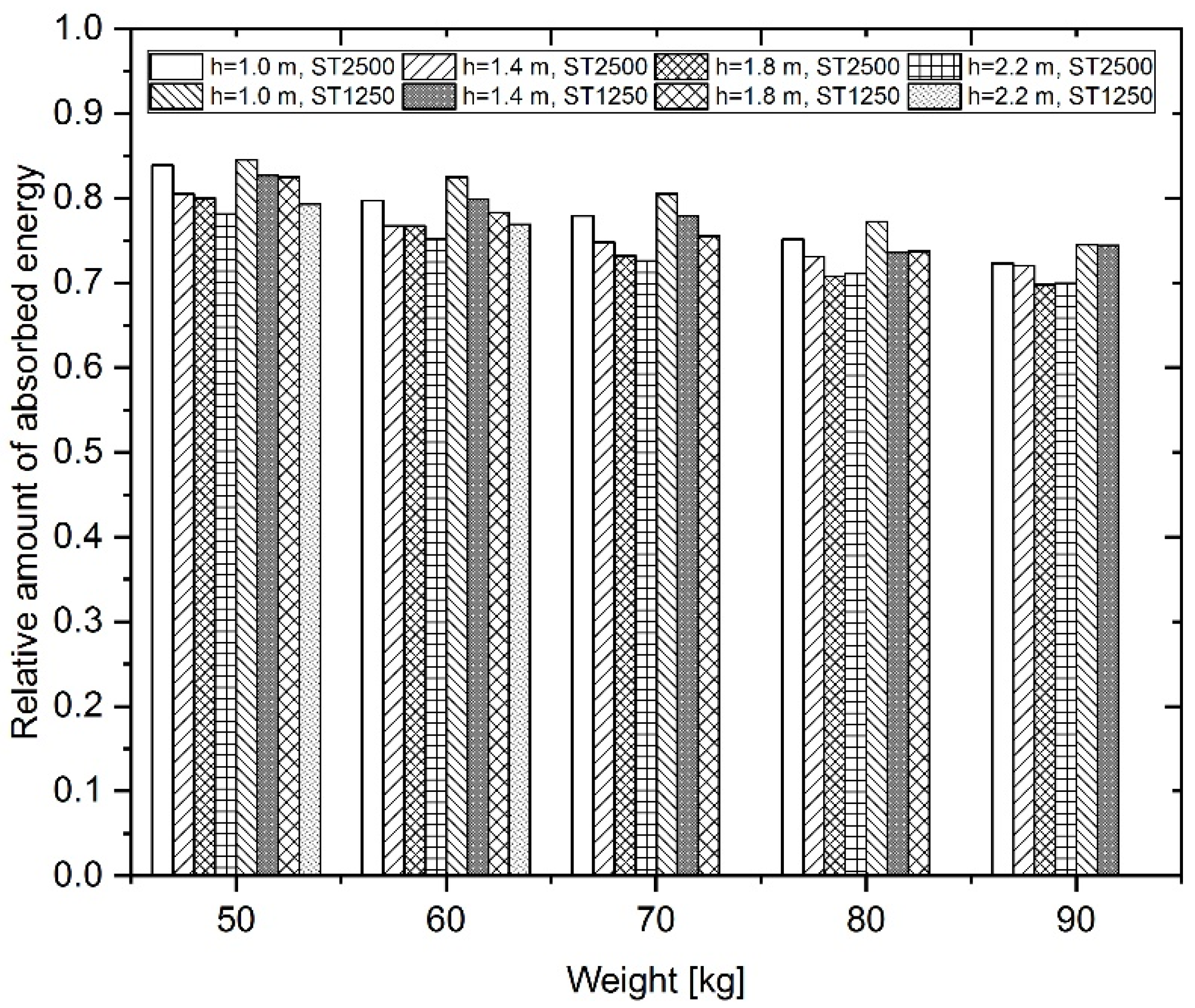
• The variable Conveyor belt type has the most significant influence on variable Y₃ (relative amount of absorbed energy) and also variable Y₄ (degree of damage).

4.3. Canonical Correlation Analysis

First, let us see if there is any correlation between the original variables. Since the variables were measured in different units, the relationships between them were identified using a correlation matrix (

Table 6. Correlation matrix of original variables.

	Weight	Height	Strength	Type *	Fimpact	ΔFtension	Erelat	Damage
Weight	1
Height	−0.050	1
Strength	0.057	0.0650	1
Type *	0.057	0.0650	−0.065	1
Fimpact	0.575	0.6042	0.274	0.332	1
ΔFtension	0.569	0.4985	−0.154	−0.347	0.585	1
Erelat	−0.296	−0.1046	−0.411	−0.787	−0.615	0.107	1
Damage	0.247	0.1418	−0.175	−0.397	0.065	0.456	0.246	1

* Reference category: Steel cord conveyor belt.

), where the relationship between the two variables was determined through the Pearson correlation coefficient r.

We used a scale to determine the degree of dependence: no correlation (|r| < 0.29), moderate correlation (0.30 <|r| < 0.49), medium correlation (0.50 <|r| < 0.79), and strong correlation (S, 0.80 <|r| < 1). If the correlation coefficient r is positive (or negative), there is a positive (or inverse) linear dependence between the variables. The results of the correlation matrix show that there is a strong inverse correlation between the variables E_relat and Type (r = −0.787) and also E_relat and F_impakt (r = −0.615). For the Type variable, the reference category was the steel cord conveyor belt. If the correlation coefficient is negative, the rubber textile conveyor belt acquires a value of the examined variable that is lower than that for the reference category, i.e., a steel cord conveyor belt (for example, in ΔF_n, E_relat, Damage). On the other hand, if the correlation coefficient is positive, the rubber textile conveyor belt acquires a value of the examined variable (for example, F_impakt) that is higher than that of the reference category. It turns out that there are moderate to medium correlations between many pairs of variables, which is enough for the data to be processed using the CCA method.

All the variables are divided into two groups. The first group of the original variables called Properties (Weight, Height, Strength, Type) describes the properties of the conveyor belt or the conditions of the experiment. The second group of variables called Result (impact force, increase in tension force, relative amount of absorbed energy, degree of damage) represent the variables describing the result of the conducted experiment. The first group represents the new canonical variable U and the second group the new canonical variable V. Verification of the statistical significance of canonical correlation analysis is carried out by means of several approximations of F-tests based on multivariate statistics (

Table 7. Significance test of canonical correlation analysis (α = 0.05).

Statistic	Value	Approx.F	Df	Error Df	p-Value
Wilks’ Lambda	0.0035	127.460	16	379.46	<0.0001
Pillai’s Trace	1.967	30.734	16	508	<0.0001
Hotellings	42.068	322.086	16	490.00	<0.0001

).

The tests confirmed that there is a statistically significant dependence (p-value < α) between the two groups of variables. That is, we reject the null hypothesis about the independence of the correlation coefficient.

In general, the number of canonical dimensions is equal to the number of variables in the smaller set. In our case, we have four pairs (roots) of canonical variables: $U_1$ and $V_1$, $U_2$ and $V_2$, $U_3$ and $V_3$, and $U_4$ and $V_4$. The number of significant pairs may be smaller. The next step is to verify the statistical significance of each pair of canonical variables by means of an approximative F-test and a Wilks’ lambda test (

Table 8. Test of canonical dimensions (α = 0.05).

	Rc	Rc2	F-Test	Df	Wilk’s Lambda	p-Value
1 to 4	0.9865	0.9731	127.460	16	0.0035	2.2 × 10−16
2 to 4	0.9206	0.8475	44.337	9	0.1302	2.2 × 10−16
3 to 4	0.3790	0.1436	5.186	4	0.8537	4.9 × 10−4
4 to 4	0.0558	0.0031	0.396	1	0.9969	0.5302 *

* p-value < alpha = 0.05.

). We test the null hypothesis that all pairs of canonical variables and uncorrelated, or $H_0:R_{c1}=R_{c2}=R_{c3}=R_{c4}=0$, where $R_{ci}$ is the canonical correlation coefficient for the ith pair of canonical variables, $i=\mathrm{1,2},3,4$. The estimated canonical correlations $R_c$ and the canonical coefficient of determination $R_c^2$ for all pairs are sorted by size.

The first value of the F-test in Wilk’s lambda statistical significance test (row 1 to 4, Table 8) tests the significance of all four canonical correlations. Since p-value < α, we reject the null hypothesis and assume that the first pair of canonical variables is significantly correlated. The second value of the F-test (row 2 to 4, Table 8) is used to test the significance of the second, third, and fourth canonical correlations, and the third value tests the significance of only the third and fourth canonical correlations. Finally, the last test is used to test whether the fourth canonical correlation is significant by itself (it is not, because p-value > α). It follows that only the first three pairs of canonical variables are statistically significant. The value of Wilks’ lambda is interpreted in the opposite direction to the canonical coefficient of determination $R_c^2$. A value close to zero indicates a high correlation, and vice versa, a value close to 1 indicates a low correlation.

The largest paired correlation coefficient is for the first pair of canonical variables $U_1$ and $V_1$ ($R_{c1}=0$.9865) and the second largest is for the pair $U_2$ and $V_2$ ($R_{c2}$ = 0.9206). The $R_c^2$ value can be interpreted similarly to the $r^2$ value in the regression analysis. We see that 97.31% of the variability of $V_1$ can be explained by the variability of $U_1$, and 84.75% of the variability of $V_2$ can be explained by the variability of $U_2$. Only 14.36% (or 0.07%) of the variability of $U_3$ (or $U_4$) can be explained by the variability of $V_3$ (or $V_4$). The first two pairs of canonical variables have a high canonical correlation and are the most important compared to the other pairs. Therefore, it is advisable to observe only the first two pairs of canonical variables. The canonical coefficients for canonical variable U and for canonical variable V for all canonical roots are in

Table 9. Raw canonical coefficients for variable U.

	U1	U2	U3	U4
Weight (X1)	−0.01739	0.014699	0.04854	−0.01417
Height (X2)	−0.87533	1.67473	−1.49463	0.77196
Strength (X3)	0.00077	0.00031	−0.00055	−0.00126
Type * (X4)	1.72555	0.47395	0.2268	0.88555

* Reference category: Steel cord conveyor belt.

and

Table 10. Raw canonical coefficients for variable V.

	V1	V2	V3	V4
Fimpact (Y1)	−0.000017	0.000178	−0.000409	−0.000095
ΔFtension (Y2)	−0.000064	−0.000013	0.000208	0.000117
Erelat (Y3)	−5.44905	−0.33918	−12.4333	−0.463445
Damage (Y4)	−0.22405	0.083297	0.115859	−2.11648

.

Since the original variables are not measured in the same units, it is recommended to use standardized canonical coefficients before raw canonical coefficients. These are standardized weightings that are chosen so that the condition of unit variances of canonical variables is satisfied. In practice, this means that the weightings are divided by the standard deviations of the corresponding canonical variables. In

Table 11. Standardized canonical coefficients for variable U.

	U1	U2	U3	U4
Weight (X1)	−0.2456	0.6635	0.6854	−0.2001
Height (X2)	−0.3481	0.6661	−0.5945	0.3070
Strength (X3)	0.4818	0.1971	−0.3448	−0.7896
Type * (X4)	0.8645	0.2374	0.1133	0.4436

* Reference category: Steel cord conveyor belt.

, there are standardized canonical coefficients for the canonical variable U and in

Table 12. Standardized canonical coefficients for variable V.

	V1	V2	V3	V4
Fimpact (Y1)	−0.0831	0.9029	−2.0751	−0.4810
ΔFtension (Y2)	−0.5124	0.1045	1.6507	0.9329
Erelat (Y3)	−0.7457	−0.0464	−1.7016	−0.0634
Damage (Y4)	−0.1230	0.0457	0.0636	−1.1619

, there are standardized canonical coefficients for variable V.

According to the absolute values of the standard canonical coefficients (Table 11 and Table 12), which we interpreted literally as weightings (increments) of canonical variables, we can conclude that the first canonical variable $U_1$ is most influenced by the variables Type and Strength. Variable $V_1$ is most strongly influenced by the variable E_relat (relative amount of absorbed energy) and variable ΔF_tension (increase in tension force). Variable $U_2$ is comparatively influenced by the variables Weight and Height, and variable $V_2$ is dominated by the variable F_impact (Impact force). It was discovered that in the first pair of canonical variables, the strength and type of conveyor belt are strongly inversely correlated with the increase in tension force and the relative amount of energy absorbed. In the second pair, the impact height and weight of the landing material are strongly positively correlated with the impact force.

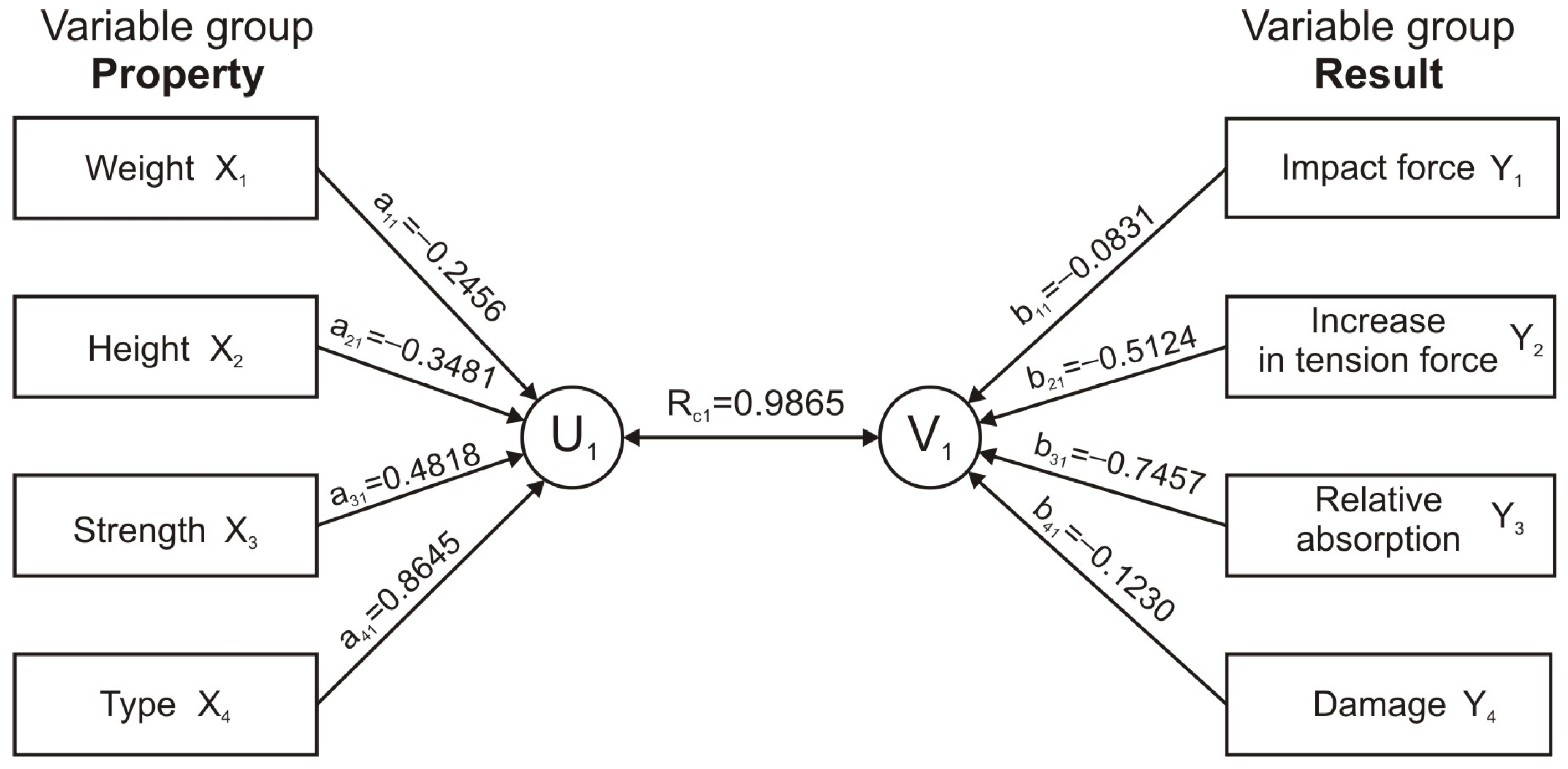
The first paired correlation coefficient has a value of 0.9865, which means that there is a strong relationship between properties (conditions) and the result of the experiment. Using the values of the standardized canonical coefficients in the first column of Table 11, the first canonical variable $U_1$ (or variable $V_1$ from Table 12) is determined using the following formula:

$$U_1=-0.2456X_1-0.3481X_2+0.4818X_3+0.8645X_4$$

(8)

$$V_1=-0.0831Y_1-0.5124Y_2-0.7457Y_3-0.1230Y_4$$

(9)

The graphical depiction of the canonical correlation analysis for the first canonical pair is shown in Figure 13. On the left side, there are the original variables, which form the canonical variable U, and on the right side, there are the variables forming the canonical variable V. The pair $\left(U_1,V_1\right)$ represents the first pair of canonical variables, the correlation of which is determined by the canonical correlation coefficient $R_{c1}$.

In an analogous way, we can determine other pairs of canonical variables, U and V. Standardized canonical coefficients are shown in Table 11 and Table 12.

The values of the canonical variables U and V are calculated using canonical coefficients. A graphical representation of the course of dependence between individual pairs of canonical variables is shown in Figure 14. The graphs confirm previous findings that the first two pairs of canonical variables have a high canonical correlation and are the most important compared to the other pairs.

A similar interpretation of variables is obtained by establishing a correlation between each variable and the corresponding canonical variable. In

Table 13. Correlation between original variables and canonical variables.

Variables	U1	U2	U3	U4	V1	V2	V3	V4
Weight	−0.151	0.655	0.702	−0.235	−0.149	0.603	0.266	−0.013
Height	−0.248	0.661	−0.643	0.294	−0.245	0.609	−0.244	0.016
Strength	0.389	0.263	−0.352	−0.809	0.384	0.242	−0.133	−0.045
Type *	0.797	0.306	0.136	0.503	0.786	0.282	0.052	0.028
Fimpact	0.067	0.917	−0.022	0.002	0.068	0.996	−0.028	0.029
ΔFtension	−0.688	0.597	0.107	0.006	−0.697	0.649	0.284	0.115
Erelat	−0.769	−0.534	−0.088	0.003	−0.780	−0.580	−0.232	0.047
Damage	−0.538	0.129	0.100	−0.044	−0.545	0.140	0.264	−0.783

* Reference category: Steel cord conveyor belt.

, there are the correlations (Pearson coefficient of correlation r) between the original variables determining the properties (or result) of the experiment and the canonical variables U and V.

For example, it follows (Table 13) that the first canonical variable $U_1$ is dominated by the variable Type (r = 0.797). The canonical variable $U_2$ is dominated by the variables Weight (r = 0.655) and Height (r = 0.661). The first canonical variable $V_1$ is dominated by the variables E_relat (r = −0.769) and ΔF_tension (r = −0.780). The canonical variable $V_2$ is dominated by the variable F_impact (r = 0.996). Table 13 is also supplemented by the correlation between the original input variables from the first group Property (or the second group Result) and the canonical variable V (or the variable U).

The explanation of canonical variables is complemented by the analysis of the variability and redundancy, the meaning of which lies in the expression of the proportion of the variability of variables of one group explained by the linear combination of the other group of variables (

Table 14. Analysis of variability and redundancy for both groups of original variables.

Canonical Variable Number	U (Feature)		Canonical Variable Number	V (Result)
	Variability	Redundance		Variability	Redundance
1	0.2119	0.2090	1	0.3396	0.3305
2	0.2182	0.2007	2	0.3745	0.3176
3	0.0377	0.0143	3	0.0075	0.0074
4	0.0008	0.0001	4	0.0005	0.0005
Total	0.4686	0.4241	Total	0.7221	0.6560

).

The total variability of the canonical variable U is 0.4686. This means that the canonical variable U is explained with 46.86% variability. The first two canonical variables are most involved in the explanation, with $U_1$ explaining 21.19% of the variability and $U_2$ explaining 21.82% of the variability. The other two canonical variables $U_3$ and $U_4$ together explain only 3.85% of the variability.

The total variability of the canonical variable V is 0.7221. This means that the canonical variable V is explained at 72.21% of the variability. The first two canonical variables are most involved in the explanation, with $V_1$ explaining 33.96% of the variability and $V_2$ explaining 37.45% of the variability. The last two canonical variables $V_3$ and $V_4$ together explain only 0.80% of the variability.

The total redundancy for the first group of variables determining the properties of the experiment (Properties) is 0.4241. That is, the variables of the second group determining the result of the experiment (Result) explain 42.41% the variability of the variables in the first group, and thereby the information about the first group is 57.59% redundant. The first two canonical variables $V_1$ and $V_2$ are most involved in explaining this variability, explaining 20.90% and 20.07% of the variability of the variables in the first group, respectively.

The total redundancy for the second group of variables (Result) is slightly higher, namely 0.6560. That is, the variables of the first group (Properties) explain 65.60% of the variability of the variables in the second group, signalling that they contain 34.4% of the excess information about the second group. The first two canonical variables, $U_1$ and $U_2$, are the most involved in explaining this variability, explaining 33.05% and 31.76%, respectively, of the variability of the variables in the second group.

5. Conclusions

The evaluation of the experimental research was carried out on 123 different samples of conveyor belts. The analysis of regression models shows that independent variables (weight of material, impact height, conveyor belt type and strength) significantly influence the output variables (impact force, increase in tension force, relative amount of absorbed energy, degree of damage). For example, the analysis of standardized coefficients of regression models shows the following:

• The impact height has a dominant influence on the impact force, followed by the weight of the falling hammer in second place.
• The most significant influence on the increase in tension force is from the weight of the falling hammer, which is a slightly greater influence than the impact height.
• The type of conveyor belt has the most significant influence on the relative amount of absorbed energy and also on the degree of damage to the conveyor belt.

In canonical correlation analysis, two groups of variables were created, the linear combination of which gave rise to new canonical variables U and V. The first four variables (weight of landing material, impact height, type and strength of conveyor belt) described the conduct and properties of the experiment. Four other variables (impact force, increase in tension force, relative amount of absorbed energy, degree of damage) described the outcome of the experiment. Canonical correlations showed strong links between these two groups of variables, with the canonical correlation coefficient as high as 0.9865 for the first canonical pair (0.9206 for the second canonical pair). In the first pair of canonical variables, the strength and type of conveyor belt dominate the first canonical variable U, and the second canonical variable V is dominated by the increase in tension force and the relative amount of absorbed energy. There is a strong inverse correlation between them. In the second pair, the impact height and weight of the impacting material correlate strongly and positively with the impact force.

Regression analysis determines the relationship between one output variable and several input independent variables. Canonical correlation analysis (unlike regression analysis) is a statistics method commonly applied to establish the relationship between two multidimensional datasets or variables using the correlation technique. Canonical correlation analysis is a certain generalization of multiple regression and correlation analyses. In this method, we transform a system of mutually correlated variables into a system of new variables. Both methods provide a different view of the dependencies between the observed variables, but the interpretation of the results is comparable.

From a practical point of view, we can conclude that the use of classical regression and correlation analysis is more advantageous. But on the other hand, canonical correlation analysis tracks the influence of multiple input and output variables and thereby gives a more comprehensive view of the result of the experimental research.

References

1. Guo, X.Q.; Liu, X.H.; Zhou, H.; Stanislawski, R.; Królczyk, G.; Li, Z. Belt Tear Detection for Coal Mining Conveyors. Micromachines 2022, 13, 449. [Google Scholar] [CrossRef]
2. Homisin, J.; Grega, R.; Molnar, V. Removal of systematic failure of belt conveyor drive by reducing vibrations. Eng. Fail. Anal. 2019, 99, 192–202. [Google Scholar] [CrossRef]
3. Sakharwade, S.G.; Nagpal, S. Analysis of Transient Belt Stretch for Horizontal and Inclined Belt Conveyor System. Int. J. Math. Eng. Manag. Sci. 2019, 4, 1169–1179. [Google Scholar] [CrossRef]
4. Fedorko, G. Application possibilities of virtual reality in failure analysis of conveyor belts. Eng. Fail. Anal. 2021, 128, 105615. [Google Scholar] [CrossRef]
5. Hu, X.; Zong, M. Fault Prediction Method of Belt Conveyor Based on Grey Least Square Support Vector Machine. In Proceedings of the 13th International Conference on Measuring Technology and Mechatronics Automation (ICMTMA), Beihai, China, 16–17 January 2021; pp. 55–58. [Google Scholar] [CrossRef]
6. Li, J.; Miao, C.Y. The conveyor belt longitudinal tear on-line detection based on improved SSR algorithm. Optik 2016, 127, 8002–8010. [Google Scholar] [CrossRef]
7. Qiao, T.; Chen, L.; Pang, Y.; Yan, G.; Miao, C. Integrative binocular vision detection method based on infrared and visible light fusion for conveyor belts longitudinal tear. Eng. Fail. Anal. 2017, 77, 93–101. [Google Scholar] [CrossRef]
8. Pang, Y.; Lodewijks, G. Large-scale conveyor belt system maintenance decision-making by using fuzzy causal modeling. In Proceedings of the 8th IEEE International Conference on Intelligent Transportation Systems (ITSC), Vienna, Austria, 16 September 2005; pp. 402–406. [Google Scholar] [CrossRef]
9. Li, X.G.; Zhang, Y.Z.; Zhan, Y.; Yang, L. Health State Prediction and Performance Evaluation of Belt Conveyor Based on Dynamic Bayesian Network in Underground Mining. Shock Vib. 2021, 2021, 6699611. [Google Scholar] [CrossRef]
10. Elahi, M.; Afolaranmi, S.O.; Lastra, J.L.M. Energy-Based Prognostics for Gradual Loss of Conveyor Belt Tension in Discrete Manufacturing Systems. Energies 2022, 15, 4705. [Google Scholar] [CrossRef]
11. Bajda, M.; Błazej, R.; Jurdziak, L. A new tool in belts resistance to puncture research. Appl. Mech. Mater. 2014, 683, 119–124. [Google Scholar] [CrossRef]
12. Bajda, M. Laboratory tests of conveyor belt parameters affecting its lifetime. Min. Sci. 2016, 23, 173–182. [Google Scholar] [CrossRef]
13. Bajda, M. Comparison of puncture resistance test results for different conveyor belt designs. In Proceedings of the 17th International Multidisciplinary Scientific Geoconference, SGEM 2017, Albena, Bulgaria, 29 June–5 July 2017; Volume 17, pp. 495–502. [Google Scholar] [CrossRef]
14. Komander, H.; Bajda, M.; Komander, G.; Paszkowska, G. Effect of strength parameters and the structure of steel cord onveyor belts on belt puncture resistance. Appl. Mech. Mater. 2014, 683, 119–124. [Google Scholar] [CrossRef]
15. Jurdziak, L.; Blazej, R.; Rzeszowska, A. Transverse Profiles of Belt Core Damage in the Analysis of the Correct Loading and Operation of Conveyors. Minerals 2023, 13, 1520. [Google Scholar] [CrossRef]
16. Honus, S.; Bocko, P.; Bouda, T.; Ristović, I.; Vulić, M. The effect of the number of conveyor belt carrying idlers on the failure of an impact place: A failure analysis. In Proceedings of the 17th International Multidisciplinary Scientific Geoconference, SGEM 2017, Albena, Bulgaria, 29 June–5 July 2017; Volume 17, pp. 125–132. [Google Scholar] [CrossRef]
17. Grincova, A.; Andrejiova, M.; Marasova, D. Failure analysis of conveyor belt in terms of impact loading by means of the damping coefficient. Eng. Fail. Anal. 2016, 68, 210–221. [Google Scholar] [CrossRef]
18. Grincova, A.; Andrejiova, M.; Marasova, D. Measuring and comparative analysis of the interaction between the dynamic impact loading of the conveyor belt and the supporting system. Measurement 2015, 59, 184–191. [Google Scholar] [CrossRef]
19. Kirjanów-Blazej, A.; Jurdziak, L.; Burduk, R.; Blazej, R. Forecast of the remaining lifetime of steel cord conveyor belts based on regression methods in damage analysis identified by subsequent DiagBelt scans. Eng. Fail. Anal. 2019, 100, 119–126. [Google Scholar] [CrossRef]
20. Jurdziak, L.; Blazej, R.; Kirjanów-Błażej, A.; Rzeszowska, A. Trends in the Growth of Damage Extents in a Steel Conveyor Belt’s Core. Minerals 2024, 14, 174. [Google Scholar] [CrossRef]
21. Song, B.; Zheng, C.; Jin, Y.; Shi, H.; Tao, Y.; Tan, S. A Fault-Targeted Gated Recurrent Unit-Canonical Correlation Analysis Method for Incipient Fault Detection. IEEE Trans. Ind. Inform. 2024, 20, 8739–8748. [Google Scholar] [CrossRef]
22. Lin, J.; Liu, H.; Huang, S.; Nie, Z.; Ma, H. Structural damage detection with canonical correlation analysis using limited sensors. J. Sound Vib. 2022, 538, 117243. [Google Scholar] [CrossRef]
23. Chen, C.; Geng, P.; Gu, W.; Lu, Z.; Ren, B. Assessment of tunnel damage potential by ground motion using canonical correlation analysis. Earthq. Struct. 2022, 23, 259–269. [Google Scholar] [CrossRef]
24. Liu, T.T.; Yu, X.H.; Lu, D.G. An Approach to Develop Compound Intensity Measures for Prediction of Damage Potential of Earthquake Records Using Canonical Correlation Analysis. J. Earthq. Eng. 2020, 24, 1747–1770. [Google Scholar] [CrossRef]
25. Jiang, Z.; Yuan, Q.; Lin, R.; Yang, F. Canonical Correlation Analysis and Visualization for Big Data in Smart Grid. IEEE J. Emerg. Sel. Top. Circuits Syst. 2023, 13, 702–711. [Google Scholar] [CrossRef]
26. Li, X.; Liu, Y.; Gao, Z.; Liu, D. Linkage between passenger demand and surrounding land-use patterns at urban rail transit stations: A canonical correlation analysis method and case study in Chongqing. Int. J. Transp. Sci. Technol. 2016, 5, 10–16. [Google Scholar] [CrossRef]
27. Zhou, Y.; Ma, G.; Zhang, H. Analysis of Relations between Transportation and Economic Development Based on Canonical Correlation Analysis. In Proceedings of the 4th International Conference on Economic Management and Model Engineering, ICEMME 2022, Nanjing, China, 18–20 November 2022. [Google Scholar] [CrossRef]
28. Zhao, S.; Gao, H.; Li, X.; Li, H.; Wang, Y.; Hu, R.; Zhang, J.; Yao, W.; Li, G. An outlier detection based two-stage EEG artifact removal method using empirical wavelet transform and canonical correlation analysis. Biomed. Signal Process. Control 2024, 92, 106022. [Google Scholar] [CrossRef]
29. Song, P.; Li, X.; Yuan, X.; Pang, L.; Song, X.; Wang, Y. Identifying frequency-dependent imaging genetic associations via hypergraph-structured multi-task sparse canonical correlation analysis. Comput. Biol. Med. 2024, 171, 108051. [Google Scholar] [CrossRef] [PubMed]
30. Huang, Y.; Zeng, P.; Zhong, C. Classifying brest cancer subtypes on multi?omics data via sparse canonical correlation analysis and deep learning. BMC Bioinform. 2024, 25, 132. [Google Scholar] [CrossRef]
31. Androniceanu, A.; Georgescu, I.; Tvaronaviciene, M.; Androniceanu, A. Canonical Correlation Analysis and a New Composite Index on Digitalization and Labor Force in the Context of the Industrial Revolution 4.0. Sustainability 2020, 12, 6812. [Google Scholar] [CrossRef]
32. Que, S.; Luo, H.; Wang, L.; Zhou, W.; Yuan, S. Canonical Correlation Study on the Relationship between Shipping Development and Water Environment of the Yangtze River. Sustainability 2020, 12, 3279. [Google Scholar] [CrossRef]
33. Vosoogh, A.; Saeedi, M.; Lak, R. Heavy metals relationship with water and size-fractionated sediments in rivers using canonical correlation analysis (CCA) case study, rivers of south western Caspian Sea. Environ. Monit. Assess. 2016, 188, 603. [Google Scholar] [CrossRef]
34. Andrejiova, M.; Grincova, A.; Marasova, D. Analysis of tensile properties of worn fabric conveyor belts with renovated cover and with the different carcass type. Eksploat. Niezawodn. 2019, 21, 472–481. [Google Scholar] [CrossRef]
35. Fedorko, G.; Molnar, V.; Marasova, D.; Grincova, A.; Dovica, M.; Zivcak, J.; Toth, T.; Husakova, N. Failure analysis of belt conveyor damage caused by the falling material. Part I: Experimental measurements and regression models. Eng. Fail. Anal. 2014, 36, 30–38. [Google Scholar] [CrossRef]
36. Grincova, A.; Andrejiova, M.; Marasova, D.; Khouri, S. Measurement and determination of the absorbed impact energy for conveyor belts of various structures under impact loading. Measurement 2019, 131, 362–371. [Google Scholar] [CrossRef]
37. Andrejiova, M.; Grincova, A.; Marasova, D. Failure analysis of rubber composites under dynamic impact loading by logistic regression. Eng. Fail. Anal. 2018, 84, 311–319. [Google Scholar] [CrossRef]
38. Kruskal, W. Concepts of relative importance. Questro 1984, 8, 39–45. [Google Scholar]
39. Fan, X.; Konold, T.R. Canonical correlation analysis. In The Reviewer’s Guide to Quantitative Methods in the Social Sciences; Taylor & Francis e-Library: New York, NY, USA, 2010. [Google Scholar]
40. Abdi, H.; Guillemot, V.; Eslami, A.; Beaton, D. Canonical Correlation Analysis. In Encyclopedia of Social Network Analysis and Mining; Alhajj, R., Rokne, J., Eds.; Springer: New York, NY, USA, 2018. [Google Scholar] [CrossRef]
41. Garson, G.D. Statnotes: Topics in Multivariate Analysis, Canonical Correlation. Available online: http://www2.chass.ncsu.edu/garson/ (accessed on 16 February 2010).
42. Johnson, R.A.; Wichern, D.W. Applied Multivariate Statistical Analysis; Prentice Hall: Upper Saddle River, NJ, USA, 1986; pp. 460–485. [Google Scholar]
43. Stankovicova, I.; Vojtkova, M. Multivariate Statistical Methods with Applications; Iura Edition: Bratislava, Slovakia, 2007. (In Slovak) [Google Scholar]
44. Van den Wollenberg, A.L. Redundancy analysis an alternative for canonical correlation analysis. Psychometrika 1977, 42, 207–219. [Google Scholar] [CrossRef]
Figure 1. (a) Test device, (b) hammer impactor, (c) support system.
Applsci 15 02639 g001
Figure 2. Sample fixation using hydraulically controlled jaws.
Applsci 15 02639 g002
Figure 3. (a) Rubber textile conveyor belt, (b) steel cord conveyor belt.
Applsci 15 02639 g003
Figure 4. The relative amount of energy absorbed [36].
Applsci 15 02639 g004
Figure 5. Examples of conveyor belt damage.
Applsci 15 02639 g005
Figure 6. Graphical representation of canonical correlation analysis.
Applsci 15 02639 g006
Figure 7. The time course of the impact force (m = 70 kg; h = 1.8 m).
Applsci 15 02639 g007
Figure 8. The time course of the tensile force (m = 70 kg; h = 1.8 m).
Applsci 15 02639 g008
Figure 9. Increase in tension force.
Applsci 15 02639 g009
Figure 10. The course of the hammer impact height over time.
Applsci 15 02639 g010
Figure 11. Relative amount of absorbed energy (rubber textile CB).
Applsci 15 02639 g011
Figure 12. Relative amount of absorbed energy (steel cord CB).
Applsci 15 02639 g012
Figure 13. First pair of canonical variables.
Applsci 15 02639 g013
Figure 14. Dependence between pairs of canonical variables.
Applsci 15 02639 g014