Random Forest-Based Stability Prediction Modeling of Closed Wall for Goaf

Abstract

To effectively mitigate the hazards posed by the blast waves of rock mass caving on closed walls during the mining process, a stability prediction method based on a random forest (RF) algorithm is proposed, which is designed to automatically identify key parameters. A machine learning model is developed using the algorithm, and its performance is evaluated through accuracy, precision, recall, and F1-score metrics. The probabilistic model of the objective function is constructed using the grid search hyperparameter optimization method, allowing for the selection of the most favorable hyperparameters for evaluation. The initial prediction accuracy of the RF algorithm model is 94.6%, indicating a strong predictive capability. Further adjustments to the base classifier, maximum depth, minimum number of leaves, and minimum number of samples enhance the model’s performance, resulting in an improved prediction accuracy of 95.9%. Finally, the optimized model is applied to predict the stability of the closed walls in the actual project, and the results are consistent with the on-site situation. This demonstrates that the random forest-based stability prediction model effectively forecasts the stability of closed walls in the actual project.

1. Introduction

Closed walls are essential structures in various engineering fields, including mining, civil engineering, and geotechnical engineering. They are designed to prevent the spillage of hazardous materials, such as fragments, chips, and magma, resulting from rock blasting, thereby reducing the risk of injuries, fatalities, and equipment damage during mining operations [1,2,3,4]. However, in situations such as roof falls, blasting activities, or accidents, shock waves can be generated that may impact the stability of these walls. Therefore, the accurate prediction of the impact of shock waves on closed walls is deemed crucial.

In the field of mining goaf management, the temporary or permanent closure of the goaf through the installation of closed walls is a major type of management measure. Types of closed walls include metal mesh, brick or masonry walls, concrete walls, and reinforced concrete walls. The study of the impact of air shock waves on closed walls due to the collapse of a mining area is a highly relevant and important topic in the field of mining engineering and geotechnical research. Badshah et al. [5] undertook a comprehensive set of eight blasting experiments involving various masonry wall configurations, namely, unreinforced masonry walls, wire mesh cement-covered masonry walls, and restrained masonry walls. The outcomes of these experiments served as a foundational platform for discerning the dynamic responses exhibited by each distinct masonry system in response to explosive forces. When the roof collapses and generates air shock waves in the goaf, the effect and damage law of the shock wave on the mine seal structure are different from the free field explosion because the underground roadway forms a relatively closed structure [6]. From the macroscopic perspective, the study of shock wave damage to mine seals concerns the mutual coupling effect between the shock wave and the underground structures [7]. Qu et al. [8,9,10] found that the overpressure law generated by a gas explosion is related to the propagation distance, cross-sectional area, and initial pressure of the burst source; they analyzed the damage effect of a gas explosion on underground structures. Kallu et al. [11] investigated the stability of a brick mine containment wall under the conditions of simultaneous blast loading and top and bottom slab displacement, and the results show that the deformation has an important influence on the blast resistance of the containment and should be considered in more detail in the design. Cheng et al. [12] studied the impact response of blast waves acting on mine structures after complex reflections or bypasses in the roadways by establishing numerical models of different types of bifurcated roadways and cornered roadways in mines.

Given the high cost of acquiring explosion data and the challenges associated with experimental validation, numerical simulation is becoming an increasingly preferred method [13,14,15,16,17,18]. Numerical simulation offers a valuable and cost-effective way to analyze the complex dynamics of masonry structure failure under the impact of blast waves. Numerous scholars have conducted research on the fragment distribution, size, ejection patterns, and damage assessment of unidirectional masonry walls subjected to shock waves through experiments and numerical simulations [7]. Traditional methods for assessing the stability of closed walls are typically based on hand calculations or simple models, which may overlook the influence of complex geological and engineering conditions on the stability of these walls, resulting in predictions that are less accurate or reliable. Zhang et al. [13,19] used numerical simulation to study the propagation law and pressure distribution of shock waves in the bends of a roadway and found that the decay of peak overpressure with distance did not obey the exponential law when air shock waves passed through the bends of the roadway. Utilizing the discrete element method (DEM), Masi et al. [20] investigated the dynamic response of curved masonry structures under blast loading and the effects of the shear expansion angle and tensile strength on the dynamic structural response of masonry. Edri and Yankelevsky [21] developed a resistance model and single-degree-of-freedom (SDOF) computational method for unidirectional hollow concrete block-filled brick walls by simulating an unreinforced masonry wall, which can predict the response of this masonry wall under different types of out-of-face static loads. Dong et al. [22] investigated the damage of the roof impact wave on an ore column using theoretical modeling. Geng et al. [23] proposed a simulation model of roof fall in an underground mined-out area based on lattice Boltzmann, which provides a new approach for predicting the disaster of roof fall in mined-out areas. Wang et al. [24,25,26] used mathematical methods to carry out a study of stability prediction for the stability of the roof plate of a mined-out area. Zhao et al. [27] used the numerical software (ANSYS Fluent 2023 R1) of fluid dynamics to simulate and analyze a roof slab fall in a mining goaf area. Xing et al. [28,29] established a coupled roof fall/air impact model to study the influence of the roof height on the air velocity of the quarry and the roadway when the roof falls. Rodriguez et al. [30,31,32] investigated the effects of downhole shock waves on different shapes of wave-retarding walls through experiments and numerical simulations. Rajasekar et al. [33] investigated the effect of different-shaped geometric barriers on mitigating shock waves and their numerical prediction methods using similar simulation experiments and numerical simulations.

Furthermore, recent research has been leaning towards using techniques that combine AI-driven approaches and multi-physics coupling for prediction, yielding many promising results. Sha et al. [34] utilized a multi-physics coupling prediction model to develop a fluid–solid coupling model based on asymmetric rock strata structures, considering dynamic geological responses (Rock Mechanics and Rock Engineering), achieving a 38% reduction in the prediction error compared to traditional models. Xi, Dongmin, et al. [35] proposed a cross-mining area transfer learning framework in “Tunnelling and Underground Space Technology” using an AI-driven approach to address small sample problems (achieving a 90% accuracy with only 150 data points); BYD’s mining AI platform employs multi-modal data fusion to integrate microseismic, InSAR, and laser scanning data to predict collapse risks in real time (measured response time < 12 s). Jiang et al. [36] proposed Physics-Informed Neural Networks (PINNs) using a physics mechanism and data-combined modeling approach. By constructing a PINN model with constitutive constraints for rock mass damage, they achieved a 24% reduction in error compared to purely data-driven methods. These latest approaches have greatly advanced the research in related fields.

Against this backdrop, machine learning methods offer a novel approach to overcome the limitations of numerical simulations. The random forest (RF) algorithm, through its ensemble learning strategy, can efficiently process multi-source heterogeneous data and capture nonlinear relationships between variables. By inputting finite element simulation data as a training set into the RF model, rapid surrogate predictions of the structural response can be achieved. Furthermore, RF models exhibit greater robustness in parameter sensitivity analysis, making them particularly suitable for mining scenarios with complex geological conditions and sparse monitoring data. This paper selects the random forest model precisely because of its complementarity with the finite element method—the latter provides physics-driven, refined simulation data, while the former achieves efficient prediction through a data-driven approach. The combination of these two can provide a multi-scale solution for the stability assessment of retaining walls.

The scholars mentioned above have conducted extensive research on roofing disasters and the stability of the mining zone, yielding significant results. However, there are still many challenges in practical application. Most existing prediction models are complex to build, require a large amount of data to be collected, and are difficult to deploy in practice, and many theoretical analyses and numerical simulations rely on simplified assumptions, often overlooking the complexities of the actual environment, such as material non-homogeneity and variations in the ambient temperature and humidity. Additionally, experimental conditions have some limitations. The experimental research is often limited by experimental conditions and equipment, making it difficult to fully simulate actual working conditions. In particular, large-scale explosion simulation experiments are costly and risky, which further constrains their applicability. Moreover, there is a lack of long-term performance evaluation, as most research focuses on the effects of transient impact and short-term loading, and there is a lack of systematic research on the environmental erosion and fatigue damage suffered by closed walls in the course of long-term use.

The shock wave generated by a roof fall in a mined-out area seriously affects the quarry stability and personnel safety. To investigate the effects of these shock waves on sealing protection requirements, data on the shock wave sizes generated by roof falls in various mined-out areas and the mechanical parameters of the closed walls were systematically collected. An RF algorithm was employed to fit the influence of the mechanical parameters of the closed walls and the shock wave size on the construction area under their coupled effects. The safety threshold values for the mechanical parameters of the closed walls were accurately predicted under the pressure of shock waves generated by roof falls in different mined-out areas, thereby providing technical guidance for similar engineering practices.

In this study, we propose the following four research hypotheses: (1) the mechanical parameters and shock wave velocity jointly influence the stability of confined walls; (2) the random forest model can effectively capture nonlinear relationships; (3) hyperparameter optimization can significantly improve the model accuracy; (4) the model possesses practical engineering applicability. Based on these hypotheses, a closed wall damage prediction model based on an RF algorithm is proposed, and the hyperparameters are optimized using a grid search to enhance the model prediction performance. A random forest algorithm model is trained for prediction, and the trained machine learning model is further tuned with hyperparameters. The contributions of this research are as follows: (1) the development of an efficient damage prediction model for confined walls; (2) the introduction of a model hyperparameter optimization algorithm combining a grid search method; (3) the proposition of an efficient prediction model based on the random forest algorithm for predicting the extent of damage to confined walls in engineering instances; (4) experimental validation of the proposed model based on actual working conditions.

2. Experimental Data Description

2.1. Experimental Data Contents

The experimental data used in this study were collected from three operating underground metal mines (copper and silver polymetallic mines), none of which were abandoned. The mines included stope heights ranging from 5 to 30 m and employed combined rock bolt and shotcrete support. The confined walls were constructed from C20–C30 concrete. On-site data acquisition, using pressure sensors and laser velocimeters, focused on the following four main areas: the shock wave velocity, compressive strength of the confined walls, shear strength of the confined walls, and hazard level. These four components will be described in detail in the following sections. The dataset is publicly available; contact the authors for access.

2.1.1. Shock Wave Velocity

The extent of damage to mine walls caused by shock waves primarily depends on their velocity; therefore, this paper collected data on shock wave velocities. During mining activities, the roof of a mined-out area can collapse due to rock damage or destabilization. The process of roof collapse is similar to the piston movement, which aligns with the pump model. In this model, the rock wall (side gang) acts as the pump, while the falling rock mass serves as the piston, as shown in Figure 1. When the roof collapses, the falling rock body releases a significant amount of energy while compressing the air inside the mined-out area, and continues along the roadway in the form of waves dramatically discharged to form a shock wave. Then, the closed wall is damaged by the pressure and amplitude of the shock wave, causing it to deform, crack, or collapse, thus affecting the stability of the closed wall.

The magnitude of the shock wave generated during a roof fall in a mined-out area is typically expressed as the maximum velocity v_max. This velocity is influenced by factors such as the height of the mining area, the exposed area, and the total area of the roadway leading to the mined-out area. According to the “pump” model, the movement of the falling rock can be regarded as a free falling, and the mined-out area and the falling rock can be regarded as a cylinder and a piston, respectively. In this context, v_max can be calculated using the following equation:

$${\nu }_{\max }={\displaystyle \frac{\eta S_k\sqrt{2gH}}{S_a+(1-\eta )S_e}}$$

(1)

where η is the whole-layer disintegration coefficient of the roof plate in the mined-out area, and its value is related to the rock layer of the roof plate and the exposed area. Specifically, the stronger the surrounding rock, the larger the exposed area and the higher the value. S_k is an exposed area of the mined-out area, g is the gravity acceleration, H is the height of the roof plate, S_a is the sum of all of the broken areas of the roadway connected with the mined-out area, and S_e is an exposed area of the roof plate.

From Equation (1), it is evident that the maximum velocity of the shock wave is positively correlated with the exposed area and the height of the roof plate in the mined-out area, while it is negatively correlated with the total cross-sectional area of all roadways connected to the mined-out area. Based on the conversion relationships between the wind speed and force (Equations (2) and (3)), and referencing the blasting safety regulation “GB 6722-2014” [37], the degree of injury to the human body from impact airflow is shown in

Table 1. Human injury from shock wave overpressure.

Shock Wave Overpressure/MPa	Degree of Damage	Injuries
0.02~0.03	minor	contusion
0.03~0.05	medium	organ damage
0.05~0.1	serious	possible death
>0.1	extremely serious	deaths

(under the standard conditions, the air gravity r = 0.01225 kn/m³, and the gravitational acceleration g = 9.8 m/s²).

$$F=\rho Q(V_2-V_1)$$

(2)

$$Wp={\displaystyle \frac{0.5r{v}^2}{g}}$$

(3)

In Equation (2), F represents the force, ρ represents the fluid density, Q represents the volumetric flow rate, V₂ represents the outlet velocity, and V₁ represents the inlet velocity. This formula can be used to calculate the force generated by the fluid due to the change in its velocity. Meanwhile, in Equation (3), Wp represents the pressure head, r represents the radius, v represents the fluid velocity, and g represents the acceleration due to gravity. This formula converts the fluid’s velocity into a pressure head, and is used to estimate the pressure and energy loss.

2.1.2. Input Factors

The closed wall plays an important protective role in the process of roof fall, as it mitigates the impact of a shock wave and guarantees the safety of both the engineering structures and personnel. The compressive strength and shear strength of the closed wall are chosen as the important indices for evaluating the damage to the surrounding rock and its equipment caused by the shock wave generated from the roof slab fall.

Assuming there is no water accumulation situation in the mined-out area, the calculation of the closed wall thickness focuses on the roof plate of the mined-out area, which generates the shock wave pressure. According to the calculation formula of two different design strengths, the thickness of the closed wall in different mined-out areas can be calculated, taking C₂₀ concrete as an example. The specific formula is shown below:

(1)

Calculated by compressive strength.

$$B=\left\{{\left[{(a+b)}^2+4pab/f_c\right]}^{1/2}-(a+b)\right\}/(4\tan \alpha )$$

(4)

where B is the thickness of the closed wall, in m; a is the width of the roadways where the closed wall is located, taking the value of 2.4 m; b is the height of the roadways where the closed wall is located, taking the value of 2.6 m; p is the hydrostatic pressure on the closed wall, with the air shock wave pressure being 10 times, in MPa; f_c is the value of the compressive strength of concrete, taking the value of 9.5 MPa; and α represents the angle of shock wave propagation, and its specific value depends on the specific conditions of the goaf.

(2)

Calculated by shear strength.

$$B\ge pab/2\left(a+b\right)f_v$$

(5)

where f_v is the shear strength of C₂₀ concrete, taking the value of 2.369 MPa.

The data presented above are derived from the actual conditions of the mining area where the dataset was collected, as well as the “Code for Design of Concrete Structures” (GB 50010-2010) [38]. Specifically, the dimensions of the roadway (a = 2.4 m; b = 2.6 m) are determined based on the statistical average of actual engineering design cases in mines. The compressive strength (f_c = 9.5 Mpa,) and shear strength (f_v = 2.369 Mpa) of C20 concrete are cited from the “Code for Design of Concrete Structures” (GB 50010-2010).

Based on the organization and analysis of the existing database, combined with the current prediction model, the following three characteristic parameters were finally identified as inputs for predicting the shock wave speed (m/s, where the symbol is SPEED), the compressive strength (MPa, where the symbol is σbc), and the shear strength (MPa, where the symbol is τ). The damage level of the closed wall was classified as no damage, slight damage, or severe damage.

Figure 2 presents the pairwise relationships of the input parameters, illustrating the relationships between the three variables (SPEED, σbc, and τ) in a pairwise manner, and color-coded according to the “Damage” level. The plots on the diagonal show the distribution of each variable, using kernel density estimation (KDE) plots. Different colors represent different damage levels, allowing for the observation of the distribution of each variable under different damage levels. For example, “SPEED” exhibits a more dispersed distribution at damage level 1, while it is more concentrated and has larger values at damage level 3. The off-diagonal plots display the scatter plot relationships between two variables. The color coding also indicates the damage level. For instance, in the scatter plot of “SPEED” and “σbc,” a positive correlation can be observed, and as the damage level increases, the values of both variables also increase accordingly. The pairwise relationship plot in Figure 2 reveals a significantly strong correlation among the three input parameters: SPEED, σbc, and τ. This indicates that the input parameters are strongly correlated, enabling the model to better capture their inherent connections. This interconnected information provides richer features for the model, assisting it in more accurately understanding the data patterns, thereby enhancing the accuracy and reliability of the predictions. Therefore, using these three features from the dataset in this paper is reasonable.

2.1.3. Confined Wall Damage Levels

In all of the datasets used in this paper, the confined wall damage levels are classified into the following three categories: no damage, minor damage, and serious damage. We used these three damage levels to assess the safety of confined walls, and these levels served as labels for evaluating the performance of the research methods presented in this paper.

2.2. Dataset Splitting

The data used in this study are based on the systematic collection of 167 groups of dimensions from different mined-out areas within the mine, along with the mechanical data of the closed wall. Among these, 94 groups acted on the closed wall with no damage, 52 groups with slight damage, and 21 groups with severe damage. The distribution pie chart is shown in Figure 3. Each group includes the shock wave speed, and the compressive strength and shear strength of the closed wall, along with the corresponding damage level. Following established practices in data segmentation, 80% of the data were randomly selected for the training set to develop the machine learning model (which consists of 75 sets of undamaged data, 42 sets with slight damage, and 17 sets with severe damage), while the remaining 20% were reserved for the test set to evaluate the accuracy of the trained model (comprising 19 undamaged, 10 slightly damaged, and 4 severely damaged cases). The training set (134 cases) was used for the model construction and hyperparameter optimization. Actual hyperparameter optimization was performed via ten-fold cross-validation within the training set, without using any data from the test set. The test set (33 cases) was solely used for the final performance evaluation.

Figure 3 uses horizontal stacked bar charts and a pie chart to represent the distribution and proportion of data for each category within the dataset, training set, and test set. In the overall dataset, samples with no damage are predominant, followed by slight damage, with the fewest samples exhibiting severe damage. The proportions in the training and test sets are generally consistent with those in the dataset, ensuring that the model does not bias toward a particular category during training, thereby improving its generalization ability across different damage levels.

2.3. Variable Influence

The Pearson correlation coefficient is used to measure the linear relationship between fixed-distance variables, and its value is between −1 and 1. Figure 3 displays the Pearson correlation coefficients for each parameter. The positive correlations between the damage degree of the closed wall and the shock wave speed, compressive strength (MPa), and shear strength (MPa) indicate that the damage degree is positively correlated with these three input variables, with the strongest correlation observed between the shock wave speed and damage degree. Figure 4 displays the heatmap of the correlation coefficients between each variable. As can be seen from the figure, the correlation between each variable is relatively high. Specifically, a very strong positive correlation exists between the shock wave speed (SPEED), compressive strength (σbc), and shear strength (τ) (correlation coefficients close to 1), indicating a high degree of linearity among these variables, where an increase in one often accompanies increases in the others. A positive correlation also exists between the shock wave speed (SPEED), compressive strength (σbc), and shear strength (τ) and the damage level (Damage) (correlation coefficients ranging from 0.80 to 0.87), suggesting that increases in these variables can lead to an increase in the degree of damage. Therefore, it can be stated that the damage to the closed wall is not determined by a single variable, but rather by the combined effects of multiple variables. This demonstrates that the parameters we used are useful for making meaningful and reasonable predictions.

3. Stability Prediction Model

3.1. Predictive Modeling

The modeling steps for the random forest approach are summarized as follows:

(1)

Data acquisition and preprocessing: obtain a dataset containing features and target variables and perform preliminary data processing.

(2)

Data splitting: divide the preliminarily processed dataset into a training set and a test set using an appropriate sampling method, according to a certain ratio (this study uses an 8:2 ratio for data partitioning). Randomly select samples from the training set to construct multiple decision trees. The results of all of the decision trees can then be integrated through voting or averaging to generate prediction results.

(3)

Model evaluation and optimization: use the test set to evaluate the model performance by considering the accuracy, precision, recall, and other indicators; based on the evaluation results, adjust the model parameters to achieve the final model optimization.

Using Python version 3.8.20, the model was developed with the RF classification algorithm, leveraging geological parameters (the dimensions of the roadway, which was used in Section 2.1.1 for calculating the shock wave velocity) of a mined-out area and mechanical parameters (the compressive strength σbc and the shear strength τ) of the closed wall as features to predict the impact of the shock wave from roof fall under various conditions. The model employs several scikit-learn modules, such as the ensemble module for the random forest classifier, the neural_network module for the multilayer perceptron (MLP) classifier, and the model_selection module for splitting the dataset into training and test sets, performing cross-validation, and tuning. The metrics module is used to compute the model accuracy and confusion matrices for evaluation. Further hyperparameter optimization enhanced the performance of the prediction model, demonstrating that the RF algorithm, especially after optimization, exhibits an excellent predictive capability. In this study, there is no mathematical derivation for the machine learning model, so only the RF algorithm is introduced.

3.2. RF Algorithm

The RF algorithm is a widely used ensemble learning method that combines multiple decision tree algorithms. As a form of parallel integration, it effectively prevents overfitting and is well suited to classifying high-dimensional data. It is robust, accommodates unbalanced datasets, and achieves a high classification accuracy.

The steps of the RF algorithm are generally as follows: First, the best features are selected for splitting based on metrics such as Gini impurity or information gain, allowing for the construction of multiple decision trees. In the training process, each decision tree is built by randomly selecting some features for training. When classifying the training samples, the RF algorithm aggregates the classification results from all decision trees and selects the category with the most votes as the final classification result. With its high flexibility, strong performance, and ability to handle complex nonlinear relationships, the random forest algorithm has become one of the important tools in machine learning, and has been widely used in the geosciences in recent years, obtaining excellent results.

4. Hyperparameter Optimization

4.1. Overview of Hyperparameters and Optimization Methods

Parameters that must be set before training a model are known as hyperparameters. Certain hyperparameters in machine learning predictive models influence the training process and directly impact the expected performance of the model. Key hyperparameters include the learning rate, number of dense layers, number of dense nodes, activation functions, learning level, and maximum depth in machine algorithm models, all of which are evaluated through grid search optimization. Different machine learning methods have different hyperparameter settings. In this study, the default base learner used in the RF algorithm is the decision tree model, with the following default hyperparameters and initial values: base classifiers (n_estimators) at 200, a maximum depth (max_depth) of 2, a minimum number of samples (min_samples_split) of 20, and a minimum number of leaves (min_samples_leaf) of 8.

The model was fine-tuned during training using ten-fold cross-validation and a grid search for the hyperparameter optimization.

During the grid search process, the performance of each hyperparameter combination was evaluated using 10-fold cross-validation. The specific steps are as follows:

(1)

Randomly divide the training set (117 data points) into 10 subsets.

(2)

Sequentially select one subset as the validation set, and the remaining nine subsets as the training subsets.

(3)

For each hyperparameter combination, calculate the average accuracy across the 10 validations as the performance metric.

(4)

Select the hyperparameter combination with the highest average accuracy as the optimal configuration.

Hyperparameter optimization was performed using 10-fold cross-validation on the training data rather than using an independent validation set. The test set was used only for the final model performance evaluation. Ten-fold cross-validation ensures that all of the data points are used for both the training and test sets, allowing for a comprehensive evaluation. The grid search searches all of the combinations of candidate hyperparameter values, compares their effectiveness, and identifies the optimal combinations to enhance the model prediction performance. The results obtained through ten-fold cross-validation and grid search training are thus more reliable and robust.

4.2. Hyperparameter Combination Selection

A total of four hyperparameters were selected for optimizing the RF algorithm. These include four possible values for n_estimators, four possible values for the maximum depth, four possible values for min_samples_leaf, and three possible values of min_samples_split, resulting in a total of 192 unique combinations. The candidate values for these hyperparameters are close to the default settings, as shown in

Table 2. Hyperparameters of the grid search RF algorithm.

Algorithms	n_Estimators	max_Depth	min_Samples_Leaf	min_Samples_Split
RF	200	2	4	10
	250	4	6	20
	300	6	8	30
	500	10	10	40

.

5. Results and Discussion

5.1. Evaluation Metrics Description

In machine learning, model evaluation is essential and occurs at two levels. First, during the model training process, the training set is used to evaluate the model with different parameters, aiming at optimizing these parameters. Second, once the model is built, it is evaluated using the test set to verify the final performance. This two-tiered approach ensures both effective training and the reliable assessment of the model’s predictive capabilities.

To gain a comprehensive understanding of the performance of the classification model, test sets are often utilized to analyze the detailed predictions through confusion matrices. These matrices display the number of true positives, false positives, true negatives, and false negatives, which helps to deeply analyze the model’s performance in each category and make more targeted adjustments. In binary classification problems, the two categories are classified as positive or negative. In multi-class scenarios, the definitions of positive and negative are relative: any category can be treated as positive, while the remaining categories are considered negative.

All of the results appearing in the model can be categorized into the following four types: (1) true positive (TP) occurs when the true value is positive and the predicted value is also positive; (2) false negative (FN) arises when the true value is positive but the predicted value is negative, representing a Type I error; (3) false positive (FP) occurs when the true value is negative while the predicted value is positive, which is known as a Type II error; and (4) true negative (TN) is when both the true and predicted values are negative.

These four cases can be organized into a table, resulting in what is known as a confusion matrix. While the confusion matrix effectively counts the number of positives and negatives, it can be challenging to evaluate the strengths and weaknesses of the model solely based on case counts, especially with large datasets. Therefore, additional key performance indicators are introduced to provide a more comprehensive assessment.

Precision indicates the proportion of positive predictions made by the model that are actually correct. It measures the probability that a predicted positive outcome is accurate, calculated as the number of true positives (TPs) divided by the sum of true positives and false positives (TPs + FPs).

Recall, also known as sensitivity, measures the proportion of actual positive cases that the model correctly identifies. It is calculated as the number of true positives (TPs) divided by the sum of true positives and false negatives (TPs + FNs). A higher recall indicates that the model is effective at capturing more positive samples, thus reflecting its ability to minimize missed positive cases.

F1-score is the harmonic mean of precision and recall, providing a single metric that balances both aspects of the model performance. It ranges from zero to one, where a higher F1-score indicates a better overall classification quality.

The accuracy, precision, recall, and F1-score are indicated below as follows:

Accuracy = (TP + TN)/(TP + FP + TN + FN)

(6)

Precision = TP/(TP + FP)

(7)

Recall = TP/(TP + FN)

(8)

F1 = 2 × Precision × Recall/(Precision + Recall)

(9)

5.2. Hyperparameter Optimization Results

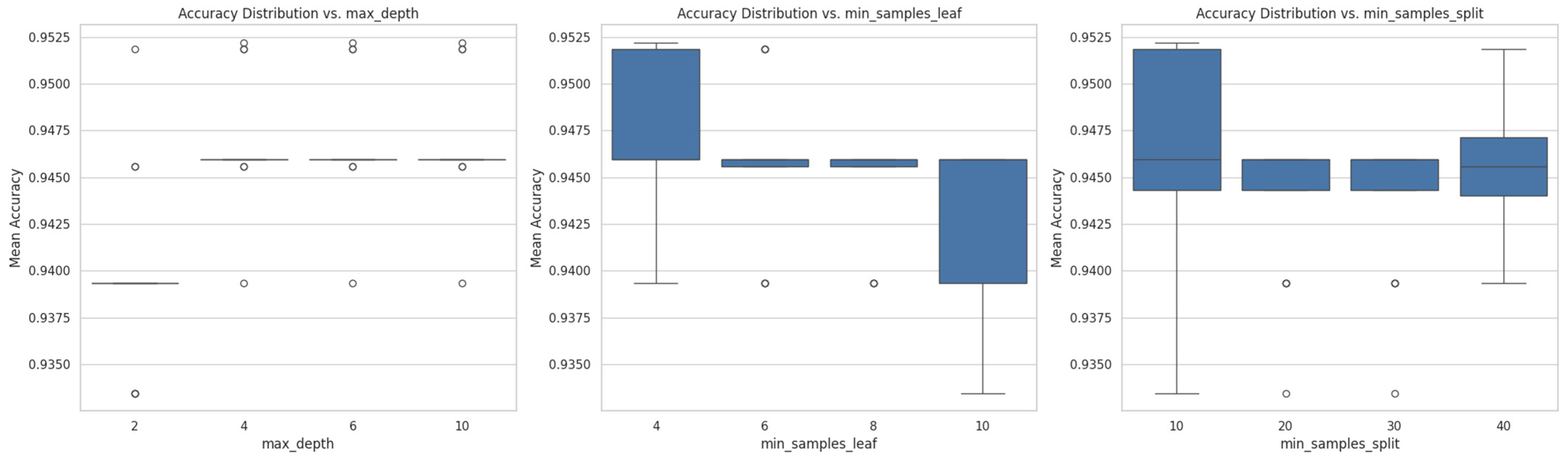
Figure 5 shows the impact curves of various parameters on the model’s accuracy. The curves in the figure were obtained by fixing the x-axis parameter and then calculating the average prediction accuracy of all other parameter combinations. From the figure, it can be seen that the prediction accuracy of n_estimators = 250 is significantly higher than other values. The relatively optimal parameter combination is as follows: n_estimators = 250, max_depth = 4, min_samples_leaf = 4, and min_samples_split = 10, which is consistent with the hyperparameter optimization results.

Since averaging cannot determine the optimality of the selected parameters, we further analyzed the parameters. Taking n_estimators = 250, we analyzed the prediction accuracy of different parameters for max_depth, min_samples_leaf, and min_samples_split. The resulting box plot is shown in Figure 6. It can be seen that the parameters obtained by hyperparameter optimization are indeed superior to the other parameter combinations. The best combination of parameters for the RF algorithm is shown in

Table 3. Best hyperparameter combination with the random forest algorithm.

Model	Hyperparameters	Number	Accuracy
RF	n_estimators	250	0.959
	max_depth	4
	min_samples_leaf	4
	min_samples_split	10

, with the accuracy being the average accuracy of ten-fold cross-validation. Compared to the parameter combination of n_estimators = 200, max_depth = 0, min_samples_leaf = 4, and min_samples_split = 10, the prediction accuracy of the learning curve and the test curve for this parameter increased from 94.6% to 95.9%.

After grid search hyperparameter optimization, the RF model exhibited significantly improved prediction performance. This method effectively selects the optimal parameters that enhance the accuracy of the model. As a result of this hyperparameter optimization, the RF algorithm achieves more precise predictions, demonstrating its efficacy in refining model performance.

5.3. Performance of Machine Learning Techniques Results

After the hyperparameter optimization, the optimal prediction accuracy and other metrics for the random forest-based closed wall damage prediction model are as shown in

Table 4. Prediction performance table of the random forest model on the training set.

	Accuracy	Recall	F1	Average
No damage	0.99	0.97	0.98	0.959
Minor damage	0.93	0.95	0.94
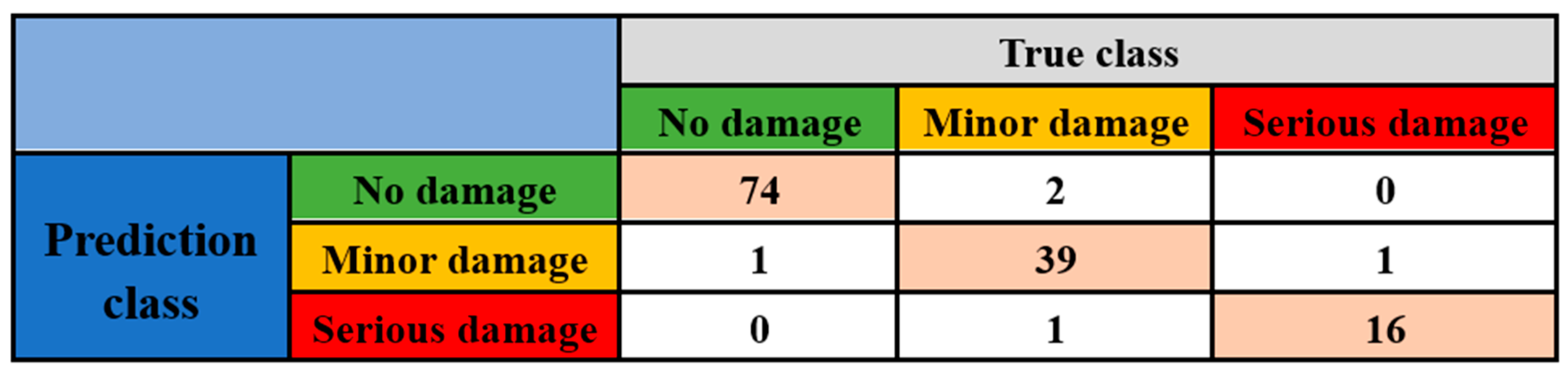
Serious damage	0.94	0.94	0.94

. The trained RF algorithm achieved an accuracy of 96%, with a prediction accuracy of 0.99 for the no damage class, a recall of 0.97, and an F1 value of 0.98. For the minor damage class, the prediction accuracy is 0.93, the recall is 0.95, and the F1-score is 0.94. In the severe damage category, the prediction accuracy is 0.94, the recall is 0.94, and the F1-score is also 0.94. The weighted averages for the accuracy, recall, and F1-score are 0.95, 0.96, and 0.95, respectively. The model identified six misjudgment groups in the test set, including one for no damage, two for minor damage, and three for serious damage. The confusion matrix for each model is presented in Figure 7.

The experimental results show that, by using grid search to optimize the hyperparameters, a high prediction accuracy can be achieved with the RF algorithm. Compared to traditional prediction methods, this approach offers comparable predictive performance but is simpler and easier to deploy.

To test the robustness of the algorithm, its performance was validated on the test set. The confusion matrix of the RF model on the test set is shown in Figure 8. The performance results are shown in

Table 5. Prediction performance table of the random forest model on the test set.

	Accuracy	Recall	F1	Average
No damage	0.95	0.95	0.95	0.95
Minor damage	0.90	0.90	0.90
Serious damage	1.00	1.00	1.00

.

The experimental results on the test set show that the model can still maintain a 95% accuracy on the test set. The performance degradation is not significant, indicating strong robustness.

In this study, a machine learning modeling algorithm for predicting the stability of closed walls was proposed by combining the recent development of the RF model and ML methods. The results obtained in this study will help to encourage the use of machine learning in the prediction of closed wall stability, which can be useful for engineering geology-related fields.

However, the method presented in this paper does not account for the influence of temperature and humidity on the stability of confined walls. Experimental results may vary under different environmental conditions. Future work could explore hybrid modeling incorporating physical models to consider more influencing factors, evaluate the algorithm’s feasibility, and address potential issues accordingly.

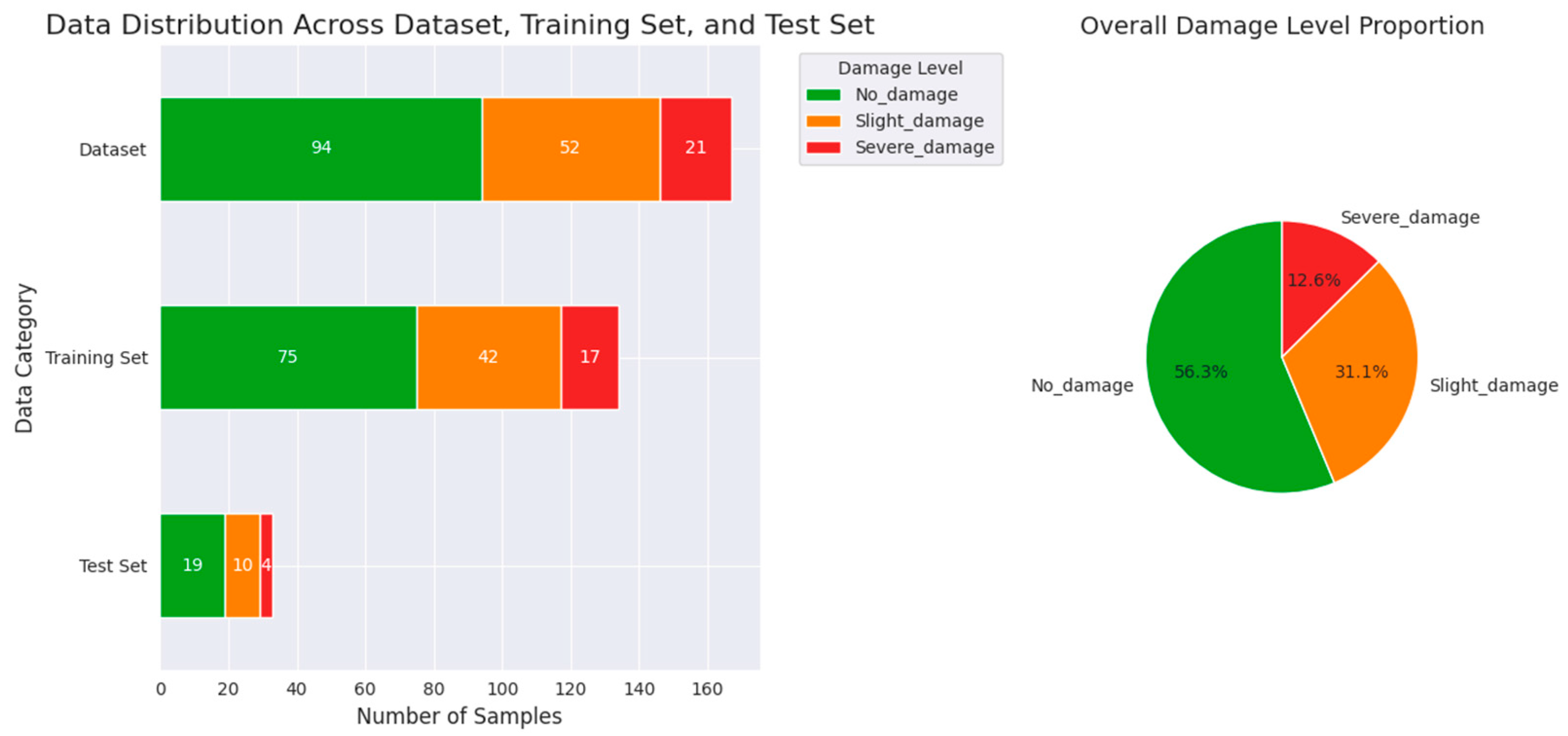
Furthermore, the sample size used in this study was limited to 167 sets. A larger sample size is needed, and future collaborations across different regions could enhance the model’s generalizability. Additional improvements could include expanding the dataset to include multiple mineral types, integrating time-series data to predict the long-term stability, and developing a real-time monitoring system embedded with the model.

Additionally, the model relies on high-quality mechanical parameter inputs. Insufficient on-site monitoring may affect the prediction accuracy. Future research should consider integrating finite element simulation with machine learning and developing a real-time parameter updating system to enhance the algorithm’s robustness and practicality.

6. Instance Validation

The Duimenshan section is located in the central part of the Mengzi Bainiuchang silver polymetallic mining area, extending from line 63 in the west to line 210 in the east, bounded by the F₃ fracture surface exposure line to the north, and near the Dajianpo to the south, covering an area of approximately 2.83 square kilometers. The region primarily features Middle and Lower Cambrian and Lower Devonian strata. The tectonic structure is predominantly characterized by northwest-oriented fractures and folds, with additional north/east and north/south-oriented structures, and notable magmatic activity. To validate the model constructed in this study, a statistical analysis of the mining section in the mined-out area was conducted. Statistical data as a sample were added to the test set of the RF prediction model, and the results are shown in

Table 6. Sample data of the goaf in the Duimenshan Mine.

Goaf	Shock Wave (m/s)	Compressive Strength (MPa)	Shear Strength (MPa)
1880-1	62.95	7.7	155.83
1850-1	64.92	8.1	153.59
1830-1	130.49	10.3	179.02
1800-1	212.87	13.1	202.68
1780-1	270.34	18.9	237.99

.

The RF prediction model predicted five mined-out areas, and the prediction results are shown in

Table 7. Comparison of the predicted results with the actual results.

Goaf	Prediction Results	Actual Results
1880-1	No damage	No damage
1850-1	No damage	No damage
1830-1	No damage	No damage
1800-1	Minor damage	Minor damage
1780-1	Serious damage	Serious damage

. In response, the mine staff promptly implemented precautionary measures to support the walls in advance, thereby reducing potential hazards. During the subsequent monitoring process, the predicted stability of the closed walls in the goaf was consistent with the actual site occurrence. Fortunately, there were no casualties, indicating that the prediction results exhibit strong consistency with the realities of the project.

7. Conclusions

In this study, the overall process of predicting the impact of shock waves on closed walls using the RF algorithm involves several of the following key steps: data preparation, model selection, hyperparameter optimization, model training, cross-validation, and performance evaluation. A total of 167 data samples, each containing three predetermined key input parameters, were collected to train and validate the RF machine learning model. Based on the introduction of four performance evaluation metrics, namely, the accuracy, precision, recall, and F1-score, within the experimental context of this study, we drew the following conclusions:

(1)

The analysis of the machine learning-based closed wall stability prediction model reveals that the random forest model demonstrates excellent predictive performance, achieving an accuracy of 94.6%. Following hyperparameter optimization through a grid search, the performance of the optimized random forest model is further enhanced, reaching an impressive accuracy of 95.9%. Compared to other algorithms, the method proposed in this paper does not exhibit a decrease in the prediction performance. Compared to the numerical model of Zhang et al. [19], the model presented in this paper improves the computational efficiency by approximately 40%.

(2)

Based on the model established in this study, the three parameters obtained from the experiments (the shock wave velocity, compressive strength, and shear strength) can effectively predict the stability of the closed walls in the project. To verify the reliability of the model, the machine learning prediction model was tested against data from 74 engineering examples and the Duimenshan mining area. The results indicate that the predicted stabilities of the closed walls are basically in line with the actual conditions, confirming that the RF prediction model exhibits superior performance and accuracy.

This high-performance prediction model provides a reliable and efficient tool for accurately assessing the impact of shock waves on closed walls, which is of great significance for theoretical research in the field of engineering geology. It fills a gap in the existing research to some extent by offering a more accurate and efficient prediction method for this specific engineering problem. This practical application not only validates the effectiveness of the model but also provides valuable guidance for real-world engineering projects, such as mine construction and underground engineering, where the stability of closed walls is crucial for ensuring safety and operational efficiency.

References

1. Chen, L.; Fan, S.; Zhao, C.; Zhang, L.; Cheng, Z. Calculation Method of Overburden Damage Height Based on Fracture Mechanics Analysis of Soft and Hard Rock Layers. Geofluids 2019, 2019, 3790264. [Google Scholar] [CrossRef]
2. Cai, M. Rockburst risk control and mitigation in deep mining. Deep Resour. Eng. 2024, 1, 100019. [Google Scholar] [CrossRef]
3. Lawal, A.I.; Adebayo, B.; Afeni, T.B.; Okewale, I.A.; Ajaka, E.O.; Amigun, J.O.; Akinbinu, V.A.; Apena, W.O. Soft Computing Applications for Optimum Rock Fragmentation: An Advanced Overview. Geotech. Geol. Eng. 2024, 42, 859–880. [Google Scholar] [CrossRef]
4. Wu, S.; Zhang, J.; Song, Z.; Fan, W.; Zhang, Y.; Dong, X.; Zhang, Y.; Kan, B.; Chen, Z.; Zhang, J.; et al. Review of the development status of rock burst disaster prevention system in China. J. Cent. South Univ. 2023, 30, 3763–3789. [Google Scholar] [CrossRef]
5. Badshah, E.; Naseer, A.; Ashraf, M.; Ahmad, T. Response of masonry systems against blast loading. Def. Technol. 2021, 17, 1326–1337. [Google Scholar] [CrossRef]
6. Yuan, F. Discussion on dynamic response of structure under shock wave of gas/coal dust explosion. Coal Mine Mach. 2017, 38, 65–67. [Google Scholar]
7. Zhao, Y.; Yan, X.; Zhang, Y. Damage Analysis of 3D Masonry Structures under Explosion Shock Waves Based on the CDEM. KSCE J. Civ. Eng. 2024, 28, 5781–5792. [Google Scholar] [CrossRef]
8. Qu, Z.; Wang, Y.; Zhou, X. Dynamic Laws and Numerical Simulation Study of Gas Explosion Shock Wave. Saf. Coal Mines 2013, 44, 1–5. [Google Scholar]
9. Qu, Z.; Li, J.; Wang, Y.; Zhou, X. Airflow Movement and Gas Migration Mechanism in Goaf Caving Area. Saf. Coal Mines 2013, 44, 9–13. [Google Scholar]
10. Qu, Z.; Zhou, X.; Wang, H.; Ma, H. Overpressure attenuation of shock wave during gas explosion. J. China Coal Soc. 2008, 33, 410–414. [Google Scholar]
11. Kallu, R.R. Effect of Roof Convergence on Stability of Underground Mine Seal Subjected to Explosion loading—Numerical Approach. In Proceedings of the 26th International Conference on Ground Control in Mining, Morgantown, WV, USA, 31 July–2 August 2007. [Google Scholar]
12. Cheng, J.; Ma, Z.; Wang, Z.; Ke, G.; Si, J.; Qin, Y.; Hu, X. Explosion Wave Pressure Distributions and Response Characteristics of Mine Seal Under the Complex Roadway Pattern. Min. Metall. Explor. 2023, 40, 1171–1186. [Google Scholar] [CrossRef]
13. Zhang, Q.; Qin, B.; Lin, D. Estimation of pressure distribution for shock wave through the bend of bend laneway. Saf. Sci. 2010, 48, 1263–1268. [Google Scholar]
14. Nima, M.; Hamzeh, G.; David, A.W.; Mohammad, M.; Shadfar, D.; Sina, R.; Alireza, S.; Amirafzal, K.S. A geomechanical approach to casing collapse prediction in oil and gas wells aided by machine learning. J. Pet. Sci. Eng. 2021, 196, 107811. [Google Scholar]
15. Salmi, E.F.; Ewan, J.S. A rock engineering system based abandoned mine instability assessment index with case studies for Waihi gold mine. Eng. Geol. 2022, 310, 106869. [Google Scholar] [CrossRef]
16. Luo, Y.; Xu, K.; Huang, J.; Li, X.; Liu, T.; Qu, D.; Chen, P. Impact analysis of pressure—Relief blasting on roadway stability in a deep mining area under high stress. Tunn. Undergr. Space Technol. 2021, 110, 103781. [Google Scholar] [CrossRef]
17. Wu, X.; Wang, S.; Gao, E.; Chang, L.; Ji, C.; Ma, S.; Li, T. Failure mechanism and stability control of surrounding rock in mining roadway with gentle slope and close distance. Eng. Fail. Anal. 2023, 152, 107489. [Google Scholar] [CrossRef]
18. Sun, S.; Jiang, Z.; Li, L.; Qiu, D. Model test and numerical verification of surrounding rock stability of super—Large—Span and variable—Section tunnels. Tunn. Undergr. Space Technol. 2024, 153, 106020. [Google Scholar] [CrossRef]
19. Zhang, Q.; Qin, B.; Lin, D. Estimation of pressure distribution for shock wave through the junction of branch gallery. Saf. Sci. 2013, 57, 214–222. [Google Scholar] [CrossRef]
20. Masi, F.; Stefanou, I.; Maffi-Berthier, V.; Vannucci, P. A Discrete Element Method based-approach for arched masonry structures under blast loads. Eng. Struct. 2020, 216, 110721. [Google Scholar] [CrossRef]
21. Edri, I.E.; Yankelevsky, D.Z. An analytical model for the out-of-plane response of URM walls to different lateral static loads. Eng. Struct. 2017, 136, 194–209. [Google Scholar] [CrossRef]
22. Dong, C.; Cheng, H. Study on Dynamic Impact Disaster Based on the Great Caving of Surrounding Rock in Goaf. Min. Res. Dev. 2016, 36, 38–40. [Google Scholar]
23. Geng, J. New Method of Computer Simulation for Shock Wave Created by Mined-out Area Roof Caving Based on Lattice-boltzmann. J. Anyang Inst. Technol. 2014, 13, 33–38. [Google Scholar]
24. Wang, M.; Luo, Z.; Yu, Q. Stability Prediction of Goaf Based on Stacking Model. Gold Sci. Technol. 2020, 28, 894–901. [Google Scholar]
25. Chen, J.; Tan, Y.; Huang, X.; Fu, J. Research on a Classification Method of Goaf Stability Based on CMS Measurement and the Cloud Matter–Element Model. Appl. Sci. 2024, 14, 3774. [Google Scholar] [CrossRef]
26. Zhao, B.; Zhao, Y.; Wang, J. New stability forecasting model for goaf slope based on the AHP–TOPSIS theory. Arab. J. Geosci. 2021, 14, 17. [Google Scholar] [CrossRef]
27. Zhao, X.; Liu, M.; Shi, F. Study of the prevention and control of large-scale impact disaster caused by roof caving with goaf overburden. Gold 2023, 44, 21–25. [Google Scholar]
28. Xing, P.; Song, X.; Fu, Y. Study on Similar Simulation of the Roof Strata Movement Laws of the Large Mining Height Workface in Shallow Coal Seam. Adv. Mater. Res. 2012, 450–451, 1318–1322. [Google Scholar] [CrossRef]
29. Xing, P.; Song, X.; Fu, Y. A Study on the Roof Fracture Mechanism of Large Cutting Height Workface in Shallow Thick Coal Seam. Adv. Mater. Res. 2011, 347–353, 183–188. [Google Scholar] [CrossRef]
30. Rodríguez, R.; Toraño, J.; Menéndez, M. Prediction of the airblast wave effects near a tunnel advanced by drilling and blasting. Tunn. Undergr. Space Technol. 2007, 22, 241–251. [Google Scholar] [CrossRef]
31. Janovsky, B.; Selesovsky, P.; Horkel, J.; Vejsa, L. Vented confined explosions in Stramberk experimental mine and AutoReaGas simulation. J. Loss Prev. Process Ind. 2006, 19, 280–287. [Google Scholar] [CrossRef]
32. Shen, Y.; Ning, J. Numerical simulation of the 2-D explosive field for the effect of protective wall’s shape. J. Beijing Inst. Technol. 2001, 10, 39–44. [Google Scholar]
33. Rajasekar, J.; Yaga, M.; Kim, H.D. Numerical prediction on the mitigation of shock wave using geometric barriers. J. Vis. 2023, 26, 83–96. [Google Scholar] [CrossRef]
34. Sha, C.; Wang, X.; Yang, H. Seepage Model of Water-Filled Goaf Based on Fluid-Solid Interaction. J. Northeastern Univ. (Nat. Sci.) 2023, 44, 551–557. [Google Scholar]
35. Xi, D.; Lu, H.; Zou, X.; Fu, Y.; Ni, H.; Li, B. Development of trenchless rehabilitation for underground pipelines from an academic perspective. Tunn. Undergr. Space Technol. 2024, 144, 105515. [Google Scholar] [CrossRef]
36. Jiang, X.; Zhang, M.; Song, Y.; Chen, H.; Huang, D.; Wang, D. Predicting ultrafast nonlinear dynamics in fiber optics by enhanced physics-informed neural network. J. Light. Technol. 2023, 42, 1381–1394. [Google Scholar] [CrossRef]
37. GB 6722-2014; Safety Regulations for Blasting. China Quality Standards Publishing & Media Co., Ltd: Beijing, China, 2014.
38. GB 50010-2010; Code for Design of Concrete Structures. China Architecture & Building Press: Beijing, China, 2010.
Figure 1. Shock wave formation mechanism (pump model). There are two types of the process in which the caving of the goaf roof compresses the air to form shock waves. (a) The rock mass of the overall collapse of the goaf roof and the rock wall of the goaf are equivalent to a piston and a cylinder respectively. This process is similar to the downward movement of the piston. The compressed air is rapidly discharged through the channel below the cylinder, forming an air shock wave. This is the pump model. (b) During the process of local collapse of the roof, part of the air flows around the rock blocks to the upper part of the goaf. This part of the air does not participate in the impact process. Another part of the compressed air, together with the impact airflow at the moment when the rock blocks land, forms an impact air wave. This is the spoiler model.
Applsci 15 02300 g001
Figure 2. Distribution of the input parameters. This figure illustrates the pairwise relationships between the following three input parameters in the dataset: the shock wave speed (SPEED), compressive strength (σbc), and shear strength (τ). The plots on the diagonal are kernel density estimations of each parameter’s distribution, while the off-diagonal scatter plots show the correlations between pairs of parameters. The different colors in the plot represent varying levels of damage (Damage): 1, 2, and 3. This figure allows for the observation of relationships between the parameters and their association with different levels of damage.
Applsci 15 02300 g002
Figure 3. Distribution of the input parameters. The figure consists of two subplots designed to illustrate the distribution of damage levels across different datasets. The horizontal stacked bar chart on the left shows the number of samples for each of the three damage levels—No_damage, Slight_damage, and Severe_damage—within the dataset (167 total samples), the training set (134 total samples), and the test set (33 total samples), respectively. The length of each bar represents the total number of samples, with different colors indicating the number of samples for each damage level. The pie chart on the right displays the proportion of each damage level within the entire dataset, clearly presenting the percentage of each damage level in the overall dataset.
Applsci 15 02300 g003
Figure 4. Correlation coefficient heatmap of the variables. This figure displays a correlation coefficient heatmap of four variables in the dataset: the shock wave speed (SPEED), compressive strength (σbc), shear strength (τ), and damage level (Damage). The color of each cell in the heatmap represents the strength of the correlation between the two corresponding variables, with redder colors indicating stronger positive correlations and bluer colors indicating stronger negative correlations. The number in each cell displays the specific correlation coefficient, which ranges from −1 to 1, where 1 represents perfect positive correlation, −1 represents perfect negative correlation, and 0 represents no linear correlation.
Applsci 15 02300 g004
Figure 5. Accuracy curves for each super hyperparameter. This figure consists of four subplots, each illustrating the impact of varying one hyperparameter of a random forest model on the model’s average accuracy. The four hyperparameters are as follows: the number of trees in the forest (n_estimators); the maximum depth of the tree (max_depth); the minimum number of samples required to be at a leaf node (min_samples_leaf); the minimum number of samples required to split an internal node (min_samples_split). In each subplot, the horizontal axis represents the value of the hyperparameter, and the vertical axis represents the corresponding average accuracy. The blue line in the graph connects the accuracy points corresponding to different hyperparameter values, forming an accuracy curve to observe the impact of hyperparameter changes on the model performance.
Applsci 15 02300 g005
Figure 6. Box plots of each hyperparameter versus the model accuracy. This figure consists of three box plots, each illustrating the impact of different values of three random forest model hyperparameters on the distribution of the model’s average accuracy. The three hyperparameters are as follows: maximum depth of the tree (max_depth); the minimum number of samples required to be at a leaf node (min_samples_leaf); the minimum number of samples required to split an internal node (min_samples_split). In each box plot, the horizontal axis represents the value of the hyperparameter, and the vertical axis represents the corresponding average accuracy. The box represents the middle 50% of the accuracy values in the dataset (i.e., the interquartile range), the horizontal line within the box represents the median, the whiskers represent the maximum and minimum values of the data (excluding outliers), and the circles represent outliers.
Applsci 15 02300 g006
Figure 7. Confusion matrix of the random forest model on the training set. This figure displays a confusion matrix for a classification model, used to evaluate the model’s predictive performance across different classes. The rows of the confusion matrix represent the predicted classes by the model (Prediction class), while the columns represent the true classes (True class). The value in each cell of the matrix indicates the number of samples where the model predicted a particular class, given the true class of the sample.
Applsci 15 02300 g007
Figure 8. Confusion matrix of the random forest model on the test set. This figure, similar to Figure 7, presents the confusion matrix ofTable a classification model on the test set.
Applsci 15 02300 g008