Research on Fitting and Denoising Subway Shield-Tunnel Cross-Section Point-Cloud Data Based on the Huber Loss Function

Abstract

The expansion of tunnel scale has led to a massive demand for inspections. Light Detection And Ranging (LiDAR) has been widely applied in tunnel structure inspections due to its fast data acquisition speed and strong environmental adaptability. However, raw tunnel point-cloud data contain noise point clouds, such as non-structural facilities, which affect the detection of tunnel lining structures. Methods such as point-cloud filtering and machine learning have been applied to tunnel point-cloud denoising, but these methods usually require a lot of manual data preprocessing. In order to directly denoise the tunnel point cloud without preprocessing, this study proposes a comprehensive processing method for cross-section fitting and point-cloud denoising in subway shield tunnels based on the Huber loss function. The proposed method is compared with classical fitting denoising methods such as the least-squares method and random sample consensus (RANSAC). This study is experimentally verified with 40 m long shield-tunnel point-cloud data. Experimental results show that the method proposed in this study can more accurately fit the geometric parameters of the tunnel lining structure and denoise the point-cloud data, achieving a better denoising effect. Meanwhile, since coordinate system transformations are required during the point-cloud denoising process to handle the data, manual rotations of the coordinate system can introduce errors. This study simultaneously combines the Huber loss function with principal component analysis (PCA) and proposes a three-dimensional spatial coordinate system transformation method for tunnel point-cloud data based on the characteristics of data distribution.

1. Introduction

The growth in transportation demand and the expanded utilization of underground space have driven the rapid development of tunnel engineering, leading to the continuous expansion of tunnel scale worldwide [1]. Shield tunnels have become the predominant form in most urban subway systems due to their advantages, such as construction convenience [2]. However, the growth in tunnel scale has also brought about a series of issues. Due to factors such as the aging of tunnel structures and the mechanical effects of the surrounding soil on the tunnel, structural deformation and damage inevitably occur. RThese issues ultimately affect the load-bearing capacity of the tunnel structure and pose safety hazards.

At the same time, defects such as cracks, spalling, and lining water leakage are widely present in operational tunnels [3,4], which also impact the load-bearing performance of tunnel structures. Therefore, structural inspections of tunnels play a crucial role in tunnel operations [5].

Traditional tunnel inspections primarily rely on manual methods, using tools such as measuring tapes, rangefinders, ground-penetrating radars, and total stations to collect data [6,7,8]. However, these measurement methods require significant time, manpower, and material resources during preparation and measurement. Additionally, the measurement accuracy for tunnel deformation is greatly affected by factors such as human intervention and the arrangement of measurement points [9]. Therefore, there is a significant demand for rapid and high-accuracy detection methods for structural deformation in the field of tunnel inspections.

Light Detection And Ranging (LiDAR) has been widely applied in structural inspections due to its advantages, such as non-contact measurement and fast data acquisition. Laser scanning systems, including mobile laser scanning systems and tripod-based laser scanning systems, are also increasingly being utilized in tunnel inspections [10,11].

However, laser scanning systems acquire surface point-cloud data of tunnels during the scanning process, and these raw point-cloud data contain a large number of non-structural facilities, such as pipelines and maintenance walkways. While these non-structural facilities have relatively little impact on the mechanical performance of the shield tunnel itself, the effectiveness of removing non-structural facility point clouds significantly affects the health inspection of the tunnel lining structure [12].

Numerous researchers have conducted extensive studies on point-cloud denoising, integrating various computer science theories into the denoising process. This has led to the development of a range of point-cloud processing techniques, including filter-based point-cloud denoising, optimization-based point-cloud denoising, and machine learning-based point-cloud denoising [13,14,15].

Filter-based point-cloud denoising primarily originates from the concept of filters in signal processing, where appropriately designed filters are used to remove unwanted noise components. This method typically smooths the data directly through weighted averaging or similar operations, eliminating noise while striving to preserve the characteristics of the original signal. For example, Wen et al. [16]. considered the impact of three parameters—number of nearest neighbor points (N), Euclidean distance weight, and normal vector direction weight—on denoising performance and applied bilateral filtering to denoise point-cloud data in autonomous driving scenarios. Similarly, Wang et al. [17]. denoised forest point-cloud data using statistical filtering, effectively segmenting ground point-cloud data and individual tree point-cloud data.

In addition, filters such as statistical outlier removal (SOR) [18], geometry-based filtering [19,20], and radius filtering [21] have also been applied to point-cloud denoising in various scenarios. Filter-based point-cloud denoising achieves good results when targeting specific point-cloud distributions. In filter-based point-cloud denoising methods for tunnel structures, filtering techniques such as cloth simulation filtering (CSF) [22] and wavelet transform [23] have achieved promising results.

Optimization-based point-cloud denoising methods formulate the denoising process as an optimization problem. By defining objective functions based on geometric properties and noise distributions, these methods seek a denoised point cloud that best fits the objective function derived from the input noisy point cloud.

Fitting methods, represented by the least-squares method [24], have achieved notable results in point-cloud denoising. This approach introduces locally approximated surface polynomials to adjust point set density, enabling the smooth reconstruction of complex surfaces while minimizing geometric errors. The least-squares method and its improved variants have also been widely applied in the denoising of point-cloud data [25,26,27,28]. Meanwhile, the least-squares method, combined with other denoising techniques such as outlier filtering [29] and local kernel regression (LKR) [30], has also been applied to point-cloud data denoising. In addition to the least-squares method, other fitting optimization techniques, such as local optimal projection (LOP) [31], weighted local optimal projection (WLOP) [32], and moving robust principal component analysis (MRPCA) [33], have also been widely applied.

Some of the aforementioned point-cloud denoising techniques have also been applied to the processing of tunnel-structure point-cloud data. Bao, Yan et al. [34] conducted research on denoising tunnel cross-sectional point clouds by leveraging the geometric features and intensity information of the point-cloud data. Their method effectively removes most noise points in the tunnel point cloud, thereby improving data quality and accuracy. However, because this method requires manually transforming the coordinate system and extracting the cross-section based on the point cloud’s geometric and intensity features, the denoising accuracy is significantly affected by factors such as equipment, environment, and the precision of manual data preprocessing. Consequently, its robustness under complex tunnel conditions is relatively poor.

Since the tunnel cross-sectional structure exhibits minimal variation along the tunnel’s mileage, some scholars have extracted tunnel cross-sections along the mileage direction based on this structural characteristic [35] and performed denoising on individual cross-section point clouds. Moreover, Soohee Han et al. [36] projected the three-dimensional point cloud onto a two-dimensional plane and extracted the tunnel axis by obtaining the planar skeleton, thereby achieving tunnel cross-section extraction.

In addition, some researchers employ ellipse-fitting methods to model the boundary lines of tunnel point clouds and, based on the fitting results, remove outliers to complete both the denoising of tunnel cross-sectional point clouds and the extraction of the cross-section. Among various ellipse-fitting methods, the least-squares method [37,38,39,40] is widely used. The least-squares method can effectively fit and denoise tunnel point clouds that contain relatively few noise points and where the noise causes only minimal dispersion of the fitted curve. However, some tunnel point clouds contain a significant amount of discrete noise, such as those generated by tunnel pipelines, making it difficult for the least-squares method to perform effective fitting and denoising.

In order to improve the robustness of the fitting method against noise, some researchers have employed RANSAC [41,42,43] to fit tunnel cross-sectional curves. RANSAC is highly robust method capable of extracting valid data even in the presence of a large amount of noise and outliers, making it suitable for complex point-cloud distributions with unevenly distributed noise or numerous outliers. However, the selection of parameters for this method (such as the inlier threshold and the number of iterations) relies on experience, and the tuning process is quite cumbersome. Moreover, because this method is based on random sampling, the ellipse-fitting results obtained with RANSAC tend to be unstable and lack repeatability. In addition, B-spline curves [44] have also been applied to the curve fitting of tunnel cross-sectional point clouds. This method can generate smooth, continuous curves with excellent local control, making it suitable for describing complex tunnel cross-sectional shapes. However, it is sensitive to the selection of initial control points and parameter settings, and inappropriate settings may lead to fitting bias.

Machine learning-based point-cloud denoising does not rely on manually defined filters or objective functions. Instead, it denoises through a data-driven approach, leveraging the powerful computational capabilities of computers to uncover the inherent patterns and features within the data. Machine learning primarily includes two types: supervised learning and unsupervised learning.

In the field of point-cloud denoising, unsupervised learning denoising methods are often based on clustering techniques. These methods group similar data points into clusters and identify and remove outliers or noise points to achieve denoising. Density-based clustering algorithms such as DBSCAN [45]; PCA-based adaptive clustering [46]; the DTSCAN clustering method based on Delaunay triangulation and the DBSCAN mechanism [47]; clustering based on spatial distance, normal similarity, and logarithmic Euclidean Riemannian metrics [48]; and K-means clustering based on local statistical features of point clouds [49] have been applied to point-cloud denoising.

These methods have achieved good denoising results for point-cloud data with distinct geometric distribution features. These unsupervised learning models typically do not require explicit labels. Instead, they learn the inherent features of the data by identifying structures, patterns, or correlations within the data.

In contrast, supervised learning involves learning from labeled training data to predict outcomes for new, unseen data. In the field of point-cloud denoising, supervised learning-based denoising is often achieved using neural networks. Network architectures such as PointNet and convolutional neural networks (CNNs) have been applied to point-cloud denoising.

The PointNet [50] and PointNet++ [51] architectures, which can directly process point-cloud data, have opened new directions in the field of 3D data processing and have driven the development of point-cloud processing networks. Improved versions of the PointNet network, such as PointCleanNet [52], which focuses on the fusion of local and global features of point clouds, and PCPNet [53], which emphasizes the estimation of local geometric features like normal vectors and curvature, have demonstrated good performance in point-cloud denoising tasks.

PointNet has relatively weak local feature extraction capabilities and lacks spatial structure awareness of point-cloud data. To address this, some researchers have employed improved convolutional neural networks (CNNs) for point-cloud denoising tasks [54,55,56,57]. For existing convolutional neural networks (CNNs), the unstructured and sparse nature of point-cloud data does not perfectly match the input data requirements of CNNs. Therefore, the use of CNNs for point-cloud denoising still has room for improvement. In machine learning-based point-cloud denoising, DBSCAN clustering [58] has been applied to tunnel point-cloud denoising.

In the aforementioned research on point-cloud denoising, various models of laser scanning devices have been applied for point-cloud acquisition. For instance, the Faro X130, which excels in high-precision detail capture, features a scan angular resolution of 0.036° and a beam divergence of 0.19 mrad, a measuring range of 0.6 m to 130 m, and a single measurement error of ±2 mm; a single scan can generate a high-density point cloud containing approximately 1371 million points. Additionally, the Robosense Helios 1615 laser scanner, known for its fast measurement speed and suitability for mobile mapping and large-scale three-dimensional laser scanning, employs a 32-line scanning mechanism, offers a 360° horizontal field of view and a 70° vertical field of view (covering −55° to +15°), and can achieve a point-cloud acquisition rate of 576,000 pts/s in single-return mode.

In addition, the Optech LYNX Mobile Mapper, which is suitable for engineering surveys and large-scale infrastructure measurements (such as tunnels), features a maximum measuring range of 200 m, a range precision of 8 mm, and a range accuracy of ±10 mm (1σ). This device has a laser measurement rate of 75–500 kHz (with multiple measurements possible per laser pulse), a scanning frequency of 80–200 Hz, uses a 1550 nm (near-infrared) laser, and offers a full 360° scanning field of view. Besides laser scanning devices, other data acquisition devices, such as the Intel RealSense D435i, are also used for data collection tasks. The Intel RealSense D435i is a measurement device that generates depth images based on infrared stereo vision and related technologies. It features an RGB frame resolution of 1920 × 1080 and a field of view of approximately 69° × 42°. This device is capable of capturing both RGB and depth information simultaneously. Together, these devices provide a reliable data foundation for the aforementioned denoising methods.

However, in point-cloud denoising methods for tunnel data, filter-based denoising techniques often focus on the distribution of individual point clouds and tend to have poor robustness when dealing with complex point-cloud distributions. Machine learning-based point-cloud denoising methods, represented by clustering and neural networks, often involve complex parameter tuning or require large amounts of data collection and labeling. As a result, these methods typically have long preparation periods and substantial workloads. Optimization-based denoising methods, such as point-cloud fitting, often require manual data preprocessing. The quality of the preprocessing directly affects the ellipse-fitting results, which in turn impacts the denoising performance. However, for large-scale point-cloud data in practical inspection tasks, performing manual preprocessing on all the data would consume substantial resources.

Therefore, this study proposes an ellipse-fitting denoising method based on the Huber loss function. This method achieves good fitting results and effectively denoises tunnel-lining-structure point-cloud data without the need for preprocessing. Additionally, it offers good computational efficiency.

2. Methods

The process of ellipse-fitting and point-cloud data denoising for subway shield-tunnel sections based on the Huber loss function is shown in Figure 1. Raw point-cloud data of the subway tunnel are obtained through a mobile laser scanning system. The raw point-cloud data undergo principal component analysis (PCA) to determine the principal component direction of the point-cloud data and use the Huber loss function to fit the cross-section’s symmetry axis. Based on the principal component direction and the fitted symmetry axis, the spatial coordinate system of the point-cloud data is transformed. This ensures that the mileage direction (tunnel axis direction) of the tunnel point cloud aligns parallel to the Cartesian coordinate system’s z-axis, the symmetry axis of the tunnel cross-section aligns parallel to the y-axis, and the x-axis remains orthogonal.

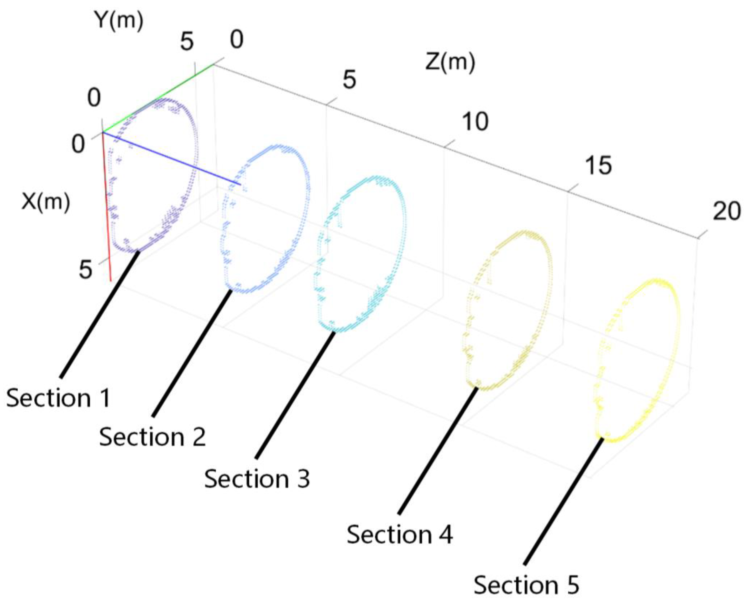
After transforming the coordinate system, tunnel point-cloud data are extracted along the z-axis direction at fixed distances to obtain cross-sectional point-cloud data. For each individual cross-section point cloud, the Huber loss function is used to fit an ellipse equation. The original point cloud is then projected onto the fitted ellipse by calculating the radial shortest distance, resulting in the denoised point cloud.

Finally, evaluation metrics are derived by calculating the differences in radial distance between before and after projection. These metrics include mean squared error (MSE), root-mean-squared error (RMSE), and mean absolute error (MAE), which are used to comprehensively assess the effectiveness of tunnel point-cloud data denoising.

2.1. PCA-Based Point-Cloud Data Coordinate System Transformation

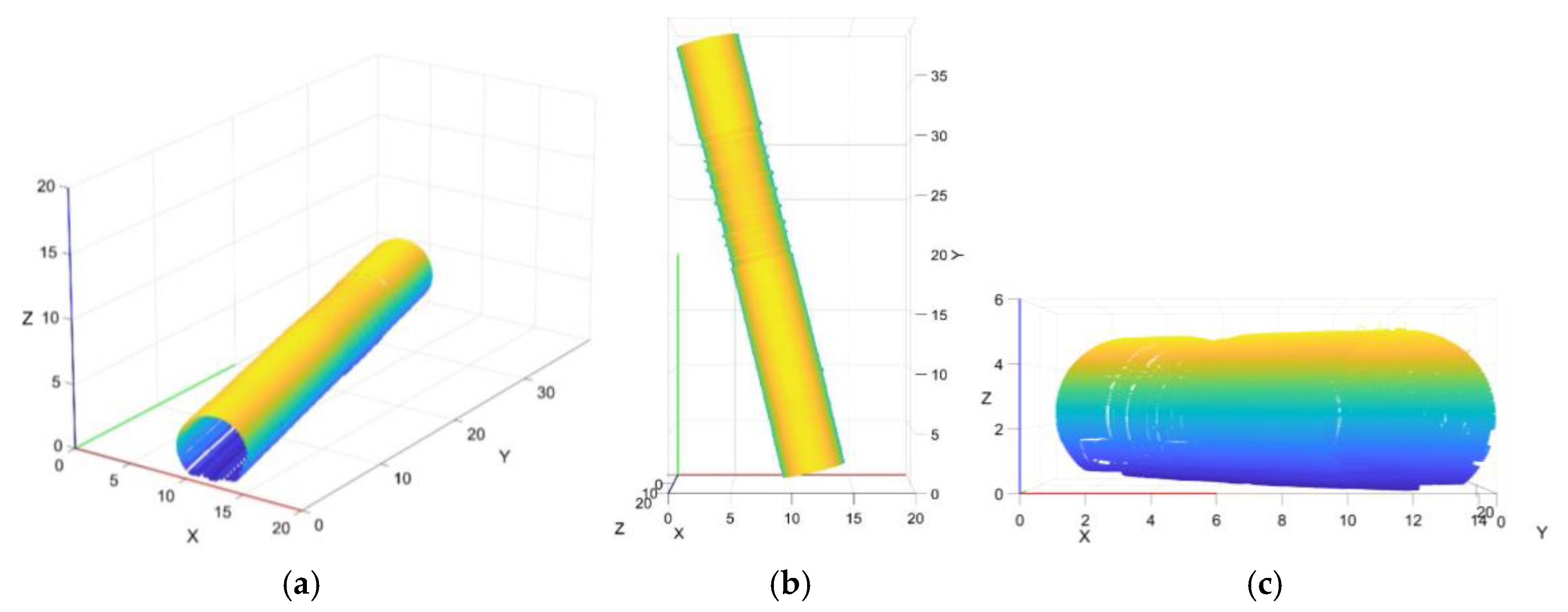
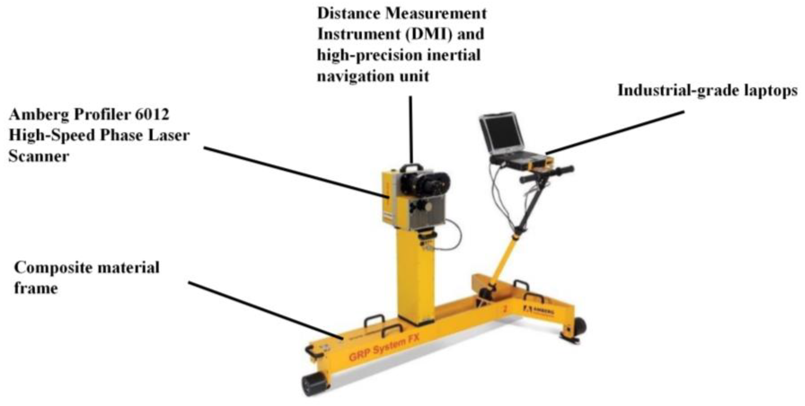
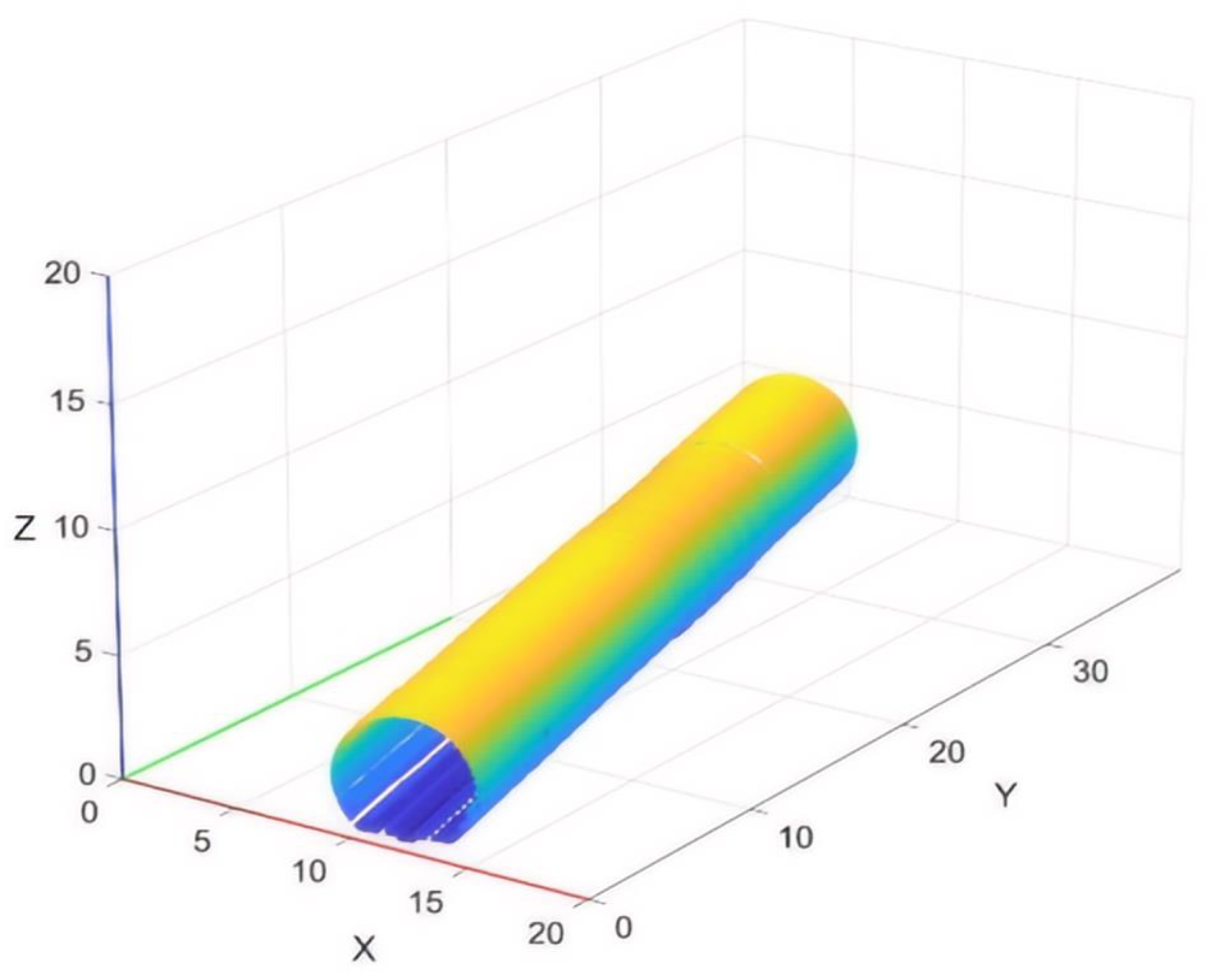
Due to significant variations in the actual tunnel alignment direction caused by engineering requirements, geological conditions, and other factors, the principal feature direction of the tunnel point-cloud data scanned by the laser scanning system is not orthogonal to the XYZ axes of the Cartesian coordinate system. This study selected the Amberg Clearance GRP 5000—Profiler 6012 model mobile 3D laser scanner to collect data, which is a high-precision measurement system designed for tunnel and rail infrastructure inspection. The laser scanning system quickly advances along the tunnel axis to achieve continuous tunnel point-cloud data collection. The actual collected tunnel point-cloud data are shown in Figure 2. Since the tunnel point cloud is a three-dimensional graphic, a single color cannot display the three-dimensional graphic. This study uses a color threshold that is evenly distributed along the point-cloud data to display the three-dimensional point-cloud graphics. The color threshold in the figure has no actual geometric or physical meaning.

However, during point-cloud data processing, coordinate system transformation is often involved. To achieve better computational results and facilitate calculations, this study proposes a PCA-based tunnel point-cloud coordinate system transformation method. This method rotates the principal feature direction of the original point-cloud data to align with the z-axis of the Cartesian coordinate system. The results show that this method effectively completes the tunnel point-cloud coordinate system transformation and reduces the errors introduced by manual operations.

PCA is a commonly used data feature extraction method that represents the main variation trends of the data by finding the direction with the largest variance (i.e., the principal components). A larger variance indicates that the differences in the data are more pronounced. PCA was first proposed by Karl Pearson [59] in 1901. It uses linear combinations to reduce the dimensionality of high-dimensional data to process multivariate data, revealing the correlation between variables and the inherent structure of the data. Later, it was further developed and improved by Harold Hotelling [60] and named “principal component analysis”. This method has been widely used in the field of data statistical analysis. Li, D. [61] et al. successfully extracted the principal axis direction of the turbine-blade point cloud with the help of PCA, proving the effectiveness of the PCA method in extracting the principal component direction of point-cloud data. Based on the above PCA principles and references, this study improves the PCA formula for tunnel point-cloud data processing and applies it to tunnel point-cloud coordinate system transformation. For tunnel point-cloud data with a narrow distribution, this method can effectively extract the principal component direction.

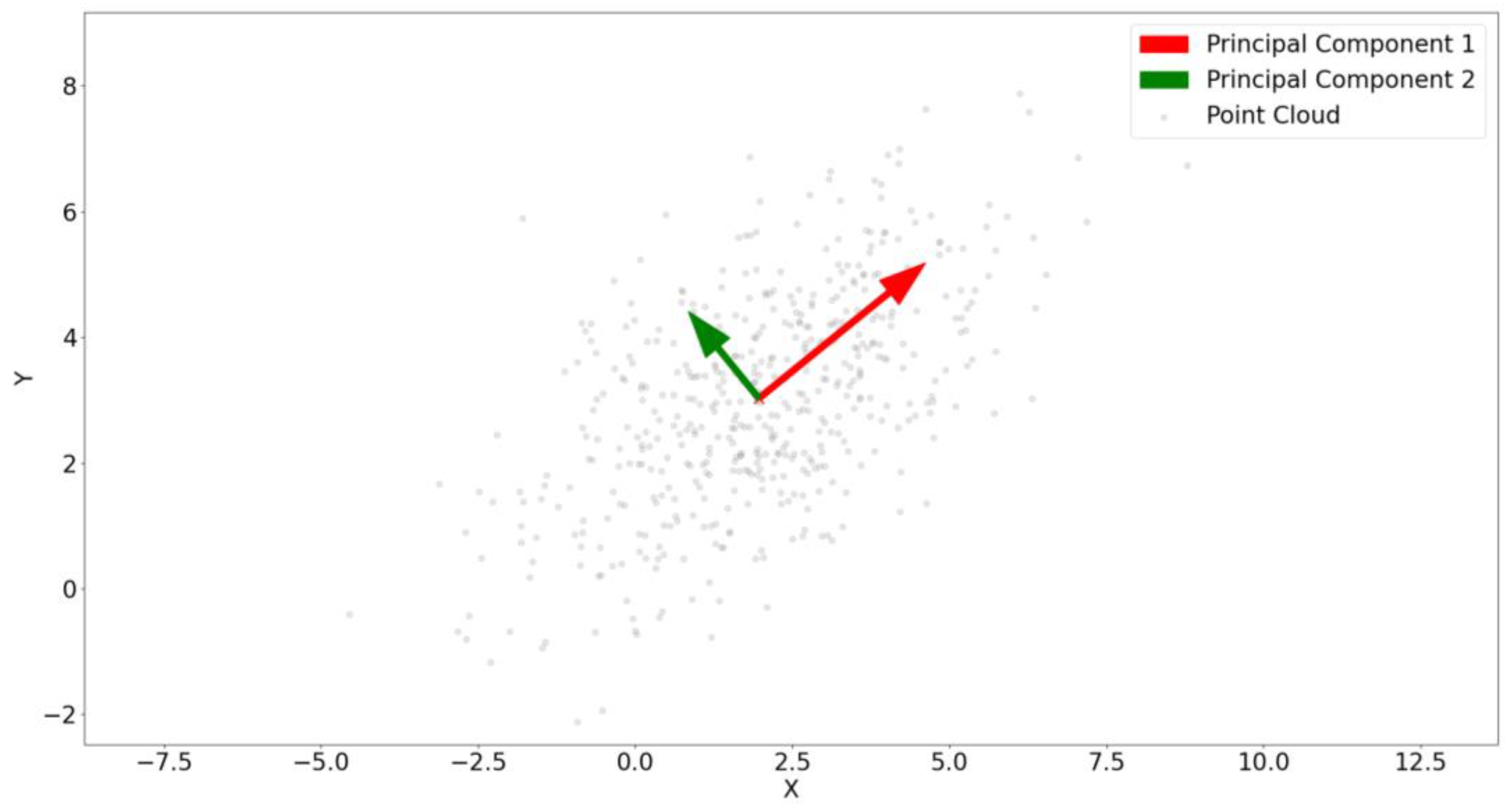
Since the actual amount of tunnel point-cloud data is huge, usually counted in millions, it is difficult to directly use tunnel point-cloud data to show the principal component direction of the tunnel point cloud. In order to better demonstrate the PCA principle, this paper uses the sample point-cloud data generated by Python to visualize the PCA principle, as shown in Figure 3. The two arrows in the figure represent the first and second principal component directions of the data. The gray dots are sample data generated by the program, representing the point-cloud data of the actual tunnel. The coordinate axes in the figure are for the quantitative display of point-cloud data and do not have actual units.

To reduce the errors introduced by manually selecting the tunnel axis direction, this study uses PCA to calculate the eigenvector of the direction with the maximum variance of the tunnel point cloud (the first principal component direction) to represent the tunnel point cloud’s axis direction. Based on this, the tunnel point cloud is rotated, as shown in Figure 4.

For the original tunnel point-cloud dataset $X={\left\{x_i\right\}}_{i=1}^N$, where each point in the dataset has coordinates $\left(x_i,y_i{,z}_i\right)$, in order to eliminate the effect of the data’s position (i.e., the offset) in the coordinate space on the data’s feature vector (i.e., the principal component direction), the mean of the point-cloud data must be calculated according to Equation (1), and then all points in the point-cloud dataset are centered by subtracting the mean, as shown in Equation (2).

$$\overline{x}={\displaystyle \frac{1}{N}}\sum _{i=1}^N{x}_i$$

(1)

$$X_{centered}={\left\{x_i-\overline{x}\right\}}_{i=1}^N$$

(2)

The original tunnel point-cloud data are centered by subtracting the mean, resulting in the centered tunnel point-cloud dataset $X_{centered}$. The covariance matrix $C$ of $X_{centered}$ is then calculated according to Equation (3). The covariance matrix $C$ undergoes eigenvalue decomposition, as shown in Equation (4). The principal component corresponds to the largest eigenvalue ${\lambda }_1$, and the eigenvector $v_1$ associated with ${\lambda }_1$ represents the axis direction of the tunnel point-cloud data.

$$C={\displaystyle \frac{1}{N}}\sum _{i=1}^N(x_i-\overline{x}){\left(x_i-\overline{x}\right)}^T$$

(3)

$${Cv}_i{=\lambda }_i{v}_i$$

(4)

In the equation, ${\lambda }_i$ represents the i-th eigenvalue of the covariance matrix, and $v_i$ is the eigenvector corresponding to ${\lambda }_i$. The eigenvalues are solved in descending order, such that ${\lambda }_1>{\lambda }_2>{\lambda }_3$.

To align the obtained principal axis direction of the point cloud with the Z-axis direction, the rotation axis r and the rotation angle $\theta$ need to be calculated. Based on these, the rotation matrix R is computed. The rotation vector r is calculated as shown in Equation (5), and the normalized rotation vector $r_{norm}$ is calculated as shown in Equation (6), which represents the direction of rotation. The x, y, and z axes represent the corresponding rotation vectors $r_x$, $r_y$, $r_z$. The rotation angle $\theta$ can be computed using the dot product between the principal axis and the Z-axis, as shown in Equation (7).

$$r{=v}_1\times z$$

(5)

$$r_{norm}={\displaystyle \frac{r}{‖r‖}}$$

(6)

$$\theta =arccos\left({\displaystyle \frac{v_1\times z}{‖v_1‖\times ‖z‖}}\right)$$

(7)

In the equation, $‖v_1‖$ and $‖z‖$ represent the magnitudes of the unit vectors along the principal axis and the z-axis, respectively.

In three-dimensional space, the rotation matrix can be generated using axis–angle representation. For any point $\left(x_i,y_i{,z}_i\right)$ in space, the coordinates of the rotated point can be directly obtained by multiplying it with the rotation matrix $R$. Given a rotation vector $r_{norm}$ and a rotation angle $\theta$, the rotation matrix $R$ can be generated using Rodrigues’ equation, as shown in Equation (8). The skew–symmetric matrix is defined in Equation (9).

$$R=I+\sin \theta K+\left(1-\cos \theta \right)K^2$$

(8)

$$K=\left[\begin{array}{ccc}0& {-r}_z& r_y\\ r_z& 0& {-r}_x\\ {-r}_y& r_x& 0\end{array}\right]$$

(9)

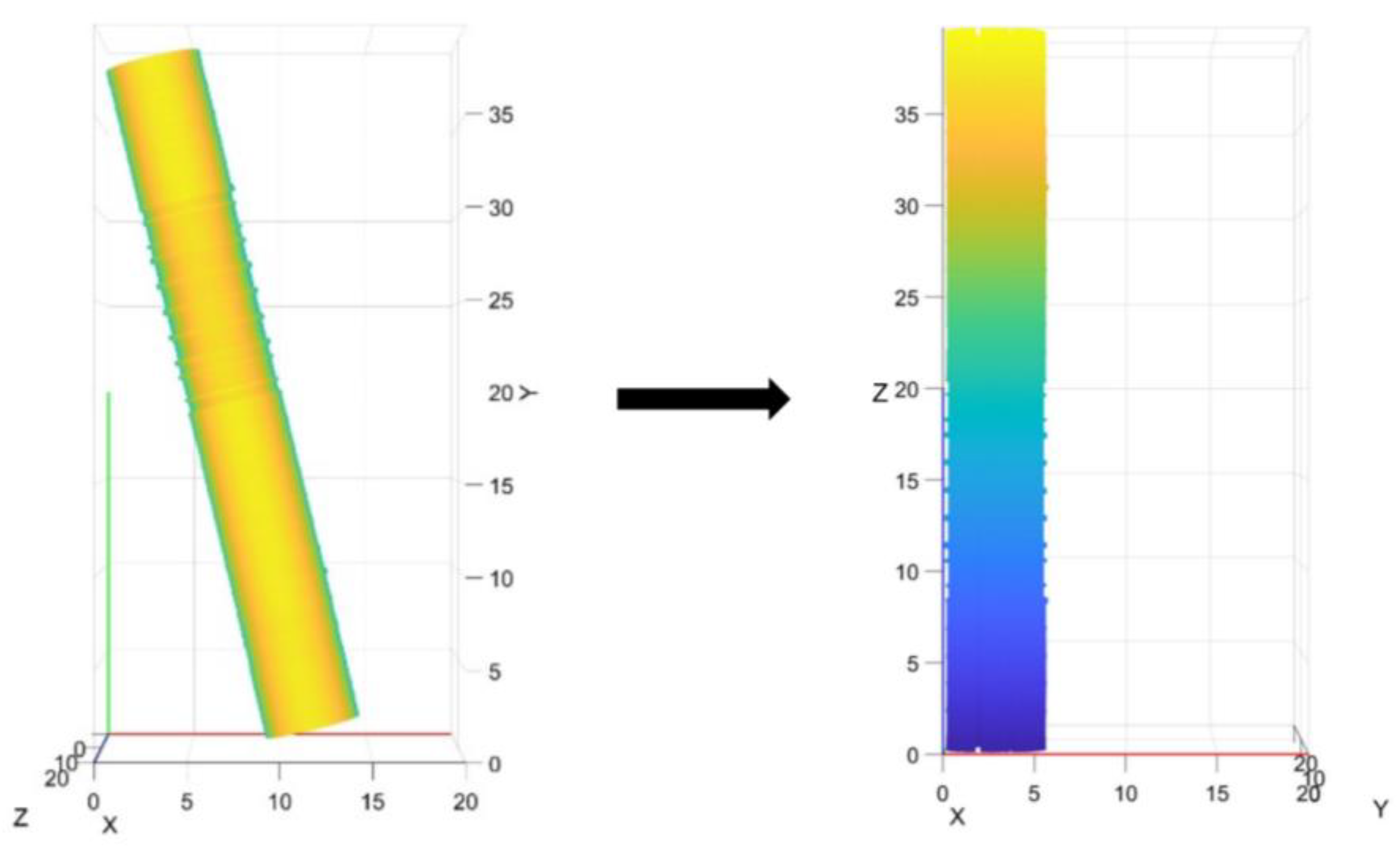
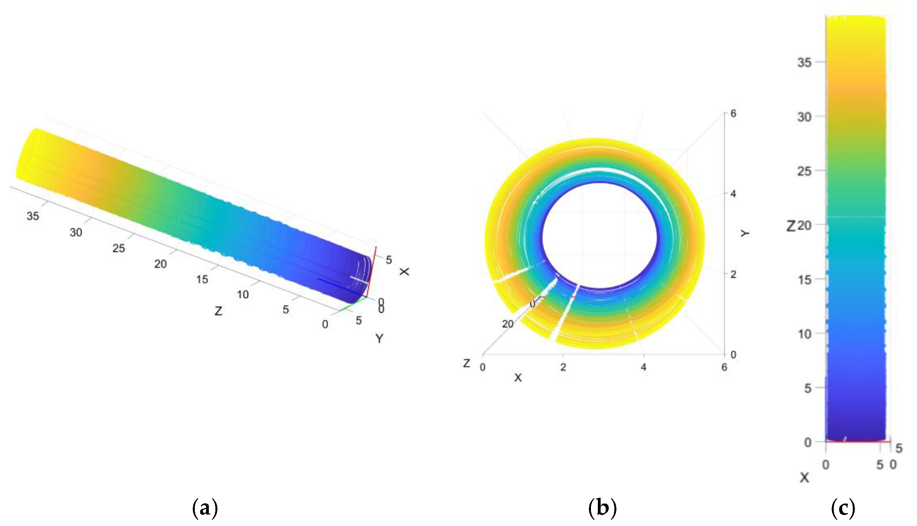
The original point cloud is rotated along the tunnel axis, and the entire-tunnel point cloud is rotated to align with the z-axis direction, as shown in Figure 5.

2.2. Point-Cloud Coordinate Transformation and Section Fitting Denoising Based on Huber Loss Function

The PCA-based point-cloud coordinate transformation can align the tunnel point cloud’s main axis direction with the target axis (Z-axis direction), so that the tunnel section becomes parallel to the XY plane of the Cartesian coordinate system. However, for the tunnel point cloud after coordinate transformation, the actual tunnel section is not orthogonal to the XY plane, and the point cloud contains a large amount of noise points generated by tunnel ancillary facilities. To address this issue, this study proposes a method for tunnel-section coordinate system transformation and section fitting denoising based on the Huber loss function.

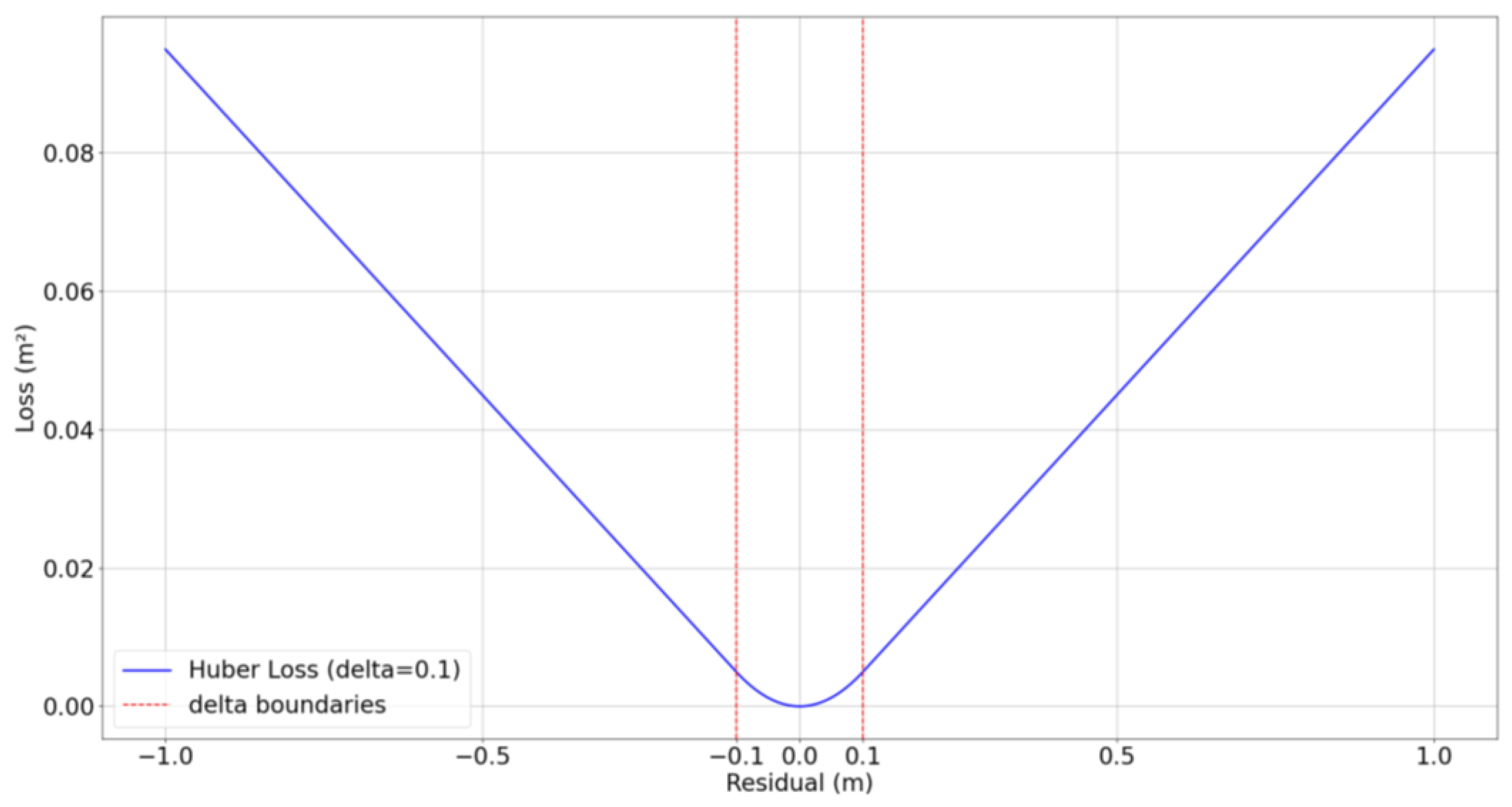
The Huber loss function was proposed by statistician Peter J. Huber in [62]. It combines the square error (for small deviations) and the linear error (for large deviations), as shown in Equation (10). Therefore, this fitting method is more robust to outliers. Based on the principle of the Huber loss function and some vector algebra and Euclidean geometry principles, this study proposes the following method and formula.

The principle of the Huber loss function is illustrated in Figure 6. The objective of fitting using the Huber loss is to minimize the loss between the fitting function and all the points, as shown in Equation (11). In this study, the fitting result using the Huber loss function is a circular equation. This equation describes the distribution and geometric parameters of the tunnel cross-sectional point cloud, laying the foundation for subsequent point-cloud coordinate transformation and denoising. In this circular equation, the circle’s center is defined as $\left(h_0,k_0\right)$, and the radius is $R_0$. By minimizing this loss function, the circle’s center $\left(h_0,k_0\right)$ and radius $R_0$ can be determined.

In this study, the geometric parameters of the tunnel cross-section are fitted using the Huber loss function $L_{\delta }\left(r_i\right)$, which serves as the basis for coordinate system transformation and point-cloud denoising.

$$L_{\delta }\left(r_i\right)=\left\{\begin{array}{c}0.5·r_i^2 if\left|r_i\right|\le \delta \\ \delta ·\left(\left|r_i\right|-0.5·\delta \right) if\left|r_i\right|>\delta \end{array}\right.$$

(10)

$${min}_{h,k,r}={\sum }_{i=1}^N {\omega }_i{L}_{\delta }\left(r_i\right)$$

(11)

In the Equation (10), $\delta$ is a parameter used to control the transition of the function from squared residuals to linear residuals. When the absolute value of the residual is less than or equal to $\delta$, the loss function behaves as squared residuals, making the loss function smoother for small residuals. When the absolute value of the residual exceeds $\delta$, the loss function transitions to a linear increase, reducing the influence of outliers on the fitting result. $\left|r_i\right|$ represents the absolute residual between the fitted value and the actual value. ${\omega }_i$ is the weight parameter, which controls the impact of the point-cloud data’s error on the total loss.

In Equation (11), the subscripts h, k, and r represent the parameters optimized in the minimization process, which represent the x-coordinate of the circle center, the y-coordinate of the circle center, and the radius of the circle, respectively. The algorithm continuously adjusts these three parameters to minimize the Huber loss function, and the obtained equation is the circle equation with the best fitting effect for the tunnel point-cloud section.

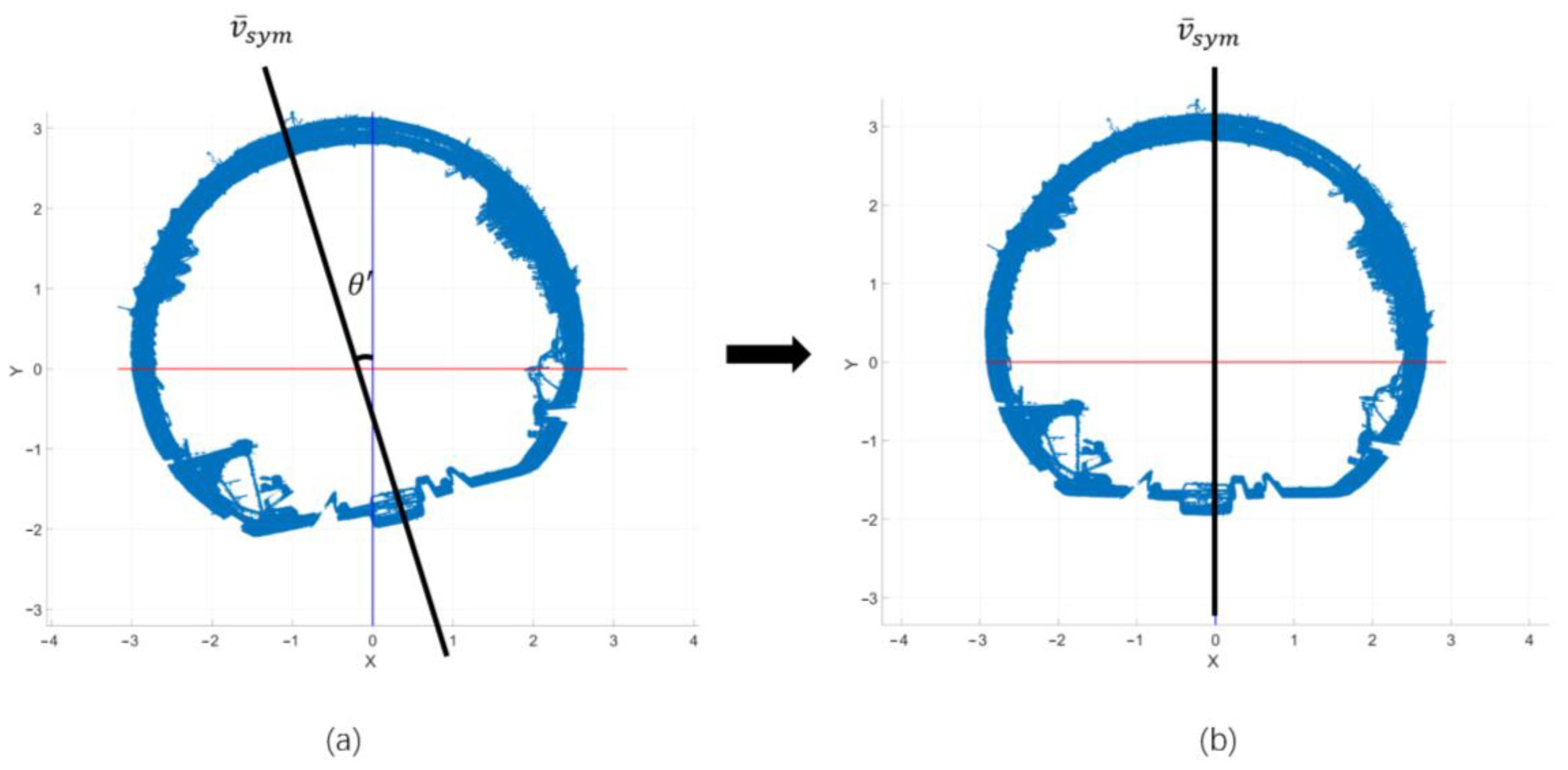
The Huber loss function can fit the center, axis of symmetry, and other geometric information of the tunnel cross-section. Using this geometric information, the axis of symmetry direction $v_{sym}$ for each cross-sectional point set $X_{seg}$ can be computed. By calculating the average axis of symmetry direction ${\overline{v}}_{sym}$ for all cross-sections and the angle ${\theta }^{\mathrm{\prime }}$ between it and the XY plane axis, the point-cloud data can be rotated around the Z-axis ${\theta }^{\mathrm{\prime }}$, thus obtaining the tunnel point cloud that is orthogonal to the XY plane, as shown in Figure 7.

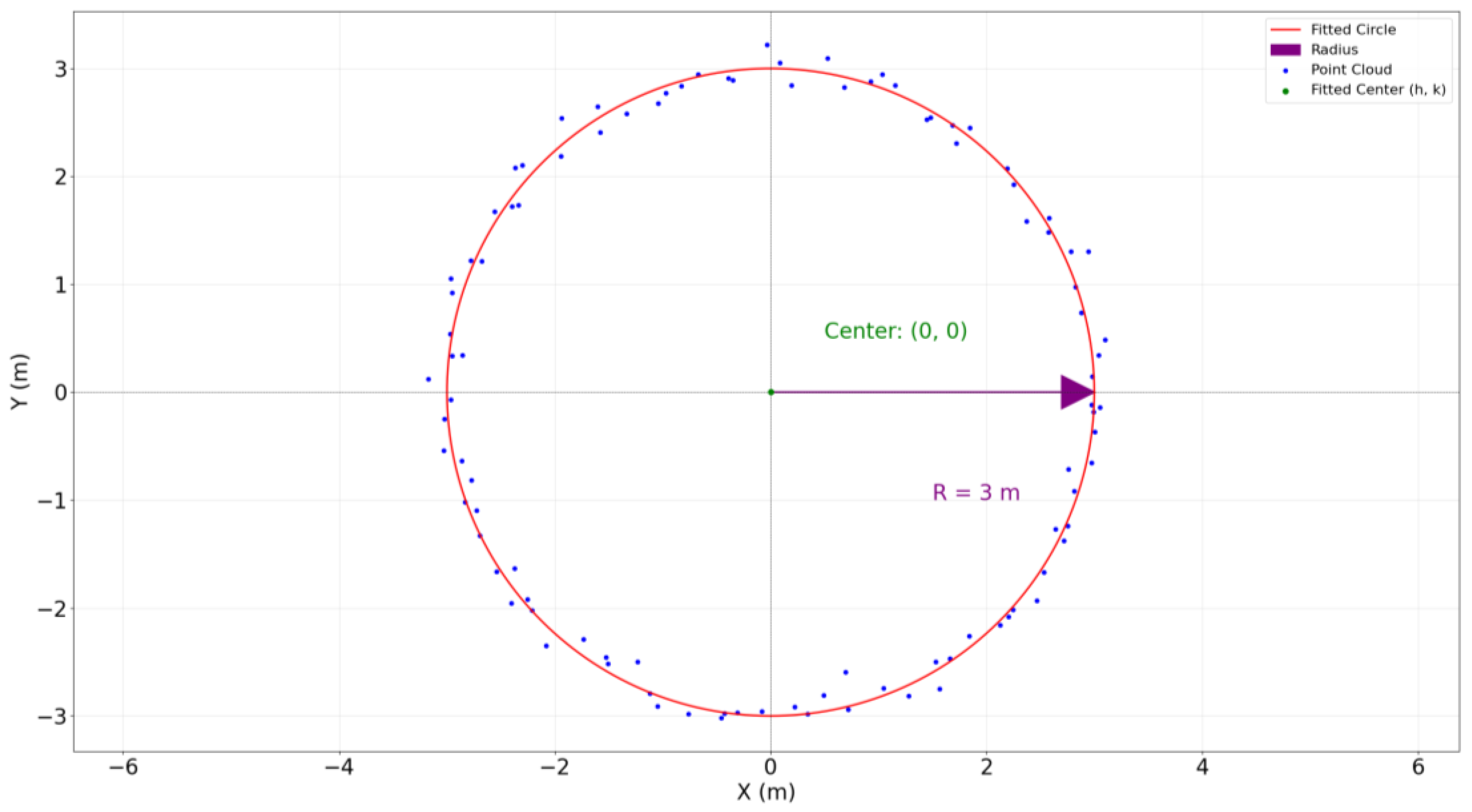
For a single tunnel cross-section point cloud, in order to improve computational efficiency and make the point cloud easier to fit, a circular model with only two parameters is selected for the fitting, as shown in Equation (12). In this equation, $\left(h,k\right)$ represents the center of the fitted circle, and $R$ is the radius of the fitted circle. The goal is to minimize the residuals between the fitting function and all points, i.e., to make all points fall as close as possible to the fitted circle, as illustrated in Figure 8.

$$r_i=\sqrt{{\left(x_i-h\right)}^2+{\left(y_i-k\right)}^2}-R$$

(12)

For the fitted circle center $\left(h_0,k_0\right)$, the direction vector $d_i$ from each point on the cross-section to the circle center can be calculated using Equation (13). After normalizing the direction vectors using Equation (14), the unit direction vector from the circle center to all points in the cross-section can be used to compute the direction of the symmetry axis $v_{sym}$ using Equation (15). The angle ${\theta }^{\prime }$ by which the point-cloud data need to be rotated around the z-axis to align the symmetry axis direction $v_{sym}$ with the coordinate axis can be calculated using the inverse trigonometric function in Equation (16). This angle represents the angle between the symmetry axis and the coordinate axis.

$$d_i=\left(x_i,y_i\right)-\left(h_0,k_0\right)$$

(13)

$$\hat{d}={\displaystyle \frac{d_i}{‖d_i‖}}$$

(14)

$$v_{sym}=\sum _{i=1}^N \hat{d}$$

(15)

$${\theta }^{\prime }=arctan2\left({\overline{v}}_x,{\overline{v}}_y\right)$$

(16)

In the equation, $\widehat{d}$ represents the normalized direction vector from each point in the point cloud to the center of the circle.

After the tunnel point cloud is rotated along the axis line based on PCA and the tunnel cross-section is rotated around the z-axis based on the Huber loss function, the resulting tunnel point-cloud data are aligned parallel (and orthogonal) to the axes of the three-dimensional coordinate system.

For the point-cloud data with the transformed coordinate system, this study also applies the Huber loss function to fit the tunnel cross-sections and perform point-cloud denoising. In operational tunnels, the tunnel may undergo some deformation due to soil pressure. To better approximate the real cross-section, an elliptical model is used for fitting the cross-sections during the denoising process. The fitted ellipse equation can be expressed as Equation (17). In the ellipse equation, $\left(h,k\right)$ represents the center of the fitted ellipse, and $a$ and $b$ represent the lengths of the semi-major and semi-minor axes, respectively.

$$r_i={\displaystyle \frac{{(x-h)}^2}{a^2}}+{\displaystyle \frac{{(y-k)}^2}{b^2}}-1$$

(17)

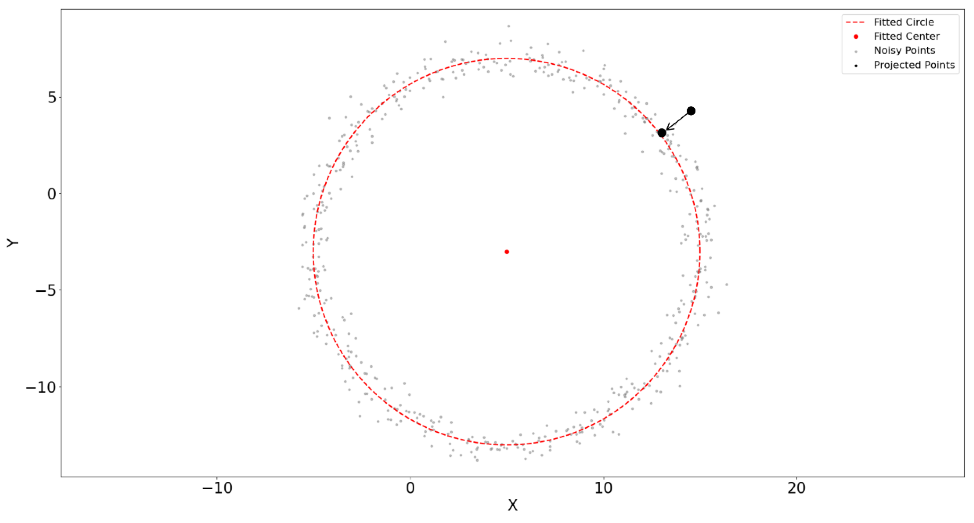
For the original point cloud, this study uses the shortest distance projection method to project each point radially onto the boundary of the fitted ellipse. The projection direction is determined by calculating the shortest path from each point to the ellipse. The principle is illustrated in Figure 9.

For each original tunnel point cloud’s XY plane coordinates $\left(x_i,y_i\right)$, the distance between the point and the center of the ellipse is calculated and normalized, as shown in Equations (18) and (19). Based on the normalized relative distance, the directional factor i for the point-cloud projection can be computed, as shown in Equation (20). Using Equations (21) and (22), the final projected point-cloud coordinates $\left({x_i}^{\prime },{y_i}^{\prime }\right)$ can be obtained, while the z-coordinate of the point cloud remains unchanged throughout the process.

$$x_{rel}=x_i-h y_{rel}=y_i-k$$

(18)

$${\widehat{x}}_{rel}={\displaystyle \frac{x_{rel}}{a}} {\widehat{y}}_{rel}={\displaystyle \frac{y_{rel}}{b}}$$

(19)

$$i=\sqrt{{{\widehat{x}}_{rel}}^2+{{\widehat{y}}_{rel}}^2}$$

(20)

$${x_i}^{\prime }=h+{\displaystyle \frac{x_{rel}}{i}} ·a$$

(21)

$${y_i}^{\prime }=k+{\displaystyle \frac{y_{rel}}{i}} ·b$$

(22)

In the equations, $x_{rel}$ and $y_{rel}$ represent the coordinate differences between each point cloud and the center of the fitted ellipse $\left(h,k\right)$. a and b denote the lengths of the semi-major axis and semi-minor axis of the fitted ellipse, respectively.

The point cloud after the coordinate system transformation and cross-section fitting denoising based on the Huber loss function can effectively remove noise points, such as pipeline and other non-structural facility point clouds, while retaining the geometric shape of the tunnel lining structure.

2.3. Evaluation Metrics Calculation

Due to the huge amount of point-cloud data, it is difficult to evaluate the denoising effect of the denoised point cloud manually. Some researchers evaluate the denoising effect of the point cloud by calculating the distribution difference of the point-cloud data before and after denoising. Bao, Yan [34] and other researchers quantitatively evaluated the denoising effect of the point cloud by calculating the maximum relative deviation (MRD), average deviation (AD), and mean square error (MSE). Wang, Z. [35] evaluated the denoising effect of the point cloud by calculating the maximum positive displacement and maximum negative displacement of the point-cloud projection before and after denoising.

To quantitatively evaluate the effectiveness of the Huber loss function-based point-cloud denoising method, this study, based on the aforementioned literature and mathematical statistical principles, employs three evaluation metrics—mean squared error (MSE), root-mean-squared error (RMSE), and mean absolute error (MAE)—to assess whether the fitted ellipse accurately matches the distribution of the original point cloud, and thereby evaluates whether the denoised point cloud retains the geometric features of the tunnel lining.

However, due to the presence of non-structural facility point clouds (such as noise points from auxiliary structures) in the original point cloud, these non-structural point clouds introduce calculation errors when evaluating the entire section. This ultimately affects the judgment of the denoising effect for the section. Therefore, directly calculating the three metrics for the entire section point cloud cannot accurately reflect the fitting and denoising performance.

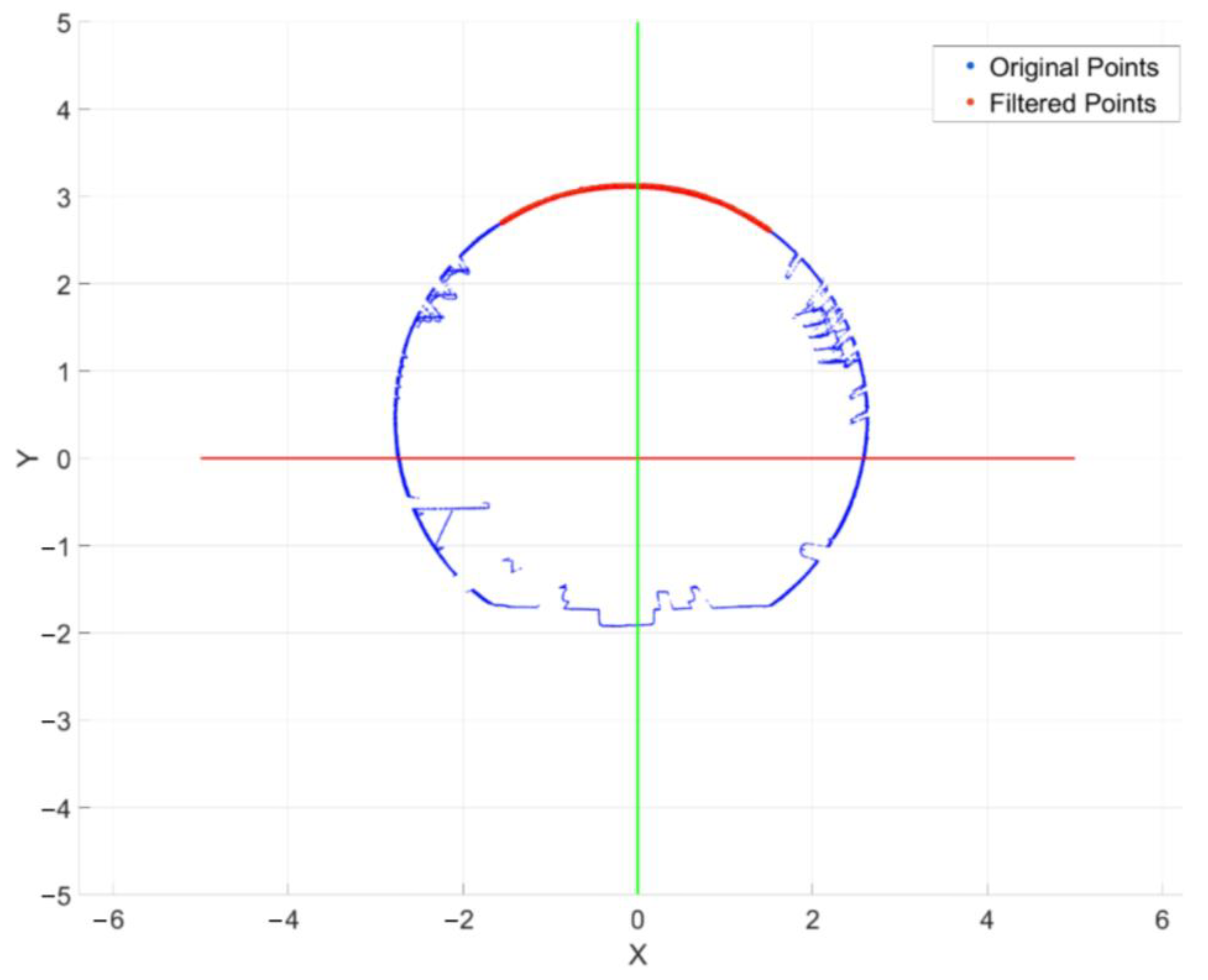
In addition to calculating the evaluation metrics for the entire section, this study also selects the local point cloud at the tunnel crown (from 60° to 120° of the tunnel cross-section, with the positive x-axis as the 0° direction) to compute the three evaluation metrics. This part of the tunnel point cloud, from the 60° to 120° range at the top of the tunnel, effectively reflects the denoising results of the tunnel lining structure since there are no non-structural facilities (noise points). As shown in Figure 10, the red area represents the selected partial point cloud.

Due to the presence of noise points (outliers), calculating the error using only the x and y coordinates in the Cartesian coordinate system for each point cloud may result in sudden value changes that affect the evaluation of the point-cloud denoising effect.

To mitigate the influence of outliers and comprehensively evaluate the denoising effect of the method in both the $x$ and $y$ coordinate directions, this study uses the distance $r_0$ from the points to the center of the fitted circle before and after projection, instead of calculating the evaluation metrics based on the $x$ and $y$ coordinates, as shown in Equation (23).

$$r_0=\sqrt{{\left(x_i-h\right)}^2+{\left(y_i-k\right)}^2}$$

(23)

This equation evaluates the difference between the fitted denoised point cloud and the tunnel-lining-structure point cloud by calculating the difference in the radius from each point to the center of the fitted circle before and after projection. Therefore, the calculation of evaluation metrics MSE, RMSE, and MAE based on the radial distances $r_0$ of the point cloud and the projected point-cloud radial distances ${r_0}^{\prime }$ is as follows:

The MSE is the average of the squared differences between the fitted values and the original values, used to quantify the overall magnitude of the error, as shown in Equation (24). The RMSE is the square root of the MSE, and it has the same units as the original data, making it more intuitive when interpreting the error magnitude. As shown in Equation (25), the lower the value of RMSE, the smaller the error.

$$\mathrm{M}\mathrm{S}\mathrm{E}={\displaystyle \frac{1}{N}}\sum _{i=1}^N{\left(r_0-{r_0}^{\prime }\right)}^2$$

(24)

$$\mathrm{R}\mathrm{M}\mathrm{S}\mathrm{E}=\sqrt{{\displaystyle \frac{1}{N}}\sum _{i=1}^N{\left(r_0-{r_0}^{\prime }\right)}^2}$$

(25)

The MAE is the average of the absolute errors of all data points, and it provides an intuitive measure of the magnitude of the error. As shown in Equation (26), the smaller the MAE, the smaller the error in the results.

$$\mathrm{M}\mathrm{A}\mathrm{E}={\displaystyle \frac{1}{N}}\sum _{i=1}^N\left|r_0-{r_0}^{\prime }\right|$$

(26)

This study calculates and evaluates the point-cloud denoising effect based on the above three metrics for both the entire cross-sectional point cloud and the tunnel-top point cloud, which contains fewer noise points.

3. Results

3.1. Data Selection

In this study, 40 m long tunnel point-cloud data from an operational subway shield-tunnel section were selected to validate the denoising effect of the proposed method. The shield-tunnel segment in this section has a width of 1.5 m, an internal radius of 2.7 m, and an external radius of 3 m.

In this study, the Amberg Clearance GRP 5000—Profiler 6012 mobile 3D laser scanning system was used for data acquisition. The system includes an Amberg Profiler 6012 high-speed phase laser scanner, a Distance Measurement Instrument (DMI), a high-precision inertial navigation unit, an industrial-grade laptop computer, and a composite frame accessory, as shown in Figure 11.

The distance measurement principle of this model of scanner is phase-based interferometric ranging, which determines distances by analyzing the phase shift of reflected laser signals. The scanner operates at a maximum frequency of 200 Hz, with a scanning range covering a 360° horizontal field of view and a vertical field of view of 120° or greater. It supports a maximum measuring distance of 119 m and a maximum sampling rate of 1.016 million points per second. The ideal measurement accuracy is 0.1 mm. In actual scanning operations, the device moves forward at a speed of 4 km/h and collects 5000 points per profile. The device can operate stably in environments ranging from −10 °C to 50 °C, generating tens of thousands to millions of point-cloud data per second. The device supports multiple file output formats such as LAS and ASCII. The point-cloud data from actual tunnel scans are shown in Figure 12.

In this study, to ensure that each cross-section has enough point clouds for ellipse-fitting while maintaining an appropriate cross-sectional thickness, one cross-section is extracted every 0.1 m along the z-axis for the transformed point cloud (where the tunnel axis direction is parallel to the z-axis). For each extracted cross-section, the Huber loss function is used for ellipse-fitting, and the original point cloud is projected based on the minimum radial distance to achieve denoising. The denoising effects for individual cross-sectional point clouds and the entire-tunnel point cloud are shown in Section 3.2 and Section 3.3.

3.2. Denoising Effect of Individual Cross-Sectional Point Clouds

To evaluate the denoising effect of individual cross-sections, five cross-sections were randomly extracted from the tunnel point-cloud data for assessment. At the same time, for the convenience of management and experimental needs, this study named these five cross-sections Sections 1–5, as shown in Figure 13. Each section in the figure is a tunnel point-cloud dataset with a thickness of 0.1 m. In order to ensure the rigor of the experiment, the distance between sections in the figure is a random value. The number of point clouds contained in each cross section is shown in

Table 1. Statistics of point-cloud quantity for individual cross-sections.

Section Number	Section 1	Section 2	Section 3	Section 4	Section 5
Point-cloud quantity	65,583	75,196	67,447	66,256	67,689

.

To visualize the denoising effect of individual cross-section point clouds, Section 1 is taken as an example. The ellipse-fitting and point-cloud denoising effects are shown in Figure 14, where the blue points represent the original point cloud and the red points represent the denoised point cloud after fitting.

To quantitatively assess the effectiveness of the point-cloud denoising method in this study, three evaluation metrics—MSE, RMSE, and MAE—are introduced. These metrics reflect the similarity between the denoised point cloud and the entire-tunnel cross-section’s lining structure. The evaluation results for the entire cross-section are shown in

Table 2. Evaluation metrics calculation results for an individual tunnel cross-section.

Evaluation Metrics	Section 1	Section 2	Section 3	Section 4	Section 5	Average Value
$\mathrm{M}\mathrm{S}\mathrm{E}\left({\mathrm{m}}^2\right)$	0.05069	0.05336	0.04493	0.05318	0.08357	0.05715
$\mathrm{R}\mathrm{M}\mathrm{S}\mathrm{E}\left(\mathrm{m}\right)$	0.22515	0.23101	0.21197	0.23060	0.28909	0.23756
$\mathrm{M}\mathrm{A}\mathrm{E}\left(\mathrm{m}\right)$	0.13563	0.13612	0.12251	0.13517	0.18281	0.14245

.

$\mathrm{M}\mathrm{S}\mathrm{E}\left({\mathrm{m}}^2\right)$$\mathrm{R}\mathrm{M}\mathrm{S}\mathrm{E}\left(\mathrm{m}\right)$$\mathrm{M}\mathrm{A}\mathrm{E}\left(\mathrm{m}\right)$ The analysis of the evaluation metric results for the entire cross-section indicates that the point cloud processed by the Huber loss-based ellipse-fitting denoising method is in general agreement with the original tunnel point-cloud lining structure. However, due to the presence of noise points, these evaluation metrics do not accurately reflect the fitting denoising effect on the tunnel lining structure without noise points. Therefore, this study also separately selects the tunnel-top (60°–120°) point cloud for evaluation metric calculation, and the results are shown in

Table 3. Evaluation metric calculation results for the tunnel-top (60°–120°) point cloud of an individual tunnel section.

Evaluation Metrics	Section 1	Section 2	Section 3	Section 4	Section 5	Average Value
$\mathrm{M}\mathrm{S}\mathrm{E}\left({\mathrm{m}}^2\right)$	0.00006	0.00022	0.00004	0.00013	0.00029	0.00015
$\mathrm{R}\mathrm{M}\mathrm{S}\mathrm{E}\left(\mathrm{m}\right)$	0.00806	0.01504	0.00667	0.01149	0.01690	0.01163
$\mathrm{M}\mathrm{A}\mathrm{E}\left(\mathrm{m}\right)$	0.00642	0.01185	0.00477	0.00878	0.01444	0.00925

.

From the evaluation metrics in Table 3, it can be seen that the geometric parameters of the tunnel cross-sectional top point cloud, after denoising using the Huber loss-based point-cloud denoising method, are highly consistent with those of the actual tunnel lining structure’s top point cloud, with errors reduced to the millimeter level.

At the same time, the evaluation results in Table 3 are significantly lower than those in Table 2. This is because, in the evaluation metrics calculated for Table 2, the original point cloud used as the benchmark contains noise points such as tunnel pipelines, and these noise points introduce errors in the evaluation metrics, erroneously reflecting the congruence between the denoised point cloud and the actual tunnel lining structure’s point cloud, thus leading to inflated values. In contrast, the tunnel-top point cloud contains fewer noise points, so the evaluation metrics computed for this portion more accurately reflect the denoising effect on the tunnel lining structure.

From the above results, it can be concluded that the ellipse-fitting denoising method based on the Huber loss function achieves good fitting and denoising results for the lining structure point cloud of a single tunnel section.

3.3. Denoising Effect of the Entire-Tunnel-Section Point Cloud

The denoising results of the selected 40 m long tunnel point-cloud data using the Huber loss function-based ellipse-fitting method are shown in Figure 15.

For the entire-tunnel point cloud, to quantitatively evaluate the denoising effect of the point cloud, the denoising evaluation metrics for all sections of the tunnel are calculated and shown in

Table 4. Statistical table of denoising evaluation metrics for the entire-tunnel point cloud.

Evaluation Metrics	$\mathbf{M}\mathbf{S}\mathbf{E}\left({\mathbf{m}}^2\right)$	$\mathbf{R}\mathbf{M}\mathbf{S}\mathbf{E}\left(\mathbf{m}\right)$	$\mathbf{M}\mathbf{A}\mathbf{E}\left(\mathbf{m}\right)$
Result	0.04337	0.20412	0.12645

. Additionally, for all sections of the tunnel, this study selects the local point cloud at the tunnel top (60°–120°) to compute the evaluation metrics, as shown in

Table 5. Statistical table of denoising evaluation metrics for the tunnel-top point cloud (60°–120°).

Evaluation Metrics	$\mathbf{M}\mathbf{S}\mathbf{E}\left({\mathbf{m}}^2\right)$	$\mathbf{R}\mathbf{M}\mathbf{S}\mathbf{E}\left(\mathbf{m}\right)$	$\mathbf{M}\mathbf{A}\mathbf{E}\left(\mathbf{m}\right)$
Result	0.00034	0.01447	0.01118

.

According to the evaluation metrics in Table 4 and Table 5, the denoising performance of the Huber loss-based point-cloud denoising method applied to the entire-tunnel point cloud shows no significant difference compared to that on a single tunnel cross-section point cloud. This indicates that the method exhibits a certain degree of robustness and can effectively denoise point clouds from various tunnel cross-sections.

Similar to the case in Table 2 and Table 3, the results in Table 5 show a significant improvement over those in Table 4, further demonstrating that the original point cloud—containing noise such as tunnel pipelines—introduces errors in the evaluation metrics that misrepresent the denoising performance. In contrast, the evaluation metrics computed for the tunnel-top point cloud directly assess the denoising effect on the tunnel-lining-structure point cloud, thereby providing a more accurate reflection of the denoising performance on the tunnel lining structure.

In summary, the ellipse-fitting denoising method based on the Huber loss function demonstrates good denoising performance for the entire-tunnel point cloud. It effectively preserves the geometric features of the tunnel lining structure and removes non-structural facilities, such as pipelines, from the point cloud.

4. Discussion

From the experimental results that we have reported in the previous section, it can be seen that the point-cloud denoising method based on the Huber loss function can effectively denoise the point-cloud data of the shield-tunnel section, and the highest accuracy can reach the millimeter level. This method demonstrates good denoising performance for both individual cross-sectional point clouds and the entire-tunnel point cloud, indicating its robustness to complex noise distributions.

This robustness is due to the fact that the Huber loss function uses squared error for small deviations—making it highly sensitive to minor errors—and linear error for large deviations, thereby reducing the influence of outliers or anomalous points on the overall fitting result. This characteristic ensures that noise from non-structural facilities such as pipelines does not excessively interfere with the final fitting, thus allowing for the accurate extraction and denoising of the main tunnel structure (tunnel lining structure).

Moreover, the Huber loss function exhibits smoother error variations, combining the high precision of mean squared error when the data are relatively clean with the robustness of absolute error when handling noisy data, thereby enabling effective denoising even for tunnel-top point clouds that contain fewer noise points.

In order to evaluate the merits and drawbacks of the denoising performance of the proposed method, this study compares the denoising effect of the elliptical-fitting denoising method based on the Huber loss function with that of a widely used free point-cloud processing software. Taking into account factors such as the user base and whether the software is open source, this study selected CloudCompare version 2.10 as the benchmark for the denoising performance comparison.

CloudCompare is an open-source 3D point-cloud processing software that focuses on handling high-density point-cloud data and 3D meshes. Its primary functions include point-cloud alignment, registration, segmentation, denoising, resampling, and geometric feature extraction, among others. This software is widely used in point-cloud data processing tasks in fields such as engineering surveying and archaeological mapping.

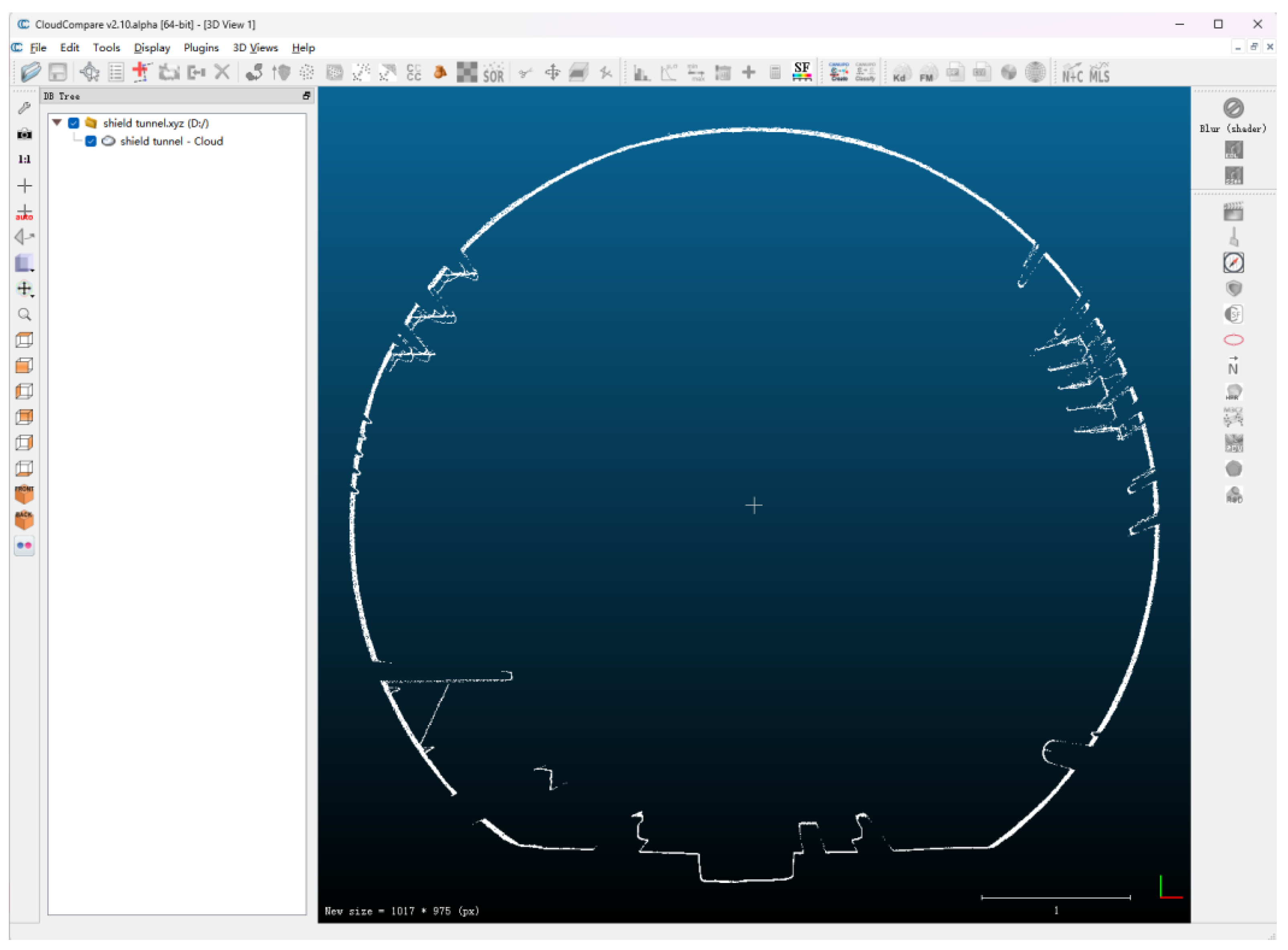
In this study, tunnel point-cloud data were denoised using CloudCompare software version 2.10, with the software interface shown in Figure 16. CloudCompare allows for denoising by manually selecting and removing points from the cloud. However, due to the enormous volume of tunnel point-cloud data, manually denoising the data consumes a considerable amount of time and manpower. Moreover, manual denoising often introduces human errors, which can affect the accuracy of the denoising process.

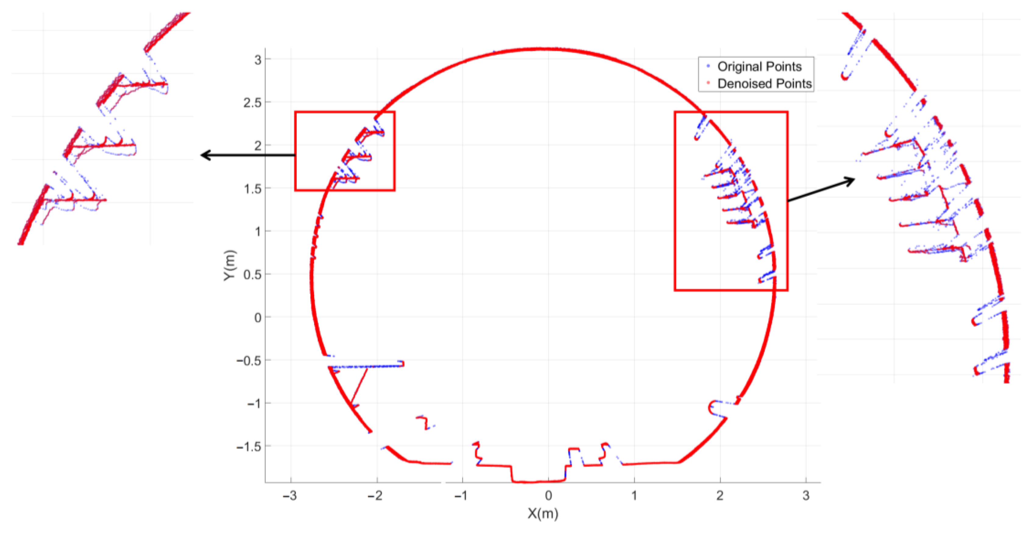
In addition, CloudCompare software also includes a statistical outlier removal (SOR) filtering denoising function that can automatically denoise point clouds. The denoising effect is shown in Figure 17, where blue represents the original point cloud and red represents the denoised point cloud. As can be seen from the results, point-cloud denoising based on the SOR filter in CloudCompare is capable of removing some outlier points from tunnel point clouds; however, it is difficult to remove noise with a continuous spatial distribution, such as pipeline point clouds.

To further discuss the effectiveness of the ellipse-fitting and point-cloud denoising method proposed in this study, we compare it with two widely used fitting and denoising methods: the least-squares method and random sample consensus (RANSAC) method.

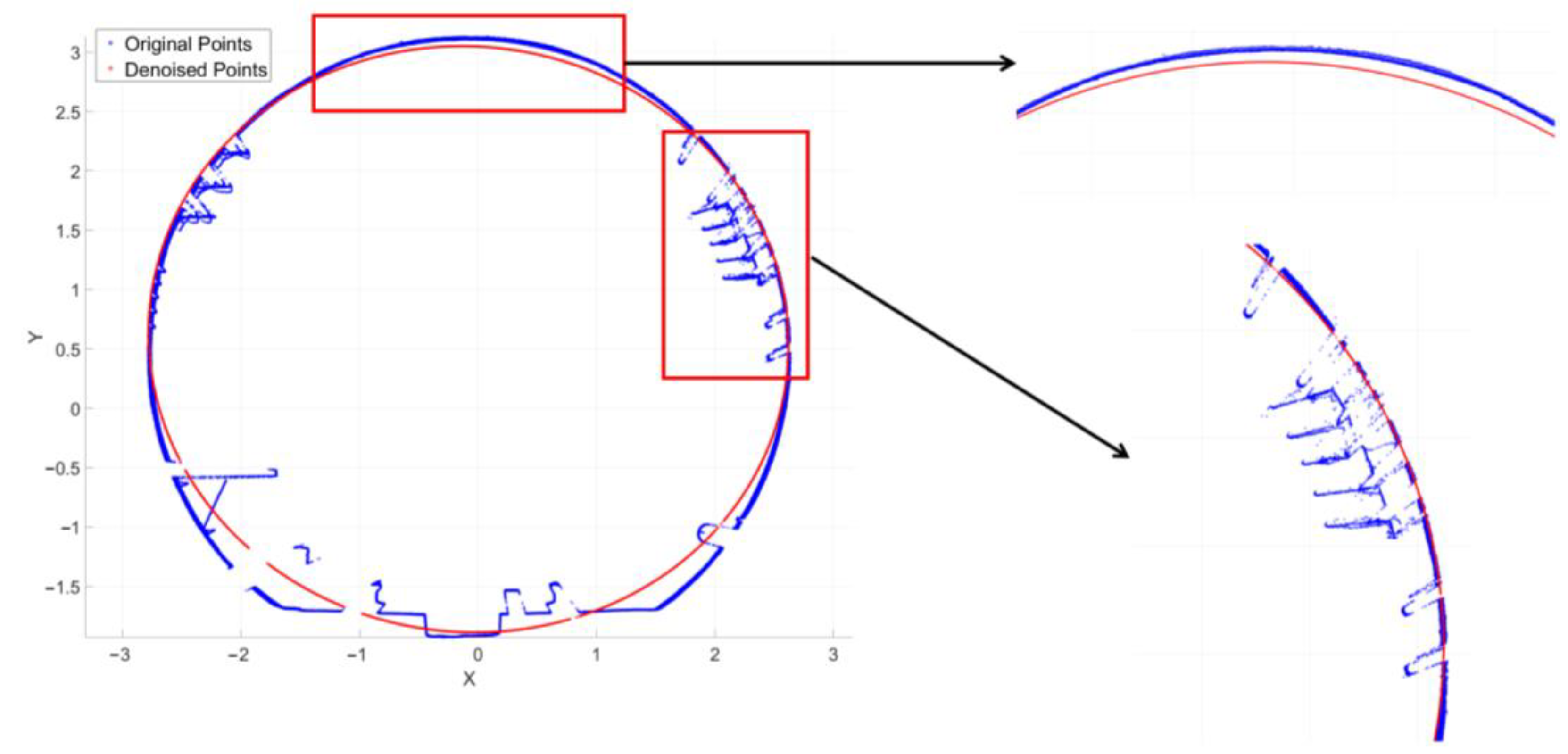
The least-squares method is a fitting approach based on the sum of squared errors. It minimizes the squared differences between the actual data values and the fitted function to obtain the optimal fitting ellipse. By projecting the point cloud onto the fitted ellipse, denoising is achieved. This method is widely used in various data fitting tasks due to its simple algorithmic structure and other advantages. As described in the previous section, this study extracted five sections from a 40 m long tunnel for denoising. In order to more intuitively and scientifically compare the denoising effects of the least-squares method and the method proposed in this study, this study performed denoising on the same section (Section 1 in 3. Results). The denoising result is shown in Figure 18, where the blue points represent the original point cloud and the red points represent the denoised point cloud after fitting.

Random sample consensus (RANSAC) is an iterative fitting method based on random sampling. It randomly selects a subset of data, treating points that are close to the fitted ellipse as inliers and points that are far from the fitted ellipse as outliers (noise points). Through iterative sampling and estimation of model parameters, RANSAC ultimately obtains the optimal fitted ellipse. This method is widely used in fitting and denoising tasks due to its robustness to noise, ability to handle various fitting models, and other advantages.

In order to compare the denoising effect of the method proposed in this study, the RANSAC method is used to denoise Section 1 extracted in the previous stages (or steps) of the work. The denoising results are shown in Figure 19, where the blue points represent the original point cloud and the red points represent the denoised point cloud after fitting.

As shown in the above figures, both the least-squares method and RANSAC method can perform fitting and denoising on a single subway tunnel section. To quantitatively assess the denoising effectiveness of these two methods in comparison with the method proposed in this study, the evaluation metrics are calculated for the point cloud of all cross-sections of the entire tunnel as well as the selected top tunnel point cloud (60°–120°) of each section. The average values of the evaluation metrics for all cross-sections are calculated, and the results are compared with those of the Huber loss-based method proposed in this study. The calculation results are shown in

Table 6. Statistical table of evaluation metrics for denoising of the whole tunnel section point cloud.

Fitting Denoising Method	$\mathbf{M}\mathbf{S}\mathbf{E}\left({\mathbf{m}}^2\right)$	$\mathbf{R}\mathbf{M}\mathbf{S}\mathbf{E}\left(\mathbf{m}\right)$	$\mathbf{M}\mathbf{A}\mathbf{E}\left(\mathbf{m}\right)$
Huber loss-based method	0.04920	0.21655	0.13257
Least-squares method	0.01958	0.13964	0.10187
RANSAC method	0.01961	0.13969	0.10066

and

Table 7. Statistical Table of denoising evaluation metrics for tunnel section top point cloud (60°–120°).

Fitting Denoising Method	$\mathbf{M}\mathbf{S}\mathbf{E}\left({\mathbf{m}}^2\right)$	$\mathbf{R}\mathbf{M}\mathbf{S}\mathbf{E}\left(\mathbf{m}\right)$	$\mathbf{M}\mathbf{A}\mathbf{E}\left(\mathbf{m}\right)$
Huber loss-based method	0.00033	0.01383	0.01061
Least-squares method	0.00184	0.04157	0.03857
RANSAC method	0.00269	0.05098	0.04850

.

In addition, this study also recorded the time required for these three methods to process the same data (the entire 40 m long tunnel point cloud) under the same experimental conditions, including computer performance and system environment. The results are shown in

Table 8. Comparison of algorithm running time.

Fitting Denoising Method	Huber Loss-Based Method	Least-Squares Method	RANSAC Method
Algorithm Running Time	1 min 33 s	20 s	11 h 48 min 43 s

.

Based on the actual fitting effect images and the calculated evaluation metrics, it can be observed that both the least-squares method and RANSAC can fit ellipses that approximately match the tunnel section. However, these two methods are significantly affected by noise, resulting in fitting outcomes that deviate considerably from the actual geometric characteristics of the tunnel lining structure.

Additionally, due to the iterative nature of the RANSAC method in searching for the optimal model, its computational efficiency is relatively lower. Furthermore, both the least-squares method and RANSAC exhibit poor fitting results for the lower part of the tunnel lining structure. In contrast, the ellipse-fitting method based on the Huber loss function can effectively perform fitting and denoising for tunnel point clouds containing noise. The fitting results align closely with the tunnel lining structure, and the method maintains good computational efficiency.

5. Conclusions

LiDAR is widely used in tunnel and other construction structure measurement and inspection due to its advantages such as non-contact measurement, fast data acquisition speed, and high automation. However, the presence of non-structural facilities, such as pipelines, within tunnel structures can interfere with the detection of tunnel lining structures. To address the noise point clouds, this study proposes a tunnel cross-section fitting and projection denoising method based on the Huber loss function, as well as a point-cloud coordinate system transformation method. The research has achieved the following outcomes:

1. A tunnel cross-section point-cloud ellipse-fitting and denoising method based on the Huber loss function and the shortest radial distance projection is proposed. This method can denoise raw tunnel point-cloud data without preprocessing, effectively removing noise points while preserving the geometric features of the tunnel lining, and it has good computational efficiency.

2. A method based on PCA and Huber loss function for tunnel point-cloud coordinate transformation was proposed. This method effectively transforms the tunnel point-cloud coordinate system, aligning the tunnel point-cloud data with the Cartesian coordinate system axes (orthogonally), reducing the errors caused by manually rotating the point cloud during the denoising process.

3. When evaluating the denoising effect, in addition to calculating the entire point-cloud section, the top point cloud with fewer non-structural facility point clouds on the top of the tunnel was also selected for calculation, which more comprehensively reflects the denoising effect of the tunnel point cloud.

In the next phase of this work, we will continue to improve the algorithm and optimize the denoising effect of the method on the bottom point cloud (tunnel-track point cloud). At the same time, the method will be adjusted to effectively denoise point-cloud data for more complex tunnel structures, such as non-circular tunnels and curved tunnels.