Physics-Guided Neural Network-Based Feedforward Control for Seamless Pipe Manufacturing Process

Abstract

Artificial intelligence (AI) is increasingly being utilized in the industrial sector, revolutionizing traditional manufacturing processes with advanced automation systems. Despite their potential, neural networks have seen limited adoption in industrial control systems due to their lack of interpretability compared to traditional methods. The recently introduced physics-guided neural networks (PGNNs) address this limitation by embedding physical knowledge directly into the network structure, enhancing the interpretability and robustness. This study proposes a novel feedforward control framework that integrates a reduced-order physics-based model of a hydraulic actuator with a data-driven correction term for accurate force control in the seamless pipe manufacturing process. The coupled dynamics of the actuator and the continuously cast material being pushed into the piercing mill are identified through experimental data, and reduced-order models are developed for integration into the PGNN structure. The training of the networks is performed on a dataset from a scaled industrial hydraulic system, with the validation of the proposed methods conducted on a neural processing unit (NPU), a specialized industrial-grade platform for AI, operating within a PLC environment. The results demonstrate real-time execution with excellent force tracking, even with a limited training dataset—a typical constraint in industrial processes—while providing safer and more predictable behavior compared to traditional neural-network-only solutions.

1. Introduction

Steel pipes are produced using several manufacturing processes, with the most common ones being seamless pipe manufacturing and welded pipe manufacturing. Seamless pipe manufacturing involves heating a solid steel billet, which is then pierced to create a hollow tube. The Mannesmann process uses a rotary piercing machine to create a hollow tube, with two rollers rotating in the same direction and set at an angle to the pipe’s centerline, followed by rolling and stretching to achieve the final dimensions [1].

Seamless pipes are often used where strength and resistance to pressure are critical, such as in the oil and gas industry. Among several factors that dictate the quality of the final product during the Mannesmann process, the piercing process is central to achieving optimal results. Precise control of the piercing force is essential because any deviations can lead to defects, such as uneven wall thicknesses, off-center holes, and surface irregularities, compromising the integrity of the final pipe.

In modern variations of this process, a continuously cast material is often used instead of traditional billets, offering improved efficiency by eliminating the intermediate steps of casting and reheating [2].

To ensure smooth and precise operation during the piercing process, an entrance device is employed to continuously guide the cast material into the piercing mill. This device commonly consists of hydraulic actuators that provide the desired pushing force needed to maintain consistent material feeding. The accurate control of this force is important in preventing issues that can negatively impact the quality of the final product.

Feedforward control is a widely used technique in control system design, particularly effective in addressing predictable disturbances and ensuring precise trajectory tracking. By leveraging a model of the system or process, feedforward controllers generate control actions based on reference inputs, proactively mitigating deviations before they occur [3,4]. This approach complements feedback control, which reacts to errors after they are detected, reducing the burden on feedback loops and enabling faster system responses—especially in dynamic and complex industrial environments [5].

Traditional feedforward control techniques often rely on mathematical models derived from system dynamics or empirical data obtained through experiments [6,7]. However, classical methods face challenges in handling model uncertainties, nonlinearities, and unforeseen disturbances [8].

In response to these challenges, neural networks (NNs) have emerged as a powerful tool for the design of feedforward controllers due to their universal approximation capabilities [9]. Neural networks can learn complex, nonlinear relationships directly from experimental data, bypassing the need for highly accurate mathematical models. Sørensen [10] demonstrated the efficacy of NN-based feedforward control in managing nonlinear system dynamics, while Li et al. [11] applied adaptive NN feedforward strategies to dynamically substructured systems. Despite their flexibility and ability to model complex behaviors, NN-based approaches often require large datasets spanning the full operating range to ensure reliable performance [12,13].

To address the limitations of standard NN approaches, physics-informed neural networks (PINNs) have been introduced. PINNs embed physical laws, often expressed as partial differential equations (PDEs), directly into the network’s training process [14]. This integration reduces the dependence on extensive datasets and enhances the generalization of the model across varying operating conditions. Bolderman et al. [15] demonstrated the application of PINNs in feedforward control, showing improved robustness and interpretability under diverse scenarios.

Building upon the foundation of PINNs, physics-guided neural networks (PGNNs) represent a significant step forward in control system design. PGNNs not only incorporate physical insights into the training process but also embed structured physical models directly into the neural network architecture [16]. This structured approach enhances the interpretability, ensures compliance with system dynamics, and improves the robustness against varying operating conditions. This fusion allows for a reduced dependence on large datasets, especially in scenarios where data availability is limited or where the system operates outside the conditions used for training.

In the context of feedforward control, PGNNs have demonstrated their effectiveness in predicting and compensating for system disturbances and nonlinearities. Fan et al. [17] successfully applied PGNNs as feedforward controllers in hybrid stepper motors, and Kon et al. [18] applied PGNNs as feedforward controllers in precision motion control systems, both demonstrating improved tracking accuracy and performance. Bolderman et al. [19] demonstrated the effectiveness of PGNNs in addressing nonlinearities and parasitic effects within industrial systems, specifically when applied in feedforward control architectures requiring precise compensation and preemptive adjustments.

Previous studies on PGNNs have predominantly focused on electromechanical actuator systems, where feedforward controllers are primarily used to compensate for friction. These systems benefit from the relatively isolated nature of their dynamics, allowing the PGNN to focus on accurately modeling the actuator’s behavior. Although this approach has proven to be effective, it overlooks the critical influence of coupled dynamics in systems where the actuator interacts directly with the processed material in the production processes in heavy industry.

In hydraulic actuators, this coupling becomes particularly significant due to the inherent relationship between the movement of the actuator’s rods, the resulting pressure changes, and the corresponding actuation forces. Unlike electromechanical systems, where the force generation mechanism is more straightforward, hydraulic systems must contend with dynamic interactions between the actuator and the load. These interactions are further complicated in industrial applications where the production process itself introduces additional resistive forces and disturbances that must be accounted for in the control strategy.

To address this, our work extends the application of PGNNs to hydraulic actuators, marking, to the best of our knowledge, the first attempt to incorporate this methodology in such systems. We innovatively couple the dynamics of the hydraulic actuator with the dynamics of the production process within the physical part of the PGNN. By doing so, we create a more comprehensive and robust feedforward structure that is able to capture the interactions between the actuator and the production process.

We also address the significant challenge in industrial applications, which has traditionally been the lack of hardware platforms capable of executing such neural networks in real time within the control loop.

In earlier implementations, such as those described by Ahmad and Prajitno [20], neural networks were executed on external computers, with communication to PLCs managed via OPC protocols. This setup inherently limited the system’s ability to perform in real-time scenarios due to latency issues and the absence of hard real-time communication capabilities.

The introduction of specialized hardware, such as Siemens’ neural processing unit (NPU), represents a transformative step towards the seamless integration of AI into industrial automation systems. These processors, originally designed for applications like image recognition and classification [21,22], have now been adapted for the execution of neural network-based control algorithms directly within the PLC environment. Compared to external GPU-based setups, like those described by Schmidt et al. [23], where reinforcement learning methods were applied using GPU-accelerated industrial control hardware, the Siemens NPU offers a streamlined, cost-effective solution with lower power consumption and easier integration into existing PLC systems. Its ability to execute neural network algorithms directly within PLCs ensures minimal latency, enhanced responsiveness, and consistent high-quality performance.

This paper is organized as follows. First, mathematical models of the hydraulic actuator and the combined dynamics of the actuator and external resistive forces are developed, and unknown parameters are identified. These models are then reduced to a form suitable for integration into the PGNN framework. The theoretical background of PGNNs tailored to specific application is presented, followed by a description of the experimental setup, which consists of a scaled industrial hydraulic system used for both training and validation.

Next, the training results of the PGNN are presented alongside a benchmark neural network used for comparison. Finally, the proposed methods are validated through two sets of experiments: one focusing on constant force setpoint tracking with varying speeds and another on varying force tracking with speed profiles representative of the operational conditions in pipe manufacturing. Conclusions are then drawn to summarize the findings and highlight future directions.

2. Materials and Methods

2.1. Mathematical Models

Since knowledge of the system characteristics is desirable for the purpose of controller synthesis, this section will present the mathematical models of the hydraulic actuator and the external resistance force. Modeling the external force is essential in testing the proposed control algorithm on simulation hardware in the absence of a real pipe production system.

2.1.1. Hydraulic Actuator

In the following text, the mass of the moving parts is denoted with m (the mass of the piston and the accompanying parts moved by the piston), the piston’s velocity with v, and the piston’s position (measured from the midpoint of the actuator’s stroke) with x.

The equations describing the movement of the piston are as follows:

$$m{\displaystyle \frac{dv}{dt}}=F_{act}-F_{int}-F_{ext},$$

(1)

$${\displaystyle \frac{dx}{dt}}=v.$$

(2)

The actuation force $F_{act}$ is obtained on the basis of the pressure difference in the cylinder chambers:

$$F_{act}=p_A{A}_A-p_B{A}_B,$$

(3)

where $A_A$ and $A_B$ are the piston-side area and rod-side area, respectively.

The equations that describe the pressure change in the cylinder chambers are

$${\displaystyle \frac{V_A}{\beta }}{\displaystyle \frac{d{p}_A}{dt}}+A_{A}v=Q_A-C_i\left(p_A-p_B\right),$$

(4)

$${\displaystyle \frac{V_B}{\beta }}{\displaystyle \frac{d{p}_B}{dt}}-A_{B}v=-Q_B+C_i\left(p_A-p_B\right)-C_e{p}_B,$$

(5)

where $\beta$ is the bulk modulus of the hydraulic oil. The volumes of the chambers depend on the position of the piston:

$$V_A=V_{A0}+A_{A}x,$$

(6)

$$V_B=V_{B0}-A_{B}x.$$

(7)

The coefficients $C_i$ and $C_e$ account for fluid leaks between the chambers and the external environment. Many hydraulic actuators are designed with high-quality seals, which reduce the external leakage to a level that does not significantly affect the performance, making it negligible unless the system operates under conditions where seal degradation is a concern. Internal leakage primarily accounts for the pressure drop due to minor fluid penetration between the actuator chambers, influenced by factors such as cylinder wear—related to the hydraulic cylinder’s life cycle—temperature-dependent expansion, and the fluid viscosity.

To obtain a reduced-order model that is suitable for real-time integration with data-driven methods due to its simplicity, external leakage is neglected in this study as this simplifies the model without compromising the accuracy. Internal leakage will be considered in the identification process of the fully nonlinear actuator model but is also neglected in the reduced-order modeling since its contribution to the actuator behavior is minor in well-maintained systems with intact seals. This approach is standard in many hydraulic actuator modeling methods (e.g., [24,25]), particularly in linearized models used for control system synthesis.

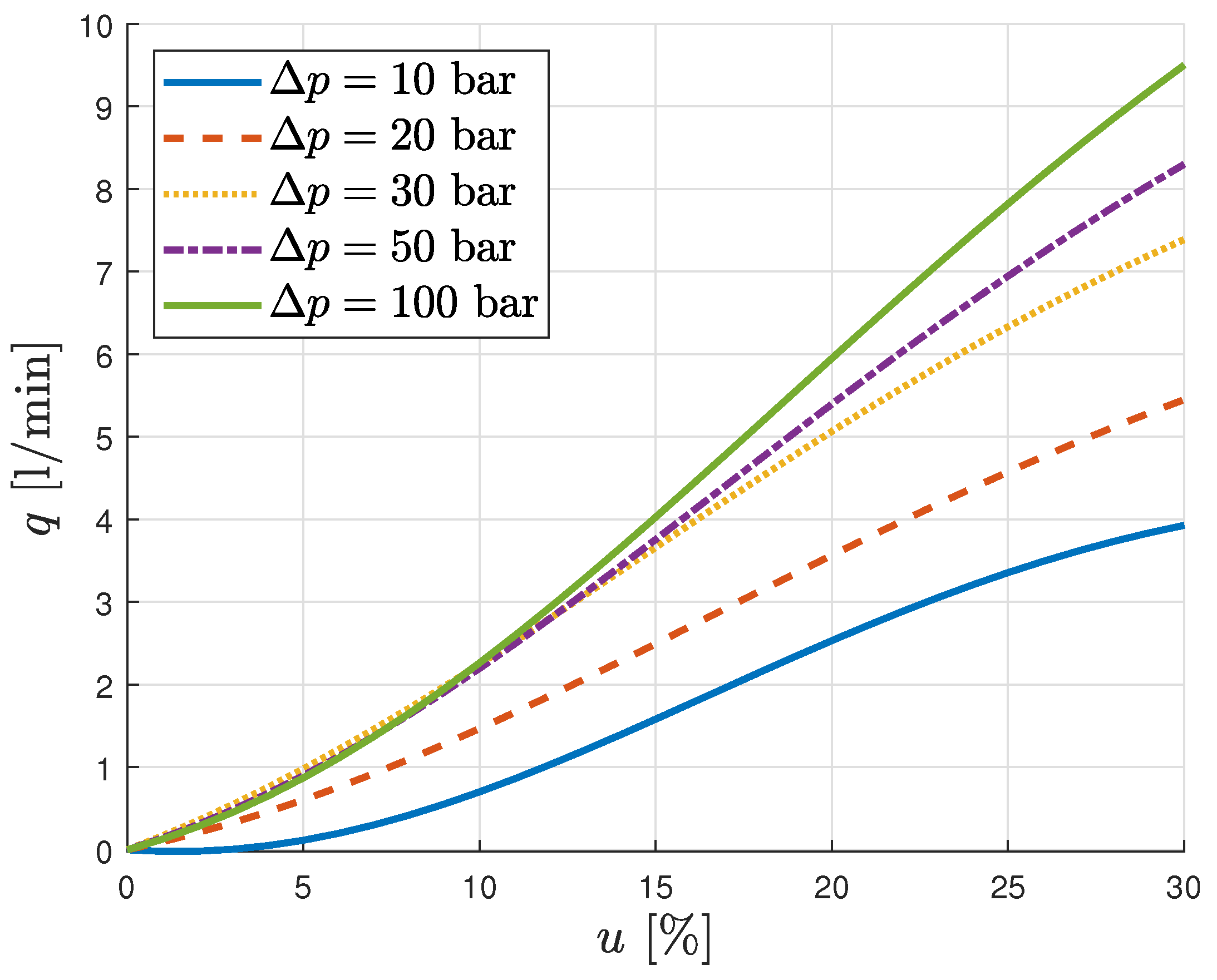
The flows $Q_A$ and $Q_B$ are determined based on the opening of the directional valve (u) and the pressure difference at the inlet and outlet of the valve ($\Delta p$):

$$Q=Q\left(u,\Delta p\right).$$

(8)

This relationship is described by the manufacturer’s specifications and is illustrated in Figure 1.

The primary task of the controller is to determine the valve opening u in order to ensure a constant material pressing force $F_{act}$.

The term $F_{int}$ in Equation (1) models the internal resistances to the movement of the piston that occur within the cylinder itself. In general, this term represents a function of the piston’s velocity and position and may depend on how the cylinder is oriented (e.g., if the cylinder is positioned vertically, this term also includes the gravitational force acting on the piston). The equation modeling the internal resistances to the piston’s movement takes the form of the Stribeck friction curve [24]:

$$F_{int}=F_{int0}+\sigma v+\mathrm{sgn}\left(v\right)\left[F_{c0}+F_{s0}\exp \left(-{\displaystyle \frac{\left|v\right|}{c_s}}\right)\right],$$

(9)

where $\sigma$ is the parameter for viscous friction, $F_{c0}$ is the parameter for Coulomb friction, and $F_{s0}$ and $c_s$ are the parameters for static friction. The first component in Equation (9) models a constant load, which is independent of the direction of the piston’s velocity. This resistance component does not exist, as this work considers horizontally positioned cylinders.

Parameters $\sigma$, $F_{c0}$, $F_{s0}$, $c_s$ from Equation (9) and parameters $C_i$, $C_e$ from Equations (4) and (5) are unknown and need to be determined. One method of determining these parameters is to use least squares fitting based on experimentally recorded data [26]. For this study, the system response was recorded as the piston speed for step valve opening inputs with different amplitudes. The experiment was conducted with a free cylinder, i.e., without the presence of additional external forces ($F_{ext}=0$).

A comparison between the experimentally recorded responses and data from the simulation model is shown in Figure 2. The values of the parameters used in the simulation model are shown in

Table 1. Simulation model parameter values.

Parameter	Value
m	10 [kg]
$A_A$	1257 [mm2]
$A_B$	616 [mm2]
$\beta$	1.5 × 109 [Pa]
$p_S$	55 [bar]
$p_T$	1 [bar]
$V_{A0}$	2.136283 × 10−4 [m3]
$V_{B0}$	1.089504 × 10−4 [m3]

and

Table 2. Values of leakage coefficients and internal resistance force parameters.

Parameter	Value
$C_i$	0.006 [L/bar]
$C_e$	0 [L/bar]
$\sigma$	2000 [N s/m]
$F_{c0}$	400 [N]
$F_{s0}$	300 [N]
$c_s$	0.001 [m/s]

.

2.1.2. External Force

The rotary piercing process is the first forming operation in the conversion of a solid circular billet into a seamless tube [1]. Two barrel-shaped rolls (Figure 3) rotating in the same direction, whose axes are at an angle to the workpiece, provide the longitudinal component of the force and pull the billet forward. For this process to occur, an entrance device is required to guide the workpiece into the piercing mill.

When the billet meets the piercing point, the grip of the rolls is sufficient to continue the advancement of the workpiece against the retarding effect imposed by the piercing point [1]. The smooth operation of the piercing process can be completed if the following condition is satisfied [27]:

$$2T_x\ge 2P_x+Q^{\prime },$$

(10)

which relates the axial components of the friction of roll (T), the positive pressure of roll (P), and the resistance of the plug nose ($Q^{\prime }$).

The internal dynamics of the process within the mill have been extensively studied in the existing force and stress analysis literature (Refs. [1,27,28,29,30]). In this work, a simplified model to capture the dynamics outside the piercing mill is proposed. This model is primarily based on two key factors that dominate inside the mill, namely friction and material characteristics described by the stress–strain relationship, from which it is known that the resistive force of the material will initially increase in response to the pushing force until it reaches its yield stress and begins to deform. When the material starts to move, a further increase in the pushing force will cause the material to progress through the entrance of the mill, which will increase the friction force, eventually leading to a steady-state velocity corresponding to the current applied pushing force. Therefore, the following model for the resistive force as observed from the controller’s perspective outside the mill is proposed:

$$F_{ext}=\left\{\begin{array}{cc}{F}_p,\hfill & F_p<F_{yield}\hfill \\ F_{yield}+\mathcal{F}(\Delta F),\hfill & F_p\ge F_{yield}\hfill \end{array}\right.,$$

(11)

$$\Delta F=F_p-F_{yield},$$

(12)

where $F_p=F_{act}-F_{int}$ is the applied pushing force, and $F_{yield}$ is the pushing force threshold after which the material starts to deform.

Function $\mathcal{F}$ represents the resistive force delay, through which the lag between the increase in pushing force and the corresponding rise in friction (which occurs as the workpiece velocity gradually increases) is modeled. This delay will be presented with the transfer function

$${\displaystyle \frac{\mathcal{F}\left(s\right)}{\Delta F\left(s\right)}}={\displaystyle \frac{1}{{\tau }_{ext}s+1}},$$

(13)

where time constant ${\tau }_{ext}$ can be determined based on experimental data.

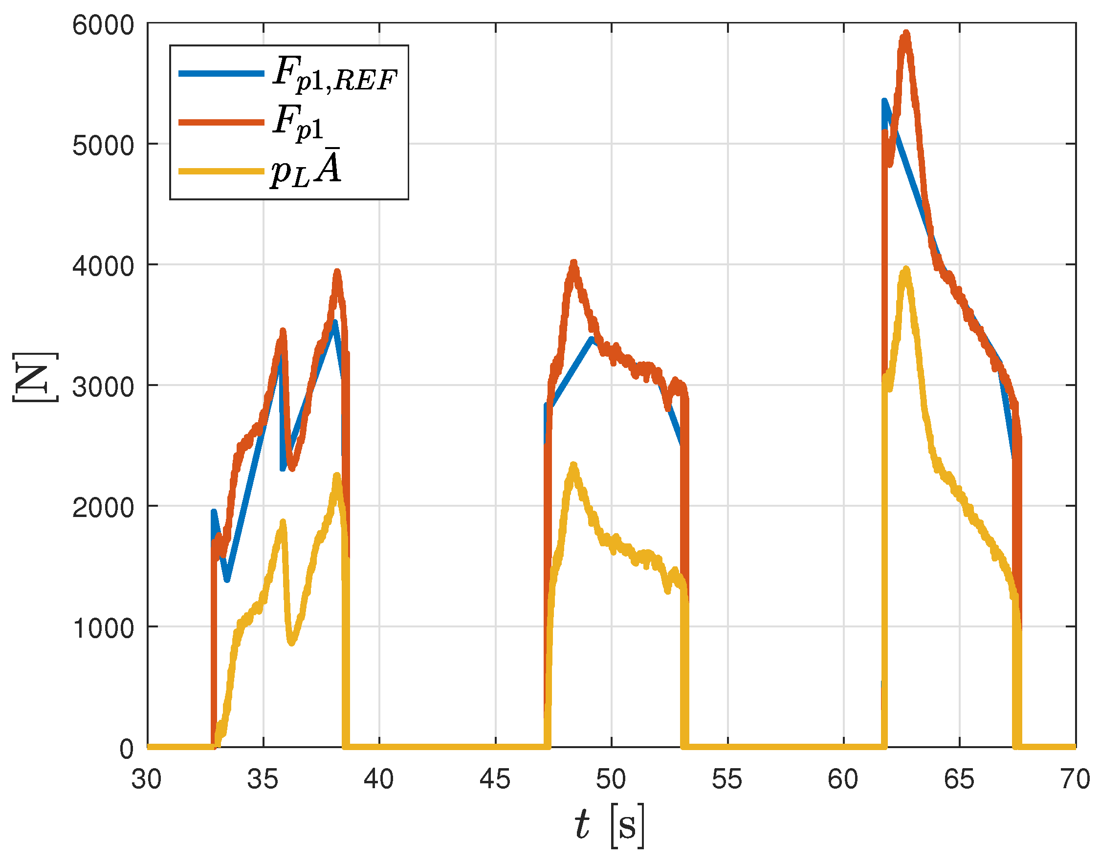
Figure 4 presents an example of pushing force setpoint tracking, where the external resistive force is modeled using the parameters ${\tau }_{ext}=0.002$ s, $F_{yield}=4000$ N.

It can be seen that the displayed resistive force qualitatively follows the typical stress profile during the material’s deformation, while the delay of the resistive force relative to the pushing force ensures the material’s change in momentum as long as the pushing force continues to increase.

2.1.3. Linearized Reduced-Order Actuator Model with External Force

The reduced-order model of a hydraulic actuator incorporating the proposed method for external force modeling can now be derived. This simplified model is crucial in forming the basis of the inversion-based feedforward control method.

Following standard practice [24,25], we introduce the load pressure as a measure of the actuation force,

$$p_L=p_A-p_B,$$

(14)

and the load flow (assuming $|Q_A|=|Q_B|$),

$$Q_L=Ku\sqrt{{\displaystyle \frac{1}{2}}\left(p_S-\mathrm{sign}\left(u\right)p_L\right)},$$

(15)

where K is the valve flow coefficient.

The chamber pressures can be expressed through the load pressure as follows (assuming zero pressure in the tank):

$$p_A={\displaystyle \frac{p_S+p_L}{2}},p_B={\displaystyle \frac{p_S-p_L}{2}}.$$

(16)

The load flow equation can be further simplified by linearizing it around an operating point $(\widehat{u},{\widehat{p}}_L)$:

$$Q_L={\widehat{Q}}_L+C_q(u-\widehat{u})-C_{qp}(p_L-{\widehat{p}}_L),$$

(17)

where

$$C_q={\displaystyle \frac{\partial Q_L}{\partial u}}{|}_{{\widehat{p}}_L}=K\sqrt{{\displaystyle \frac{1}{2}}\left(p_S-{\widehat{p}}_L\right)},$$

(18)

$$C_{qp}={\displaystyle \frac{\partial Q_L}{\partial p_L}}{|}_{\widehat{u}}=-{\displaystyle \frac{K\widehat{u}}{2\sqrt{2\left(p_S-{\widehat{p}}_L\right)}}}.$$

(19)

Equation (17) reduces to

$$Q_L=C_{q}u-C_{qp}(p_L-{\widehat{p}}_L),$$

(20)

because ${\widehat{Q}}_L=C_q\widehat{u}$.

If, instead of the analytical flow model (15), the flow curves provided by the manufacturer are used (as shown in Figure 1), it is necessary to utilize the full form of the linearized flow Equation (17) without prior simplification (20). Since this approach is also applied in the simulation model used in this study, the full form of the flow Equation (17) will be considered in the following text, with the coefficients $C_q$ and $C_{qp}$ determined numerically using the curves from Figure 1.

By applying these relations, the hydraulic continuity Equations (4) and (5) can be combined into a single equation related to the load pressure (neglecting leakage flows):

$$\dot{p_L}={\displaystyle \frac{4\beta }{V_t}}\left({\widehat{Q}}_L+C_q(u-\widehat{u})-C_{qp}(p_L-{\widehat{p}}_L)-\overline{A}v\right),$$

(21)

where $V_t$ is the total hydraulic actuator volume, $V_t=V_{A0}+V_{B0}$, and $\overline{A}$ is the average effective piston area, $\overline{A}=0.5(A_A+A_B)$.

Note that, for a symmetric actuator (double-rod cylinders), this approach is justified in calculating the actuation force as

$$F_{act}=p_L\overline{A}.$$

(22)

However, for non-symmetrical actuators, this method introduces an error due to the unequal surfaces of the piston. Despite this flaw, the advantages of this approach and its applicability to non-symmetrical actuators (which will be shown later) significantly outweigh the error. Therefore, we will use Equation (22) for the calculation of the actuation force in our reduced-order model.

The equation describing the change in external force over time can be considered under the reasonable assumption that the operating point is well above the pushing force threshold $F_{yield}$. Thus, based on Equations (11)–(13), the proposed model is reduced to

$${\dot{F}}_{ext}={\displaystyle \frac{1}{{\tau }_{ext}}}\left(F_p-F_{ext}\right).$$

(23)

Finally, the equation describing the motion of the piston retains its form described with Equation (1):

$$\dot{v}={\displaystyle \frac{1}{m}}\left(F_p-F_{ext}\right).$$

(24)

Combining Equations (23) and (24), one can obtain

$$v={\displaystyle \frac{{\tau }_{ext}}{m}}{F}_{ext}.$$

(25)

Now, we introduce a further simplification without loss of generality. Since, during force control operation, the cylinder piston moves continuously in one direction ($v>0$), a friction force model that does not consider the static component can be adopted, bypassing the issue with the $\mathrm{sign}(·)$ function:

$$F_{int}=\sigma v+F_{c0}.$$

(26)

Combining Equations (21), (23), and (25), and the fact that $F_p=p_L\overline{A}-F_{int}$, the following system of equations is obtained:

$${\dot{p}}_L={\displaystyle \frac{4\beta }{V_t}}\left({\widehat{Q}}_L+C_q(u-\widehat{u})-C_{qp}(p_L-{\widehat{p}}_L)-\overline{A}{\displaystyle \frac{{\tau }_{ext}}{m}}{F}_{ext}\right),$$

(27)

$${\dot{F}}_{ext}={\displaystyle \frac{1}{{\tau }_{ext}}}\left(p_L\overline{A}-\left(1+\sigma {\displaystyle \frac{\tau }{m}}\right)F_{ext}-F_{c0}\right).$$

(28)

For simpler notation, the previous equations can be written as follows:

$${\dot{p}}_L+C_1{p}_L=C_{2}u-C_3{F}_{ext}+C_7,$$

(29)

$${\dot{F}}_{ext}+C_4{F}_{ext}=C_5{p}_L-C_6,$$

(30)

where the introduced coefficients have the following values:

$$\begin{array}{cc}\hfill C_1& ={\displaystyle \frac{4\beta }{V_t}}{C}_{qp},C_2={\displaystyle \frac{4\beta }{V_t}}{C}_q,C_3={\displaystyle \frac{4\beta }{V_t}}\overline{A}{\displaystyle \frac{{\tau }_{ext}}{m}},\hfill \\ \hfill C_4& ={\displaystyle \frac{1}{{\tau }_{ext}}}+{\displaystyle \frac{\sigma }{m}},C_5={\displaystyle \frac{\overline{A}}{{\tau }_{ext}}},C_6={\displaystyle \frac{F_{c0}}{{\tau }_{ext}}},\hfill \\ \hfill C_7& ={\displaystyle \frac{4\beta }{V_t}}\left({\widehat{Q}}_L-C_q\widehat{u}+C_{qp}{\widehat{p}}_L\right).\hfill \end{array}$$

(31)

From Equation (29), $F_{ext}$ can be expressed and differentiated to obtain

$${\dot{F}}_{ext}={\displaystyle \frac{1}{C_3}}\left(C_2\dot{u}-{\ddot{p}}_L-C_1{\dot{p}}_L\right),$$

(32)

after which it can be inserted into Equation (30) to obtain

$${\displaystyle \frac{1}{C_3}}\left(C_2\dot{u}-{\ddot{p}}_L-C_1{\dot{p}}_L\right)+{\displaystyle \frac{C_4}{C_3}}\left(C_{2}u+C_7-{\dot{p}}_L-C_1{p}_L\right)=C_5{p}_L-C_6.$$

(33)

The notation can be further simplified by introducing coefficients

$$\begin{array}{cc}\hfill A_1& =C_1+C_4,A_0=C_5{C}_3+C_4{C}_1,\hfill \\ \hfill B_1& =C_2,B_0=C_4{C}_2,C=C_6{C}_3+C_4{C}_7.\hfill \end{array}$$

(34)

in order to obtain the final equation that relates the valve opening and the load pressure for the linearized reduced-order actuator model with the external force:

$${\ddot{p}}_L+A_1{\dot{p}}_L+A_0{p}_L=B_1\dot{u}+B_{0}u+C.$$

(35)

Figure 5 presents a comparison of the system’s response to a step valve opening obtained using a fully nonlinear simulation (mathematical model described in Section 2.1.1) and the reduced-order linearized model (35). For the operating point, the nominal values were determined and are shown in

Table 3. Nominal values for the operating point.

Parameter	Value
$\widehat{u}$	14 [%]
${\widehat{p}}_L$	20 [bar]
${\widehat{Q}}_L$	3.37 [L/min]
$C_q$	0.286634 [L/min/%]
$C_{qp}$	0.019195 [L/min/bar]

.

Figure 5 shows that using Equation (35) results in a slightly larger pushing force compared to the fully nonlinear model. This error is due to the linearization of the flow around the nominal point and the use of the reduced-order model. It should be noted that the accuracy of the model (35) improves as the surface areas on both sides of the cylinder piston become more similar. In reference [25], excellent agreement between the full and reduced-order hydraulic actuator models was achieved, but with a surface area ratio of 0.94. The cylinder considered in this study has a surface area ratio of 0.51, which is at the other extreme, making perfect agreement between the full and reduced models impossible.

From Figure 5, it can be seen that, for the nominal valve opening, the force calculation error is 33%, while, for smaller valve openings, it is 45%, and, for larger openings, it drops to 20%. This error arises from the reduced-order model’s inherent simplifications, particularly in the approximation of the load pressure using Equation (14). If this model were solely used for model-based control system synthesis—such as model predictive control (MPC) deployed on real hardware—these deviations would lead to degraded performance due to the missing dynamics and inaccuracies typical of reduced-order models. However, in the context of this study, the model is not intended to serve as the sole basis for control but rather as a component of a physics-guided neural network (PGNN)-based feedforward controller.

In a typical feedforward–feedback control structure, the feedforward component must generate the dominant part of the control signal to improve the system’s responsiveness. Since the feedforward signal in this study is composed of two parts—one derived from the reduced-order physical model and the other from a neural network correction term—the overall control signal accounts for discrepancies in the analytical model. The neural network component compensates for the reduced-order model’s limitations, particularly in regions where the approximation error is larger. Additionally, feedback control further refines the control signal, ensuring robustness even in operating conditions that deviate from the training set. Thus, despite the observed error levels in force prediction, the reduced-order model remains a suitable foundation for the proposed control architecture, as it provides a sufficiently accurate approximation of the system dynamics while enabling efficient PGNN-based correction.

2.2. Physics-Guided Neural Network-Based Feedforward Control

The core concept of the physics-guided neural network (PGNN) approach is to integrate the physical knowledge of the hydraulic actuator into a neural network-based feedforward control scheme. Rather than relying solely on data-driven methods or on purely model-based inversion, the PGNN combines both a reduced-order, physics-based model and a data-driven correction term. This synergy leverages physical laws for interpretability and robustness while using neural networks to compensate for nonlinearities and unmodeled effects.

In order to implement this PGNN-based feedforward controller effectively, it is essential to first formalize the control objective and describe the system dynamics. The objective of feedforward control is to compute the control input $u\left(k\right)$ such that the system output $y\left(k\right)$ follows a desired reference $r\left(k\right)$ with minimal error. Typically, the system dynamics can be represented using a nonlinear input–output model of the form

$$y\left(k\right)=h\left({[y(k-1),\dots ,y(k-n_a),u(k-n_k-1),\dots ,u(k-n_k-n_b)]}^T\right),$$

(36)

where $n_a$ and $n_b$ are the system order parameters, $n_k$ is the input delay, and $h(·)$ is an unknown nonlinear function. For ideal feedforward control, we assume the existence of an inverse model $h^{-1}(·)$, enabling the computation of the required input:

$$u_{\mathrm{ff}}\left(k\right)=h^{-1}\left({\varphi }_{\mathrm{ff}}\left(k\right)\right),$$

(37)

where the regressor vector ${\varphi }_{\mathrm{ff}}\left(k\right)$ includes future values of $r(·)$ and past inputs,

$${\varphi }_{\mathrm{ff}}\left(k\right)={\left[r(k+n_k+1),\dots ,r(k+n_k-n_a+1),u_{\mathrm{ff}}(k-1),\dots ,u_{\mathrm{ff}}(k-n_b+1)\right]}^T.$$

(38)

Due to the complexity of real-world systems, the inverse model $h^{-1}(·)$ is typically unknown or only partially known. To address this, the feedforward input $u_{\mathrm{ff}}\left(k\right)$ is decomposed into two components,

$$u_{\mathrm{ff}}\left(k\right)=f_{\mathrm{phy}}({\theta }_{\mathrm{phy}},\varphi \left(k\right))+g\left(\varphi \left(k\right)\right),$$

(39)

where $f_{\mathrm{phy}}({\theta }_{\mathrm{phy}},\varphi \left(k\right))$ is a reduced-order physics-based model that approximates the inverse dynamics, and $g\left(\varphi \right(k\left)\right)$ is the structural model error, accounting for the discrepancy between the true inverse model and the physics-based approximation.

The structural model error $g\left(\varphi \right(k\left)\right)$ can be defined as

$$g\left(\varphi \left(k\right)\right)=h^{-1}\left(\varphi \left(k\right)\right)-f_{\mathrm{phy}}({\mathit{\theta }}_{\mathrm{phy}},\varphi \left(k\right)).$$

(40)

This decomposition highlights the limitations of purely physics-based models in capturing system nonlinearities and motivates the introduction of data-driven methods to learn $g\left(\varphi \right(k\left)\right)$.

To capture these unmodeled dynamics, we introduce a physics-guided neural network (PGNN). Instead of relying solely on a data-driven network or a purely model-based approach, the PGNN combines both:

$$u_{\mathrm{ff}}\left(k\right)=f_{\mathrm{phy}}({\theta }_{\mathrm{phy}},\varphi \left(k\right))+f_{\mathrm{NN}}({\theta }_{\mathrm{NN}},T\left(\varphi \left(k\right)\right)),$$

(41)

where the term $f_{\mathrm{phy}}({\theta }_{\mathrm{phy}},\varphi \left(k\right))$ represents the physics-based model and captures the known dynamics of the system. The neural network component, $f_{\mathrm{NN}}({\theta }_{\mathrm{NN}},T\left(\varphi \left(k\right)\right))$, is trained to learn the residual dynamics or structural errors not captured by the physics-based model. The architecture of this hybrid approach is schematically illustrated in Figure 6.

We combine the unknown parameters into

$$\theta ={\left[{\theta }_{\mathrm{NN}}^T,{\theta }_{\mathrm{phy}}^T\right]}^T,$$

(42)

which includes the neural network weights ${\theta }_{\mathrm{NN}}$ and the physics-based model parameters ${\theta }_{\mathrm{phy}}$.

The input transformation $T\left(\varphi \left(k\right)\right):{\mathbb{R}}^{n_a+n_b}\to {\mathbb{R}}^{n_0}$ is optional and maps the input vector $\varphi \left(k\right)$ to a transformed space that improves the numerical properties and generates physically relevant features for the neural network. This transformation allows flexibility in defining the input features, such as normalizing the variables or incorporating additional physical insights. Such transformations often improve the numerical stability and training performance [16].

To address the challenge of overparameterization in the physics-guided neural network (PGNN) model and ensure physical interpretability during training, a regularized cost function is proposed [31]. The total cost function is defined as

$$V(\theta ,Z^N)=V_{\mathrm{MSE}}(\theta ,Z^N)+V_{\mathrm{reg}}\left(\theta \right),$$

(43)

where $V_{\mathrm{MSE}}(\theta ,Z^N)$ represents the mean squared error between the predicted and actual system outputs over the dataset $Z^N={\{\varphi \left[i\right],u\left[i\right]\}}_{i=1}^N$, and $V_{\mathrm{reg}}\left(\theta \right)$ is a regularization term designed to prevent competition between the physics-based and neural network layers.

The regularization term is formulated as

$$V_{\mathrm{reg}}\left(\theta \right):={∥\left[\begin{array}{cc}{\mathrm{\Lambda }}_{\mathrm{NN}}& 0\\ 0& {\mathrm{\Lambda }}_{\mathrm{phy}}\end{array}\right]\left(\theta -\left[\begin{array}{c}0\\ {\theta }_{\mathrm{phy}}^{\ast }\end{array}\right]\right)∥}_2^2,$$

(44)

where the term ${\theta }_{\mathrm{phy}}^{\ast }$ denotes the initial parameters of the physics-based model, typically obtained through system identification methods. The weighting matrices ${\mathrm{\Lambda }}_{\mathrm{NN}}$ and ${\mathrm{\Lambda }}_{\mathrm{phy}}$ control the relative importance of regularization for the neural network and physics-based components, respectively.

The purpose of the regularization term is twofold. First, it ensures that the neural network layer complements rather than overrides the physics-based model. Second, it prevents parameter drift in the physics-based layer, thereby preserving its interpretability and consistency with prior physical knowledge. Without regularization, the neural network may dominate the hybrid structure, leading to the loss of physical meaning and unstable behavior during training [16].

To determine the optimal parameter vector $\theta$ that best represents both the physics-based model and the residual dynamics captured by the neural network, we solve the following identification problem:

$$\widehat{\theta }=arg\underset{\theta }{min}V(\theta ,Z^N),$$

(45)

which emphasizes that the goal of the identification procedure is to find the optimal $\theta$ based on the available dataset $Z^N$.

The development of the PGNN-based feedforward controller begins with the reduced-order linearized actuator model derived in Section 2.1.3. This model approximates the inverse mapping from the desired output (e.g., the pushing force) and measurable states (e.g., load pressure) to the control input (valve opening).

To implement the controller in a digital form, the continuous time model is discretized. Starting from a linearized second-order equation such as (35), backward difference approximation is applied with a sampling period $T_s$. For the load pressure $p_L\left(k\right)$ and control input $u\left(k\right)$, this discretization leads to

$$\begin{array}{cc}\hfill {\displaystyle \frac{p_L\left(k\right)-2p_L(k-1)+p_L(k-2)}{T_s^2}}& +A_1{\displaystyle \frac{p_L\left(k\right)-p_L(k-1)}{T_s}}+A_0{p}_L\left(k\right)\hfill \\ \hfill & =B_1{\displaystyle \frac{u\left(k\right)-u(k-1)}{T_s}}+B_{0}u\left(k\right)+C,\hfill \end{array}$$

(46)

where $A_0$, $A_1$, $B_0$, $B_1$, and C are coefficients determined by linearization about the chosen operating point.

In practical implementations, the zero-order hold (ZOH) in the digital-to-analog converter introduces a half-sample ($T_s/2$) delay in $u\left(t\right)$. To compensate for this delay, all output dependencies are shifted forward by half a sample. Applying the shift operator $\Delta ={\displaystyle \frac{z+1}{2}}$ to (46) modifies the relationship, leading to new coefficients $A_0^{\prime },A_1^{\prime },A_2^{\prime },A_3^{\prime },B_0^{\prime },B_1^{\prime },$ and $D^{\prime }$. These coefficients, accounting for the shift, are defined as

$$\begin{array}{cc}\hfill A_0^{\prime }& =1+A_1{T}_s+A_0{T}_s^2,A_1^{\prime }=-1+A_1{T}_s+A_0{T}_s^2,\hfill \\ \hfill A_2^{\prime }& =-1-A_1{T}_s+A_0{T}_s^2,A_3^{\prime }=1-A_1{T}_s+A_0{T}_s^2,\hfill \\ \hfill B_0^{\prime }& =2T_s{B}_1+2T_s^2{B}_0,B_1^{\prime }=-2T_s{B}_1,D^{\prime }=2T_s^{2}C.\hfill \end{array}$$

(47)

Using these new coefficients, the discretized system equation is expressed as

$$\begin{array}{c}\hfill A_0^{\prime }{p}_L[k+1]+A_1^{\prime }{p}_L\left[k\right]+A_2^{\prime }{p}_L[k-1]+A_3^{\prime }{p}_L[k-2]=B_0^{\prime }u\left[k\right]+B_1^{\prime }u[k-1]+D^{\prime }.\end{array}$$

(48)

Solving for $u\left[k\right]$ leads to an expression of the form

$$u\left[k\right]={\theta }_{\mathrm{phy}}^{\top }\varphi \left[k\right],$$

(49)

where ${\theta }_{\mathrm{phy}}$ is a parameter vector containing the identified physical parameters from Equation (47), and

$$\varphi \left[k\right]={\left[\begin{array}{cccccc}{p}_L[k+1]& p_L\left[k\right]& p_L[k-1]& p_L[k-2]& u[k-1]& 1\end{array}\right]}^{\top }$$

(50)

is the regressor vector constructed from past outputs and inputs.

2.3. Experimental Setup

The piercing process is inherently complex from the control system synthesis perspective, as it involves the coordination of multiple controllers with different functions. For instance, during a single work cycle of the two cylinders, the following sequence takes place.

• Initially, one cylinder operates in force mode, maintaining a constant pressing force on the material.
• As the first cylinder approaches the end of its stroke, the second cylinder begins to move, matching the speed of the first to ensure a smooth transition of force.
• During the overlap, when both grippers are active, both cylinders operate in force mode, providing a constant resultant force, as illustrated in Figure 7.
• Once the force has fully transitioned to the second cylinder, the first cylinder’s gripper is deactivated, and the first cylinder returns to its starting position.

Figure 7. Force exchange between two cylinders during material pressing into the mill.

Figure 7. Force exchange between two cylinders during material pressing into the mill.

This cycle then repeats with the roles of the two cylinders reversed. Consequently, for the successful execution of each sequence, and thus the entire continuous process, it is critical to coordinate three control subsystems: force, speed, and position control.

However, since the objective of this paper is to investigate the application of different feedforward strategies based on neural networks within the force control subsystem, the other two control subsystems—position and velocity—will not be addressed here.

The schematic structure of the force control system for one cylinder is presented in Figure 8.

The control system is configured as a PI regulator with feedforward, where the feedforward component, in general, determines the dominant part of the control signal based on the desired force and the current piston speed. The role of the PI controller is to correct minor deviations from the force setpoint, generating the remaining portion of the control signal.

The feedback signal for the force controller, as well as the measured piston velocity for the feedforward, are obtained from pressure sensors in the cylinder chambers and the position sensor of the piston, respectively. The control signal is provided as the desired opening of the proportional 3/4 directional control valve (DCV).

In Figure 8, the feedforward is represented by a neural network symbol with two inputs: the desired force and the actual velocity. This feedforward structure corresponds to the benchmark model described in Section 3.1.1. When using the PGNN, the structure of the feedforward neural network differs, as its inputs depend not only on the current desired force but also on its previous values and the previous outputs of the network, as shown in Figure 6. Since this recurrent connection is internal to the PGNN, it is not explicitly shown in Figure 8 for simplicity. However, compared to the benchmark model, the key difference is that the PGNN does not require the current velocity value to generate its portion of the control signal.

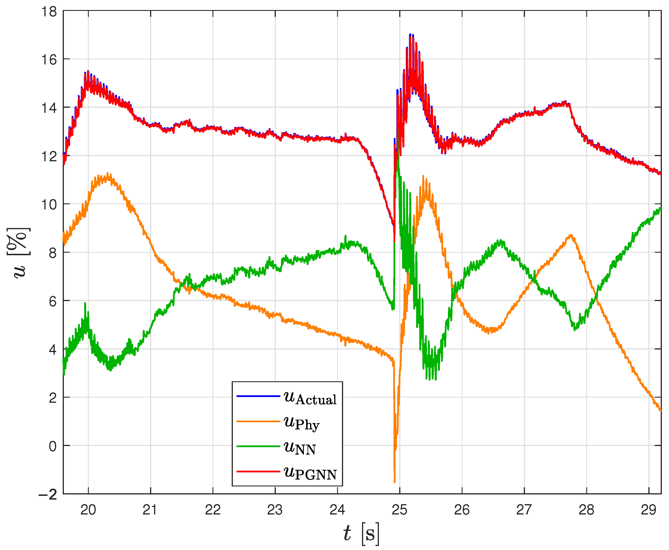
To implement the PGNN, the desired pushing force, $F_{p,\mathrm{DES}}$, is divided by the average piston surface area, $\overline{A}$, to compute the desired load pressure, $p_L$, which serves as an input to the PGNN. This load pressure, $p_L$, is used to form the input regressor vector, allowing the PGNN to capture the system’s dynamics. Furthermore, since the reference force is known in advance, the PGNN can utilize information about previous inputs, previous outputs, and future values of $p_L$ to generate precise predictions.

By managing the recurrent connection internally, as depicted in Figure 6, the PGNN effectively models dependencies on previous states and outputs, enabling it to predict the required valve opening with high accuracy.

For the purposes of testing and synthesizing the control system for the seamless pipe manufacturing process from a continuously cast material, a scaled-down model of the entrance device was developed, as shown in Figure 9. This model consists of an electro-hydraulic system with two cylinders, grippers, control valves, a pump unit, a reservoir, and accompanying electronics to implement the methods discussed in this paper.

The control system depicted in Figure 8 has been implemented using a Siemens S7-1517T PLC, which includes a neural processing unit (NPU) module for real-time neural network evaluation. The PLC acts as the system’s central controller, managing the primary control loops, such as the PID-based force regulation. It also handles sensor inputs (e.g., pressure transducers) and actuator outputs (e.g., valve control). The PLC interfaces with distributed sensors and actuators via PROFINET, connected to an ET 200S I/O station for efficient field-level communication. To control the hydraulic cylinders, the SimaHydTO library [32] is employed, offering modular function blocks for precise position and force control. This library also facilitates real-time monitoring and compensation for valve nonlinearities. While a technology CPU is not required for most basic motion operations, it is essential for advanced synchronization tasks such as camming and cam track operations.

The PGNN is executed on the technology module neural processing unit (TM NPU), which is powered by the AI-capable Intel Movidius Myriad X processing unit. The NPU contains two LEON CPUs and 16 SHAVE parallel processors, capable of accelerating neural networks in hardware, with a peak compute capacity of up to 4 TOPs [33]. As shown in Figure 10, data exchange between the PLC and NPU occurs over the backplane bus, enabling real-time communication. In our setup, the execution time for the neural network within the NPU was approximately 650 $\mathsf{\mu }$s, with data transfer between the PLC and NPU occurring at intervals of 4 ms.

3. Results

3.1. Neural Network Training

In this section, we present the results of two neural network-based frameworks for the feedforward controller training process. For the benchmark model, a neural network trained on data collected from tests with various piston speeds and actuation forces is employed, which is an experimentally intensive process. To overcome this challenge, the training results of a physics-guided neural network are presented, incorporating our reduced-order actuator model for feedforward control, which is far less dependent on extensive training data.

3.1.1. Benchmark Neural Network

The core concept of this benchmark model is to calculate the necessary valve opening based on the current piston speed and the desired actuation force.

To establish this relationship, the following test setup is proposed.

• Both grippers (Figure 3) are engaged, creating a rigid mechanical connection between the two pistons.
• The first cylinder operates in velocity mode, moving at a constant speed.
• The second cylinder operates in force mode, simulating resistance to the movement of the first cylinder.
• Experiments are conducted for the relevant ranges of piston speeds and forces.

The basic idea is to train the network on the relevant dataset to achieve the high-quality approximation of the velocity–force characteristics of the actuation system.

Table 4. Valve opening for different force and piston velocity values. Only the part of the dataset used to train the benchmark neural network is presented. The complete dataset is provided in the Supplementary Materials (BenchmarkNeuralNetwork_Dataset).

Force [kN]	Piston Velocity [mm/s]
	10	20	30	40	50
1	3.982	6.882	9.782	12.682	15.582
2	4.062	6.962	9.862	12.762	15.662
3	4.142	7.042	9.942	12.842	15.742
4	4.222	7.122	10.022	12.922	15.822
5	4.302	7.202	10.102	13.002	15.902
6	4.382	7.282	10.182	13.082	15.982
7	4.462	7.362	10.262	13.162	16.062

presents the achieved valve opening for different force values and a few characteristic piston velocities. The complete dataset used to train the benchmark neural network is provided in the Supplementary Materials (BenchmarkNeuralNetwork_Dataset). It should be noted that the data arrangement in the Supplementary Materials is the same as in Table 4, i.e., the first column contains the force values, the first row lists the velocities, and the rest of the table consists of the valve opening values for each force–velocity combination.

Considering the need for the real-time implementation of the neural network, a relatively simple network structure was selected.

• Two inputs: actual piston speed [mm/s] and desired force [kN].
• Two hidden layers with 32 nodes each.
• ReLU activation functions.
• One output: valve opening [%].

To train the network, the Levenberg–Marquardt backpropagation algorithm [34] was used, with the training parameters shown in

Table 5. Training parameters for the benchmark neural network.

Parameter	Value
Minimum Gradient	1 × 10−7
$\mu$	0.001
$\mu$ Decrease Ratio	0.1
$\mu$ Increase Ratio	10

.

Figure 11 illustrates the training process, showing the loss curve over 500 epochs, which was found to be sufficient as the network achieved a validation result of 2.2147 × 10${-}^9$, indicating an extremely low error rate and a highly accurate model fit.

3.1.2. Physics-Guided Neural Network Training

For the creation of the training dataset for the PGNN, the setup was slightly modified compared to the training of the benchmark model.

• Both grippers (Figure 3) are engaged, creating a rigid mechanical connection between the two pistons.
• The first cylinder operates in force mode, following the desired force value ramps, using any type of controller. The term “any” is used here because the quality of tracking of the desired force value is not crucial in generating the training dataset; rather, the focus is on covering the entire operating range of interest. For our purposes, a simple PI controller without feedforward is used, with initially selected gains that are not thoroughly tuned.
• The second cylinder operates in velocity mode, moving at a constant speed, which is selected as the expected insertion speed of the material into the mill during the process.
• Since the cylinder stroke is limited, and to ensure that the training set is sufficiently rich, when the piston reaches its fully extended position, the second cylinder is commanded to move at a negative speed until it reaches the fully retracted position, after which it is again assigned a positive speed. This cycle is repeated as many times as necessary, depending on the desired dataset size, sampling frequency, and piston speed in the operating regime.
  During the return of the pistons to the starting position, there is no need to change the operating mode of the first cylinder. It is only necessary to ensure that the reference signal for the force ramps, which the first cylinder is supposed to follow, is sufficiently large and randomized to avoid repetition during the experiments.

It is important to note that, in order for the training dataset to align with the physical part of the PGNN, as mathematically described in Section 2.1.3, specifically due to the assumption of continuous motion and the absence of static friction and signum issues, only the portions of the recorded data corresponding to positive piston speeds are adopted for the final training set.

An example of such a dataset is shown in Figure 12, covering three consecutive positive movements. The portion of the recorded data corresponding to negative speeds is not displayed. The sampling frequency was set to 250 Hz, and, for a cylinder stroke of 340 mm and a speed of 40 mm/s, one positive movement corresponds to a set of approximately 8 s.

In Figure 12, alongside the desired and actual force values, the value of $p_L\overline{A}$ is also displayed, which corresponds to the force calculated using the linearized reduced-order model, represented by Equation (22). Similar behavior to that seen in Figure 5 or the simulation model is observed. Specifically, for lower force values, the error of the linearized reduced-order model is significant, while, with increasing force, the reduced model provides a closer approximation of the real system.

This is shown in Figure 13, where the force calculation error of the linearized reduced-order model falls to nearly 30%. This error primarily results from the linearization process and the use of a reduced-order model, which estimates the force based on the load pressure and an average effective piston area. A more accurate force prediction would require piston surface areas that are more similar, with the extreme case being a double-rod cylinder where the area ratio is 1. However, in this study, the reduced-order model is not expected to provide an exact force calculation but rather to generate the dominant portion of the feedforward control signal. The remaining part is corrected by the neural network component of the PGNN, which is trained on these data to compensate for modeling errors. Additionally, the feedback loop further refines the control signal, ensuring overall robustness. Thus, despite the 30% error in the physical model, this deviation is deemed acceptable because it is the task of the PGNN to minimize it by integrating the neural network component with the physical model.

Figure 14 and Figure 15 display the achieved valve opening values, concentrated around a nominal value of 14%, and the piston speed, respectively, again only for positive movement speeds.

The dataset used to train the PGNN consists of measurements of the load pressure, $p_L$, and the control signal, u. As described in Equation (50), the regressor vector is constructed for each time index k. This regressor vector (or, equivalently, the input vector) is used as input to the PGNN.

To ensure proper numerical conditioning, the regressor vector is processed in two segments. The first four components (i.e., the load pressure measurements) are standardized via z-score normalization using scikit-learn’s StandardScaler. In contrast, the fifth component, corresponding to the previous control signal $u[k-1]$, and the target output $u\left[k\right]$ are normalized using min–max scaling to the interval $[0,1]$ because u is naturally bounded between 0% and 100%. The constant term (the sixth component) remains unscaled. All scaling parameters (means, standard deviations, minimum, and range) are computed solely from the training set (70% of the data) and then applied to both the training and validation sets (the remaining 30%).

The proposed PGNN architecture is composed of two distinct parts. The first part is a fixed physical model layer, implemented as a custom, non-trainable layer in TensorFlow. Its role is to capture the dominant system dynamics by computing

$$u_{\mathrm{phy}}={\theta }_{\mathrm{phy}}^{\ast \top }\varphi \left[k\right],$$

(51)

where ${\theta }_{\mathrm{phy}}^{\ast }$ are the initial parameters from Equation (48). Because the data are scaled prior to training, the physical model parameters must be adjusted accordingly. Let S denote the vector of scaling factors (standard deviations for the first four components and the range for the fifth component) and m the vector of corresponding offsets (means for the first four components and the minimum for the fifth component). If the control signal is normalized via min–max scaling with minimum $u_{min}$ and range $u_{\mathrm{range}}=u_{max}-u_{min}$, the adjusted parameters are computed as

$${\theta }_{\mathrm{phy},\mathrm{adjusted}}={\displaystyle \frac{{\theta }_{\mathrm{phy}}^{\ast }\odot S}{u_{\mathrm{range}}}},b_{\mathrm{phy}}={\displaystyle \frac{{\theta }_{\mathrm{phy}}^{\ast \top }m-u_{min}}{u_{\mathrm{range}}}},$$

(52)

where “⊙” denotes element-wise multiplication. This layer is embedded in the PGNN and remains fixed during training, thereby preserving the physical interpretability.

The second part of the PGNN is a trainable neural network correction branch. This branch comprises two hidden layers with 16 neurons each and hyperbolic tangent activation functions. Its output, denoted by $u_{\mathrm{NN}}$, provides a correction term that compensates for discrepancies between the physical model and the true inverse dynamics. The overall PGNN output is obtained as the sum

$$\widehat{u}\left[k\right]=u_{\mathrm{phy}}+u_{\mathrm{NN}},$$

(53)

which is then mapped back to the original units via the inverse min–max transformation.

During training, the dataset is divided into 70% for training and 30% for validation. The PGNN is trained using the Adam optimizer (with a learning rate of 0.001) over 70 epochs with a batch size of 32. A custom loss function, defined with Equation (43), is used during training, with a slight modification to the regularization term:

$$V_{\mathrm{reg}}\left(\theta \right)={\lambda }_{\mathrm{NN}}\sum _{w\in {\mathcal{W}}_{\mathrm{NN}}}{\parallel w\parallel }^2.$$

(54)

Here, ${\mathcal{W}}_{\mathrm{NN}}$ denotes the set of weights in the neural network correction branch. The $L_2$ regularization is applied solely to these weights, while leaving the physical model layer parameters fixed. We set ${\lambda }_{\mathrm{NN}}=1\times {10}^{-5}$; this small value was chosen empirically to provide sufficient regularization to prevent overfitting, while allowing the correction branch to effectively learn the residual dynamics.

Figure 16 shows the convergence of the training and validation loss curves, which demonstrates the effective generalization of the PGNN. For comparison, a standalone neural network with two hidden layers of 32 neurons each (and the same activation functions) was also implemented; this network lacks the physics-based constraints and requires a larger dataset to achieve similar performance.

The identified physical model, obtained using least squares system identification, serves as a baseline. While it achieves reasonable accuracy, the estimated parameters often lack physical interpretability, limiting their application under new conditions. In contrast, the standalone neural network achieves similar accuracy but requires larger datasets and lacks physical interpretability, making it less robust in scenarios with limited data availability.

Figure 17 highlights the PGNN’s decomposition into contributions from the physical model (orange line) and the neural network correction (green line). The total PGNN output (red line) closely matches the actual system behavior (blue line), demonstrating the synergy between the physics-based model and the neural network correction.

A performance comparison of the PGNN, standalone neural network, and physical models is shown in Figure 18, with the quantitative results summarized in

Table 6. MSE in % for different models in Figure 18.

Model	Physical Model (ID)	Standalone NN	PGNN
MSE (%)	$2.49·{10}^{-2}$	$2.42·{10}^{-2}$	$2.33·{10}^{-2}$

. The PGNN achieves the lowest MSE among the models. By embedding physical constraints and leveraging data-driven corrections, the PGNN outperforms the standalone approaches in scenarios with an incomplete physical understanding or limited data.

3.2. Final Experiments

3.2.1. Constant Setpoint Tracking with Benchmark Neural Network

The first experiment was chosen to verify the applicability of the benchmark neural network in real time and its integration with the existing controller structure on the PLC.

In this experiment, a comparison was performed with a force PI controller, which is the standard type of controller for this application in industrial settings. It is important to note that, when using the benchmark neural network to compute the feedforward part of the control signal, the feedback component remains present in the form of a PI controller to ensure overall robustness in real industrial applications.

The test setup was as follows.

• Both grippers (Figure 3) are engaged, creating a rigid mechanical connection between the two pistons.
• The first cylinder operates in force mode, following a constant setpoint for the pushing force (1000 N).
• The second cylinder operates in velocity mode, tracking step changes in speed. Due to the limited stroke of the cylinder, and to cover a wide range of speeds during a single stroke, the durations at specific speeds are kept short, resulting in a speed profile, as shown in Figure 19, that resembles a linear change in velocity.

Although the system is designed to operate at approximately constant speeds and forces, this experiment was selected with the aim to test the response of the cylinder, maintaining a constant force, to disturbances in the form of speed variations generated by the second cylinder.

The speed range covered was from 0 to 20 mm/s, and, to gain insights into the advantages of using a neural network as a feedforward, the same desired speed profile was requested from the second cylinder during both tests, with and without the feedforward. The speeds achieved during the tests are shown in Figure 19, where it can be observed that the speed profile was approximately the same during both experiments.

Figure 19. Piston speeds during constant setpoint tracking, with different controller structures: PI controller; benchmark neural network feedforward.

Figure 19. Piston speeds during constant setpoint tracking, with different controller structures: PI controller; benchmark neural network feedforward.

Figure 20 presents a comparative analysis of the results for the maintenance of a constant force setpoint in the presence of velocity disturbances, both with and without the feedforward. In the first case, a standard PI controller was used, while, in the second case, the benchmark neural network acted as the feedforward, determining the dominant part of the control signal based on the desired force value and the current speed.

The fluctuations around the desired force value, as a result of the continuously increasing piston speed, are clearly visible in Figure 20. However, the improved tracking of the desired value can be observed when the neural network-based feedforward is used. This improvement can also be quantified by the integral of the squared error (ISE), which, in the mentioned cases, amounts to

$${\left(\mathrm{ISE}\right)}_{\mathrm{PI}}=150.44,{\left(\mathrm{ISE}\right)}_{\mathrm{Benchmark}\mathrm{NN}}=134.75$$

Figure 21 shows the calculated control signal for the experiment with the benchmark neural network-based feedforward. Since this controller includes both the feedforward and feedback components, the figure presents the total control output, as well as the portion of the control signal generated by the neural network through the feedforward path, on the NPU device. It can be observed that the neural network output closely follows the trend of the piston speed changes.

In this experiment, we demonstrated that the neural network, with a structure that is complex enough to capture the nonlinear characteristics of the hydraulic actuator, can be successfully implemented on a neural processing unit. It provides a fast response to sudden changes in the operating conditions, proving its effectiveness in real-time applications and making it a relevant benchmark for the evaluation of the PGNN in the next experiment.

3.2.2. Varying Setpoint Tracking with Different Feedforward Structures

The second experiment was chosen with the aim of comparatively demonstrating the application of different feedforward structures in real time under conditions that correspond to operational use. The test setup was as follows.

• Both grippers (Figure 3) are engaged, creating a rigid mechanical connection between the two pistons.
• The first cylinder operates in force mode, following a ramp setpoint for the pushing force, with a randomized profile within the operational force range.
• The second cylinder operates in velocity mode, maintaining a constant speed of approximately 40 mm/s, which corresponds to the operating conditions of the real system.

Three control system structures were tested:

• A PI controller without feedforward;
• A PI controller with neural network-based feedforward that has access to both speed and desired force information (benchmark neural network feedforward);
• A PI controller with a physics-guided neural controller with neural network-based feedforward that has access only to the desired force (PGNN feedforward).

Figure 22 presents a comparative analysis of the force ramp tracking using the three controllers mentioned. It is evident that the use of the PI controller alone is insufficient in tracking the time-varying reference signal.

As seen in the figure, both feedforwards result in the good tracking of the desired force value, except in the section where the reference value begins to decrease. This indicates that the PI controller’s gains are not optimally tuned in the presence of the feedforward, with their high values leading to overshoot.

Nevertheless, the use of both feedforwards resulted in good setpoint tracking, with the following integral of the squared error values for the part of the experiment shown in Figure 22:

$${\left(\mathrm{ISE}\right)}_{\mathrm{PI}}=20.3985,{\left(\mathrm{ISE}\right)}_{\mathrm{Benchmark}\mathrm{NN}}=3.9848,{\left(\mathrm{ISE}\right)}_{\mathrm{PGNN}}=3.6953$$

It is important to note how the PGNN-based feedforward compares to the benchmark network, which is significantly more training-demanding.

The final output of the system is also influenced by the quality of the second cylinder’s tracking of the desired velocity. Given the mechanical connection between the cylinders, there is a mutual influence between them, even though they operate in different modes (force and velocity). The achieved velocity profile during the observed part of the experiment is shown in Figure 23.

It is observed that the quality of the tracking of the desired velocity is somewhat lower; however, it should be noted that velocity regulation was not the focus of this work. The task of the second cylinder was to provide an approximate expected velocity during the production process, without strict requirements regarding oscillations and steady-state errors. Furthermore, as previously mentioned, from the perspective of the force control system of the first cylinder, the variable motion represents a disturbance that must be addressed by maintaining the desired force. Therefore, the variable motion of the entire system during the experiment supports the examination of the robustness of the force controller.

4. Discussion

In this paper, a detailed methodology for the application of neural networks for feedforward control to a specific manufacturing process—seamless pipe production—was developed.

Starting from the general nonlinear model of a hydraulic cylinder, used as an actuator in this industrial process, the unknown parameters of the mathematical model were identified. Although, in the realm of neural networks, precise knowledge of the system parameters is often unnecessary due to their universal approximator nature, this work emphasizes parameter identification as a step toward embedding knowledge of the dynamic system into the artificial intelligence workflow.

Of course, neural networks could also have been used for the identification of the unknown parameters of the hydraulic actuator, as extensively covered in the existing literature [26]. However, such an approach would compromise the interpretability and the possibility of further simplifying the mathematical model—an essential step in coupling physical models with neural networks.

It was demonstrated that, by using traditional identification methods, such as the least squares method, and based on straightforward experiments on real hardware (cylinder responses to step changes in valve openings), it is possible to determine unknown parameters with sufficient accuracy to capture the dominant system dynamics.

Processes in heavy industry, such as seamless pipe manufacturing, are distinct from the perspective of control system synthesis due to the coupling between the dynamics of the actuators and the working material or the process itself. Therefore, to fully capture the system’s dynamics, regardless of the required accuracy, it is essential to adopt a mathematical model that encompasses this interaction. We propose that such a model should be sufficiently rich to capture the phenomena that predominantly influence the controlled system, yet simple enough to preserve the concept of physical models that can be seamlessly integrated with neural networks.

In this particular task, the dominant factors by which the production process influences the actuator’s operation are friction and the behavior of the cast material under deformation. Therefore, this paper proposes a model of external force defined by two parameters: the pushing force threshold $F_{yield}$ and the time constant ${\tau }_{ext}$. These parameters can be identified using experimentally recorded data from the existing production process.

A potential direction for future work could focus on the application of neural networks to emulate the material being pressed into the piercing mill. This approach would be beneficial as it would enable the simulation of the workpiece’s impact using simplified hardware, such as the example of two coupled cylinders—one responsible for pushing the material and the other simulating the resistive force—thus allowing the control system to be tuned outside the industrial environment.

With the finalized mathematical model of the entire production process, it becomes possible to proceed with its simplification as a preparation step for the formation of inversion-based models. The process model, represented by Equation (35), was derived using a reduced-order model of the hydraulic cylinder [25] and adopting justified assumptions specific to this production process: unidirectional material movement and a velocity high enough to neglect the static component of friction.

It has been shown that the deviations resulting from the use of the reduced hydraulic cylinder model are around 30%, within the expected operating point range, which would lead to significant discrepancies if the obtained inversion-based model were the sole method used in generating the control signal. However, since one of the primary objectives of this work was the integration of physical models into the structure of neural networks to enable their safer and more predictable industrial application, the obtained inversion-based models are responsible only for generating a portion of the control signal through the feedforward. The remaining part of the feedforward control signal is generated by a neural network, facilitated by the recently introduced concept of physics-guided neural networks [16].

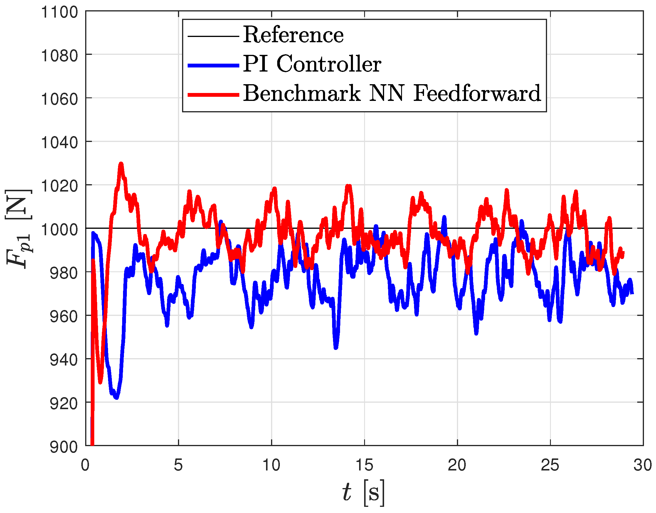
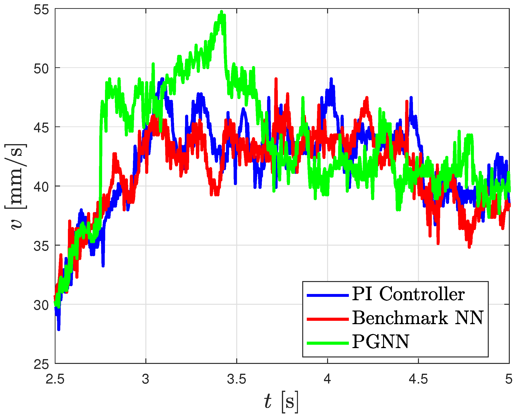
Although the advantages of PGNNs have, so far, primarily been demonstrated through comparisons between PGNN-based feedforwards and feedforwards based on purely neural networks, both trained on the same dataset collected from real machines, in our work, PGNNs are compared with feedforward based on a richer-structured neural network that includes also the material velocity as an input, which we refer to as the benchmark neural network. Both the PGNN and our benchmark NN were trained using experimental data collected from a real machine—the entrance device simulator. It was demonstrated that the PGNN, requiring significantly fewer experiments, with only a few passes through the cylinder’s working stroke—was comparable to the benchmark neural network, which required extensive data collection across the entire range of speeds and forces for training.

The focus throughout this work was on finding a feedforward structure that provides a sufficiently detailed description of the system behavior, incorporates the physicality of the process to prevent the control variables from exceeding the expected values for the chosen operating point, and remains simple enough for all computations to be performed in real time. For this reason, all experiments were conducted on real hardware, using standard modules available for industrial applications. It has been demonstrated that the currently available neural processing units are suitable for the implementation of physics-guided neural networks.

Such structured control systems enable the safer integration of artificial intelligence methods into industrial processes compared to traditional neural network-based feedforwards. This is because embedded physical models generate the dominant portion of the control signal, even under operating conditions for which the neural network was not trained. This is a common scenario in industrial processes, where the training of the network must often be performed on a limited dataset.

References

1. Erman, E. The influence of the processing parameters on the performance of the two-roll piercing operation. J. Mech. Work. Technol. 1987, 15, 167–179. [Google Scholar] [CrossRef]
2. Parshin, V.M.; Smolyakov, A.S.; Khrebin, V.N.; Zhikharev, P.Y. Production of hollow continuous-cast billet for seamless pipe. Steel Transl. 2012, 42, 825–829. [Google Scholar] [CrossRef]
3. Devasia, S. Should model-based inverse inputs be used as feedforward under plant uncertainty? IEEE Trans. Autom. Control 2002, 47, 1865–1871. [Google Scholar] [CrossRef]
4. van Zundert, J.; Oomen, T. On inversion-based approaches for feedforward and ILC. Mechatronics 2018, 50, 282–291. [Google Scholar] [CrossRef]
5. Boerlage, M.; Steinbuch, M.; Lambrechts, P.; van de Wal, M. Model-based feedforward for motion systems. In Proceedings of the 2003 IEEE Conference on Control Applications, Istanbul, Turkey, 25 June 2003; Volume 2, pp. 1158–1163. [Google Scholar] [CrossRef]
6. Devasia, S. Iterative Machine Learning for Output Tracking. IEEE Trans. Control Syst. Technol. 2019, 27, 516–526. [Google Scholar] [CrossRef]
7. Butterworth, J.; Pao, L.; Abramovitch, D. Analysis and comparison of three discrete-time feedforward model-inverse control techniques for nonminimum-phase systems. Mechatronics 2012, 22, 577–587. [Google Scholar] [CrossRef]
8. Schoukens, J.; Ljung, L. Nonlinear System Identification: A User-Oriented Road Map. IEEE Control Syst. Mag. 2019, 39, 28–99. [Google Scholar] [CrossRef]
9. Hornik, K.; Stinchcombe, M.; White, H. Multilayer feedforward networks are universal approximators. Neural Netw. 1989, 2, 359–366. [Google Scholar] [CrossRef]
10. Sørensen, O. Additive feedforward control with neural networks. IFAC Proc. Vol. 1999, 32, 1378–1383. [Google Scholar] [CrossRef]
11. Li, G.; Na, J.; Stoten, D.P.; Ren, X. Adaptive Neural Network Feedforward Control for Dynamically Substructured Systems. IEEE Trans. Control Syst. Technol. 2014, 22, 944–954. [Google Scholar] [CrossRef]
12. Hunt, K.; Sbarbaro, D.; Żbikowski, R.; Gawthrop, P. Neural networks for control systems—A survey. Automatica 1992, 28, 1083–1112. [Google Scholar] [CrossRef]
13. Ljung, L.; Andersson, C.; Tiels, K.; Schön, T.B. Deep Learning and System Identification. IFAC PapersOnLine 2020, 53, 1175–1181. [Google Scholar] [CrossRef]
14. Raissi, M.; Perdikaris, P.; Karniadakis, G. Physics-informed neural networks: A deep learning framework for solving forward and inverse problems involving nonlinear partial differential equations. J. Comput. Phys. 2019, 378, 686–707. [Google Scholar] [CrossRef]
15. Bolderman, M.; Fan, D.; Lazar, M.; Butler, H. Generalized feedforward control using physics—informed neural networks. IFAC PapersOnLine 2022, 55, 148–153. [Google Scholar] [CrossRef]
16. Bolderman, M.; Butler, H.; Koekebakker, S.; van Horssen, E.; Kamidi, R.; Spaan-Burke, T.; Strijbosch, N.; Lazar, M. Physics-guided neural networks for feedforward control with input-to-state-stability guarantees. Control Eng. Pract. 2024, 145, 105851. [Google Scholar] [CrossRef]
17. Fan, D.; Bolderman, M.; Koekebakker, S.; Butler, H.; Lazar, M. Physics–guided neural networks for inversion–based feedforward control applied to hybrid stepper motors. In Proceedings of the 2023 IEEE Conference on Control Technology and Applications (CCTA), San Diego, CA, USA, 9–11 August 2023; pp. 1153–1158. [Google Scholar] [CrossRef]
18. Kon, J.; de Vos, N.; Bruijnen, D.; van de Wijdeven, J.; Heertjes, M.; Oomen, T. Learning for Precision Motion of an Interventional X-ray System: Add-on Physics-Guided Neural Network Feedforward Control. IFAC PapersOnLine 2023, 56, 7523–7528. [Google Scholar] [CrossRef]
19. Bolderman, M.; Lazar, M.; Butler, H. Structured physics-guided neural networks for electromagnetic commutation applied to industrial linear motors. Mechatronics 2025, 106, 103291. [Google Scholar] [CrossRef]
20. Ahmad, B.; Prajitno, P. Design of neural network and PLC-based water flow controller. J. Phys. Conf. Ser. 2020, 1528, 012065. [Google Scholar] [CrossRef]
21. Solowjow, E.; Ugalde, I.; Shahapurkar, Y.; Aparicio, J.; Mahler, J.; Satish, V.; Goldberg, K.; Claussen, H. Industrial Robot Grasping with Deep Learning using a Programmable Logic Controller (PLC). In Proceedings of the 2020 IEEE 16th International Conference on Automation Science and Engineering (CASE), Hong Kong, China, 20–21 August 2020. [Google Scholar]
22. Rybczak, M.; Popowniak, N.; Kozakiewicz, K. Applied AI with PLC and IRB1200. Appl. Sci. 2022, 12, 12918. [Google Scholar] [CrossRef]
23. Schmidt, A.; Schellroth, F.; Fischer, M. Reinforcement learning methods based on GPU accelerated industrial control hardware. Neural Comput. Appl. 2021, 33, 12191–12207. [Google Scholar] [CrossRef]
24. Jelali, M.; Kroll, A. Physically Based Modelling. In Hydraulic Servo-Systems: Modelling, Identification and Control; Springer: London, UK, 2003; pp. 53–126. [Google Scholar] [CrossRef]
25. Ruderman, M. Full- and reduced-order model of hydraulic cylinder for motion control. In Proceedings of the IECON 2017—43rd Annual Conference of the IEEE Industrial Electronics Society, Beijing, China, 29 October–1 November 2017; pp. 7275–7280. [Google Scholar] [CrossRef]
26. Jelali, M.; Kroll, A. Experimental Modelling (Identification). In Hydraulic Servo-Systems: Modelling, Identification and Control; Springer: London, UK, 2003; pp. 127–211. [Google Scholar] [CrossRef]
27. Zhang, Z.; Liu, D.; Yang, Y.; Zheng, Y.; Pang, Y.; Wang, J.; Wang, H. Explorative study of rotary tube piercing process for producing titanium alloy thick-walled tubes with bi-modal microstructure. Arch. Civ. Mech. Eng. 2018, 18, 1451–1463. [Google Scholar] [CrossRef]
28. Aghajani Derazkola, H.; Garcia, E.; Murillo-Marrodán, A. Effects of tool–workpiece interfaces friction coefficient on power and energy consumption during the piercing phase of seamless tube production. J. Mater. Res. Technol. 2022, 19, 3172–3188. [Google Scholar] [CrossRef]
29. Komori, K. Simulation of Mannesmann piercing process by the three-dimensional rigid-plastic finite-element method. Int. J. Mech. Sci. 2005, 47, 1838–1853. [Google Scholar] [CrossRef]
30. Topa, A.; Cerik, B.C.; Kim, D.K. A Useful Manufacturing Guide for Rotary Piercing Seamless Pipe by ALE Method. J. Mar. Sci. Eng. 2020, 8, 756. [Google Scholar] [CrossRef]
31. Bolderman, M.; Lazar, M.; Butler, H. Physics–Guided Neural Networks for Inversion–based Feedforward Control applied to Linear Motors. In Proceedings of the 2021 IEEE Conference on Control Technology and Applications (CCTA), San Diego, CA, USA, 9–11 August 2021; pp. 1115–1120. [Google Scholar]
32. Siemens. SimaHydTO for Hydraulic Applications and Hydraulic Presses. Available online: https://support.industry.siemens.com/cs/document/109756217/simatic-s7-1500(t)-lsimahydto-for-hydraulic-applications-and-hydraulic-presses?dti=0&lc=en-IN (accessed on 10 October 2024).
33. Siemens. SIMATIC S7-1500 TM NPU Documentation. Available online: https://docs.industrial-operations-x.siemens.cloud/p/industrial-ai-SIMATIC-S7-1500-tm-npu (accessed on 10 October 2024).
34. Hagan, M.; Menhaj, M. Training feedforward networks with the Marquardt algorithm. IEEE Trans. Neural Netw. 1994, 5, 989–993. [Google Scholar] [CrossRef]
Figure 1. Characteristic curves of the directional control valve.
Applsci 15 02229 g001
Figure 2. Step responses for different valve openings (solid lines—data from experiment, dashed line—simulation data).
Applsci 15 02229 g002
Figure 3. Action of rotary piercing mill on the round billet.
Applsci 15 02229 g003
Figure 4. Pushing force setpoint tracking in the presence of an external resistive force. τ e x t = 0.002 s, F y i e l d = 4000 N.
Applsci 15 02229 g004
Figure 5. Comparison of pushing force step responses between fully nonlinear ( F p ) and reduced-order linearized actuator model ( F p , l i n ).
Applsci 15 02229 g005
Figure 6. Physics-guided neural network architecture with physics and neural network layers.
Applsci 15 02229 g006
Figure 8. Force controller structure with neural network-based feedforward component.
Applsci 15 02229 g008
Figure 9. Experimental hardware setup.
Applsci 15 02229 g009
Figure 10. Hardware setup for real-time implementation of the PGNN, showing the integration of the PLC and the NPU module.
Applsci 15 02229 g010
Figure 11. Benchmark neural network training performance.
Applsci 15 02229 g011
Figure 12. Force profile during the generation of the training dataset for the PGNN (only the portion corresponding to positive piston velocities is shown).
Applsci 15 02229 g012
Figure 13. Force calculation error using reduced-order actuator model (only the portion corresponding to positive piston velocities is shown).
Applsci 15 02229 g013
Figure 14. Valve opening during the generation of the training dataset for the PGNN (only the portion corresponding to positive piston velocities is shown).
Applsci 15 02229 g014
Figure 15. Piston speed during the generation of the training dataset for the PGNN (only the portion corresponding to positive piston velocities is shown).
Applsci 15 02229 g015
Figure 16. Training and validation loss: convergence of the PGNN during training.
Applsci 15 02229 g016
Figure 17. PGNN decomposition with actual u: the figure illustrates the contributions of the physical model ( u Phy ) and neural network correction ( u NN ) in predicting the system output. The total PGNN output ( u PGNN ) closely matches the actual system output ( u Actual ).
Applsci 15 02229 g017
Figure 18. Comparison of different models: the actual system output ( u Actual ) is compared with the identified physical model ( u Phy ID ), standalone neural network ( u NN ), and the total PGNN output ( u PGNN ).
Applsci 15 02229 g018
Figure 20. Comparison of constant force setpoint tracking with varying piston speeds, with different controller structures: PI controller; benchmark neural network feedforward.
Applsci 15 02229 g020
Figure 21. Valve opening during constant force setpoint tracking with varying piston speeds for the benchmark neural network-based feedforward controller.
Applsci 15 02229 g021
Figure 22. Comparison of varying force setpoint tracking performance with different controller structures: PI controller; benchmark neural network feedforward; physics-guided neural network (PGNN) feedforward.
Applsci 15 02229 g022
Figure 23. Piston velocities during varying force setpoint tracking with different controller structures: PI controller; benchmark neural network feedforward; physics-guided neural network (PGNN) feedforward.
Applsci 15 02229 g023