PE-DOCC: A Novel Periodicity-Enhanced Deep One-Class Classification Framework for Electricity Theft Detection

Abstract

Electricity theft, emerging as one of the severe cyberattacks in smart grids, causes significant economic losses. Due to the powerful expressive ability of deep neural networks (DNN), supervised and unsupervised DNN-based electricity theft detection (ETD) schemes have experienced widespread deployment. However, existing works have the following weak points: Supervised DNN-based schemes require abundant labeled anomalous samples for training, and even worse, cannot detect unseen theft patterns. To avoid the extensively labor-consuming activity of labeling anomalous samples, unsupervised DNNs-based schemes aim to learn the normality of time-series and infer an anomaly score for each data instance, but they fail to capture periodic features effectively. To address these challenges, this paper proposes a novel periodicity-enhanced deep one-class classification framework (PE-DOCC) based on a periodicity-enhanced transformer encoder, named Periodicformer encoder. Specifically, within the encoder, a novel criss-cross periodic attention is proposed to capture both horizontal and vertical periodic features. The Periodicformer encoder is pre-trained by reconstructing partially masked input sequences, and the learned latent representations are then fed into a one-class classification for anomaly detection. Extensive experiments on real-world datasets demonstrate that our proposed PE-DOCC framework outperforms state-of-the-art unsupervised ETD methods.

1. Introduction

Electricity theft, a longstanding challenge for utility companies, has evolved with the advent of smart grids. In addition to traditional physical attacks (such as meter bypassing), modern cyberattacks (like spoofing and man-in-the-middle attacks) now target electronic meters, often leveraging low-cost, easily accessible tools. This shift towards cyberattacks is particularly prominent in advanced power systems. The economic impact is severe, with global losses reaching USD 96 billion in 2017 [1], especially in developing countries such as India. Electricity theft not only results in financial losses but also leads to inaccurate power demand forecasts, contributing to poor power quality and infrastructure damage. Furthermore, it hampers investments in advanced technologies and safety measures. Despite strict regulations in various countries, the strong economic incentives continue to fuel electricity theft.

Traditional electricity theft detection (ETD) methods involve specialized metering hardware and on-site manual inspections. Although this hardware-based approach offers high detection accuracy, the additional costs associated with equipment and labor, as well as its low efficiency, make it less favored by electricity providers. Recently, based on the massive amount of data provided by the advanced metering infrastructure (AMI), several machine learning-based ETD methods have been proposed in the literature [2,3]. Generally, from the perspective of learning paradigm, the existing schemes can be classified into two categories: supervised learning-based and unsupervised learning-based. (1) Supervised learning-based detectors are trained using both normal and abnormal samples, typically requiring a large number of labeled samples while ensuring that the quantities of normal and abnormal samples are balanced. Typical supervised learning-based methods include support vector machine (SVM) [4,5,6], classification-based methods (such as decision trees, random forests, gradient boosting models, etc.) [7,8], and deep neural networks (including convolutional neural networks, long short-term memory neural networks, etc.) [9,10]. However, in smart grids, it is impractical to obtain a large number of electricity theft samples, leading to a data imbalance between abnormal and normal samples. Under such circumstances, supervised models struggle to learn the general features of abnormal samples, resulting in poor detection performance when faced with new electricity theft methods. (2) Unsupervised learning-based detectors focus on capturing the characteristics of normal electricity consumption data, offering an effective solution to the data imbalance problem commonly faced by supervised learning-based methods. Unsupervised learning-based methods include distance-based detection methods such as k-nearest neighbor (kNN), one-class classification-based methods such as one-class SVM (OCSVM) and local outlier factor [11], clustering-based methods such as K-means [12,13,14], and autoencoder-based methods [15,16,17,18]. However, shallow unsupervised methods, such as one-class classification, often exhibit low detection accuracy when dealing with high-dimensional data. The architecture and loss function of autoencoders are relatively fixed, mainly optimized based on reconstruction error. They cannot fully exploit the temporal features in power data. Moreover, existing supervised and unsupervised learning-based approaches do not fully explore the periodic features.

Many deep learning-based studies have leveraged the periodicity in electricity consumption data to distinguish between electricity theft and normal usage. For example, several studies have transformed one-dimensional electricity consumption data into two-dimensional matrices and employed various deep neural networks (DNNs) to capture the underlying periodicity. ETD-ConvLSTM (electricity theft detector based upon convolutional long short term memory neural networks) [19] uses a ConvLSTM network to capture the periodic patterns in users’ consumption. HORLN ( hybrid-order representation learning network) [10] uses the autocorrelation function to determine whether there is periodicity in different electricity consumption data. Additionally, some studies (e.g., Reference [20]) convert the electricity data into graphs and leverage graph convolutional networks (GCNs) to capture the periodicity within the graph structure. However, the aforementioned DNNs do not inherently capture temporal dependencies and fail to fully exploit the periodic features. Although HORLN uses autocorrelation to highlight the capture of periodic characteristics, it only incorporates it as a second-order feature, merging it with first-order feature information.

Based on the above considerations, we propose a periodicity-enhanced deep one-class classification framework (PE-DOCC) for ETD based on a periodicity-enhanced transformer encoder named Periodicformer encoder. PE-DOCC is particularly suited for ETD due to its ability to learn from normal data without requiring labeled instances of theft. This is crucial in real-world scenarios where labeled data are sparse or unavailable. By using one-class classification, PE-DOCC builds a model that learns the characteristics of normal (non-theft) consumption patterns and can then identify any deviation from this learned pattern as potential theft. The integration of DNN (specifically the Periodicformer encoder) allows PE-DOCC to handle complex, high-dimensional data, making it more effective in capturing the intricacies of electricity usage patterns. Within the Periodicformer encoder, the paper introduces autocorrelation-based criss-cross periodic attention (CCPA). As discussed earlier, autocorrelation helps capture periodic dependencies within time series data, while CCPA simultaneously computes and combines both horizontal and vertical autocorrelations, enhancing the model’s ability to extract richer, more comprehensive periodic features from the time series, thus resulting in better detection performance. The main contributions of this paper can be summarized as follows:

• We propose a novel PE-DOCC framework for detecting electricity theft, which incorporates unsupervised representation learning (i.e., pre-training the Periodicformer encoder by recovering partially masked input sequences) and one-class classification (anomaly detection based on local outlier factor);
• To extract richer periodic features, within the encoder, a novel criss-cross periodic attention (CCPA) is proposed, which comprehensively considers both the horizontal and vertical periodic features;
• Extensive experiments with ETD using the Irish dataset are conducted to compare the performance with various state-of-the-art methods. Appropriate metrics are selected for evaluation, and the effectiveness of the proposed ETD scheme is verified.

The rest of the paper is organized as follows: In Section Section 2, typical one-class (OC) classification (including traditional machine learning-based and recent deep learning-based) ETD schemes are summarized. Section Section 3 presents the proposed ETD framework PE-DOCC and describes its main module in detail. Section 4 provides the comprehensive performance comparison between the proposed framework and state-of-the-art ETD methods. Finally, we briefly conclude this paper.

2. Related Work

Unsupervised anomaly detection for electricity theft (and similar issues) is a highly challenging task, and over the past few years, various methods have been proposed to address it.

One traditional type is classification-based methods. Reference [21] proposes a feature selection algorithm for mixed load data with statistical features based on random forest (FS-MLDRF) to reduce the dimension of user data and then uses the hybrid random forest and weighted support vector data description (HFR-WSVDD) to address the data imbalance issue. Reference [22] proposes a privacy-preserving anomaly detection approach for LoRa-based IoT networks using federated learning. SVOC [23], a data-driven approach to detect gas theft suspects among boiler room users, combines scenario-based data quality detection, deformation-based normality detection, and an OCSVM (one-class support vector machine)-based anomaly detection algorithm. Another common method is ensemble-based methods. TiWS-iForest [24] incorporates weak supervision to reduce complexity and enhance anomaly detection performance. The approach addresses the limitations of standard iForest (isolation forest) in terms of memory, latency, and efficiency, particularly in low-resource environments like TinyML implementations on ultra-constrained microprocessors. Additionally, density-based methods, e.g., ELOF [11] (ensemble local outlier factor) integrates multiple LOF models with optimized hyperparameters and distance metrics.

Besides traditional methods, deep learning-based unsupervised anomaly detection algorithms have gained a lot attention recently. Tab-iForest [25] combines the TabNet deep learning model with the isolation forest algorithm, where TabNet selects relevant features through pre-training and inputs them into isolation forest for anomaly detection. Reference [26] combines autoencoding and one-class classification, designed to benefit from strong abstraction by neural networks (using an autoencoder) and the removal of the complex threshold selection (using an OC classifier). A new model selection method that discovers well-optimized models from a variety of combinations is also proposed. Reference [27] proposes a two-step electricity theft detection strategy to enhance economic returns for power companies. It uses a convolutional autoencoder (CAE) to identify electricity theft and the Tr-XGBoost regression algorithm which combines XGBoost (extreme gradient boosting) with TrAdaBoost (Transfer Adaptive Boosting) strategy, to predict potentially stolen electricity (PSE). Reference [16] proposes a deep learning-based electricity theft cyberattack detection method for AMIs, combining stacked autoencoders with an LSTM (long short-term memory neural networks)-based sequence-to-sequence (seq2seq) structure to capture sophisticated patterns and temporal correlations in electricity consumption data. Reference [17] proposes a novel unsupervised two-stage approach for electricity theft detection, combining a Gaussian mixture model with cluster consumption patterns and an attention-based bidirectional LSTM encoder–decoder to enhance robustness against non-malicious changes. A novel anomaly score is proposed, which comprehensively considers the similarity of consumption patterns and reconstruction errors. Reference [18] proposes a stacked sparse denoising autoencoder for electricity theft detection, leveraging the reconstruction error of anomalous behaviors to identify theft users.

To sum up, deep learning-based unsupervised anomaly detection methods typically begin by using deep neural networks (e.g., autoencoders) to extract temporal dependencies and periodic features present in electricity data. The features output by the DNN are often low-dimensional, addressing the curse of dimensionality that traditional machine learning struggles with. These extracted features are then analyzed through one-class classification, effectively tackling the data imbalance issue between normal and anomalous data.

3. Proposed Framework: PE-DOCC

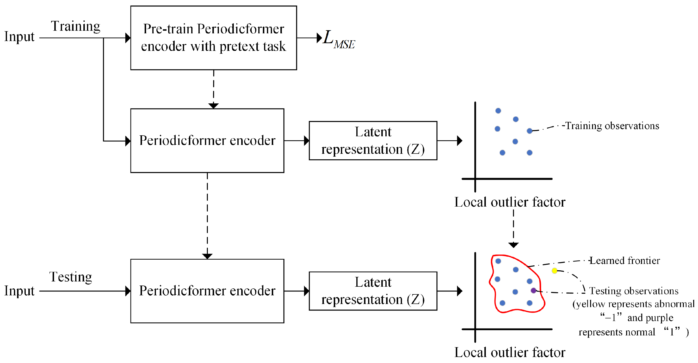
Figure 1 presents the proposed ETD framework, which explicitly consists of two main phases: model training and model testing. The training phase consists of two steps: Step 1: Pre-train the Periodicformer encoder by recovering partially masked input sequences (i.e., unsupervised representation learning). Step 2: Feed the latent representations output by the encoder into local outlier factor (LOF) to learn the anomaly detection boundary. In the testing phase, the input data are fed through the trained Periodicformer encoder and classifier to determine whether testing latent representation is within the trained boundary (1) or not (−1).

3.1. Periodicformer Encoder for Unsupervised Representation Learning

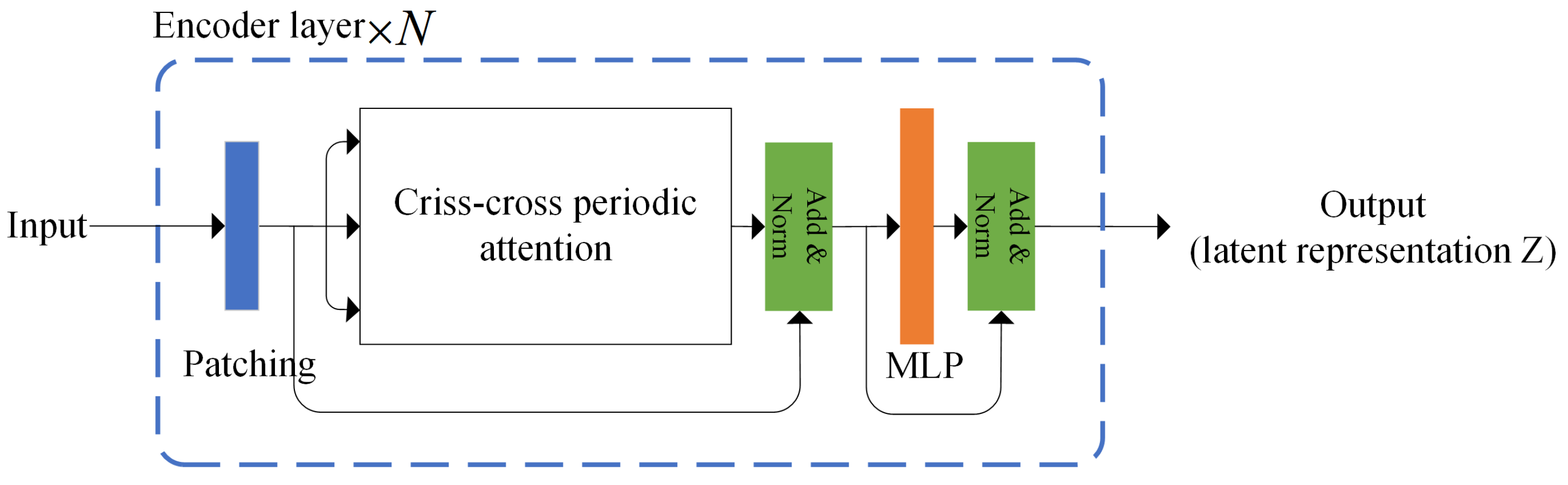
Figure 2 illustrates the overall architecture of the proposed Periodicformer encoder, which is composed of three modules: the patching module, the proposed criss-cross periodic attention module, and the multilayer perceptron (MLP) module (consisting of two linear layers with a GELU activation function).

In layer i, we denote the patch size as $p_i$, the length of the input feature as $L_{i-1}$, and the embedding dimension as d.

3.1.1. Patching Operation

The input feature $F_{i-1}\in {\mathbb{R}}^{L_{i-1}\times d}$ for layer i is first divided into multiple patches. $P=[patc{h}^1,\dots ,patc{h}^{{\displaystyle \frac{L_{i-1}}{p_i}}}]\in {\mathbb{R}}^{{\displaystyle \frac{L_{i-1}}{p_i}}\times (p_i\times d)}$ (${\displaystyle \frac{L_{i-1}}{p_i}}$ is the number of the patches, each patch $\in {\mathbb{R}}^{p_i\times d}$). Then, these patches are flattened and embedded into a new feature map $F_{i-1}^{\prime }=[flatten\left(patc{h}^1\right),\dots ,flatten\left(patc{h}^{{\displaystyle \frac{L_{i-1}}{p_i}}]}\right)]W_P+b_P$.

It is worth noting that we do not use positional encoding here, as our experimental results show that adding positional encoding actually reduces detection performance, which is consistent with the findings in Reference [28].

3.1.2. Criss-Cross Periodic Attention

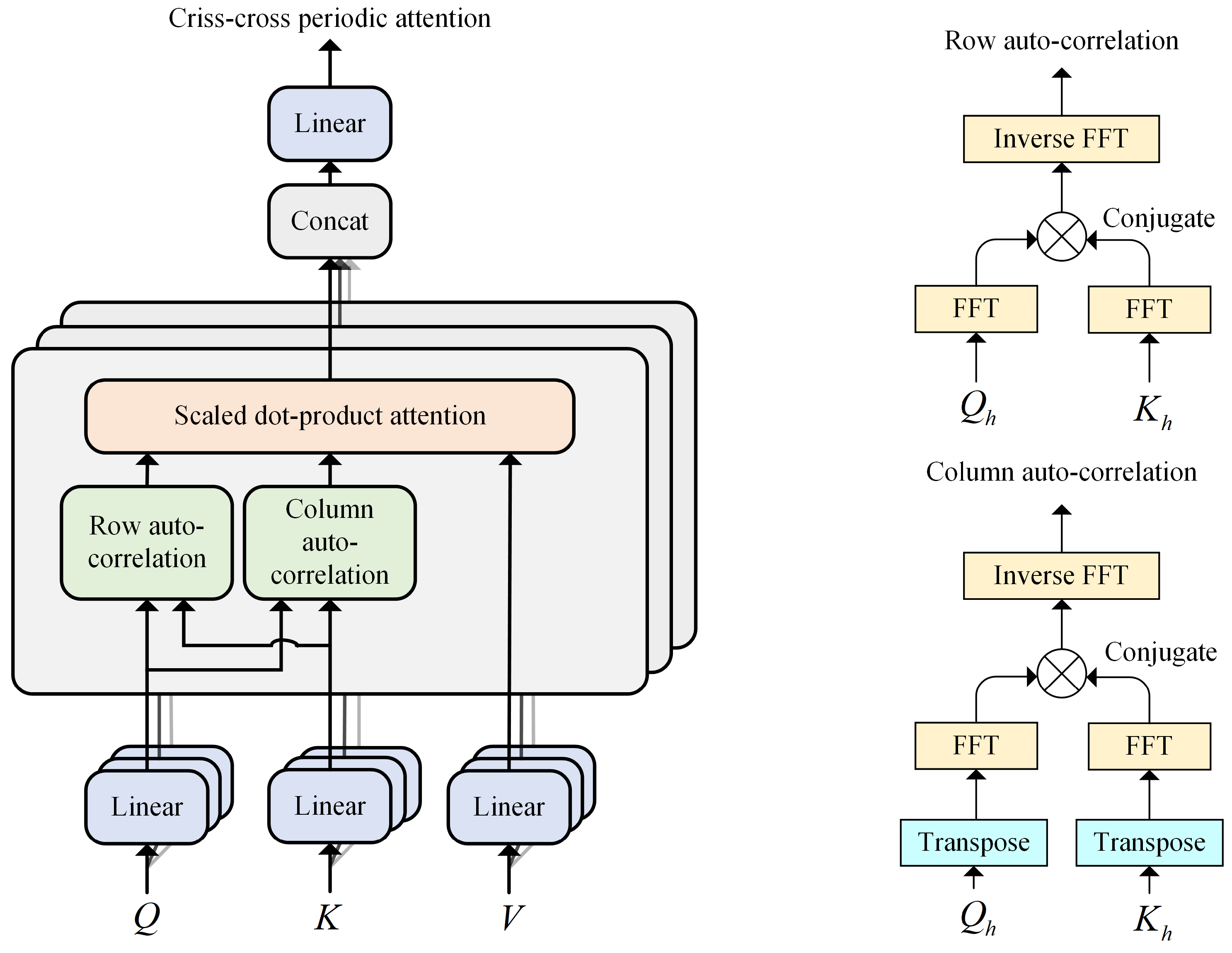
As shown in Figure 3, we propose the criss-cross periodic attention mechanism to mine richer periodic scale characteristics. Row autocorrelation and column autocorrelation explore periodic dependencies by calculating autocorrelation.

• Period-based dependencies: Inspired by the autocorrelation mechanism [29], for an input sequence $X_t$ with length L, we can obtain the autocorrelation $R_{XX}\left(\tau \right)$ by the following Equation (1):

  $$R_{XX}\left(\tau \right)=\underset{L\to \infty }{lim}{\displaystyle \frac{1}{L}}\sum _{t=1}^L{X}_t{X}_{t-\tau },$$

  (1)
  $R_{XX}\left(\tau \right)$ reflects the time-delay similarity between $\left\{X_t\right\}$ and its $\tau$ lag series $\left\{X_{t-\tau }\right\}$. Taking the row autocorrelation in Figure 3 as an example, for single head h and input sequence $F_{i-1}^{\prime }\in {\mathbb{R}}^{L_i\times d}$ where $L_i={\displaystyle \frac{L_{i-1}}{p_i}}$, after the linear projector, we get query $Q_h$, key $K_h$, and value $V_h$. At this point, we consider $Q_h$ as sequences along the row direction, i.e., $Q_h=[ro{w}_1,\dots ,ro{w}_{d_k}]$ where $d_k$ is the embedding dimension of $K_h$, with $K_h$ treated in the same manner. Then, we can obtain the row autocorrelation ${\widehat{R}}_{Row}(Q_h,K_h)$ using the following Equation (2):

  $${\widehat{R}}_{Row}(Q_h,K_h)=[R_{Q_h,K_h}\left(1\right),\dots ,R_{Q_h,K_h}\left(d_k\right)],$$

  (2)

  where $R_{Q_h,K_h}$ is the autocorrelation between $Q_h$ and $K_h$. The calculation of the column autocorrelation is similar to that of row autocorrelation, with the only difference being that $Q_h$ and $K_h$ are treated as sequences along the column direction. The formula for calculating column autocorrelation is provided in Equation (3).

  $${\widehat{R}}_{Column}(Q_h,K_h)=[R_{Q_h^T,K_h^T}\left(1\right),\dots ,R_{Q_h^T,K_h^T}\left(L_i\right)],$$

  (3)

  where $R_{Q_h^T,K_h^T}$ is the autocorrelation between the transpose of $Q_h$ and the transpose of $K_h$;
• Criss-cross periodic attention: To comprehensively capture the different periodic features extracted by row and column autocorrelation, we use the scaled dot product attention, with the product of row and column autocorrelation serving as the new attention weights. For a single head h, the criss-cross periodic attention (CCPA) mechanism is as shown in the following Equation (4):

  $$\mathrm{CCPA}(Q_h,K_h,V_h)=softmax\left({\displaystyle \frac{{\widehat{R}}_{Row}(Q_h,K_h){\widehat{R}}_{Column}^T(Q_h,K_h)}{\sqrt{d_k}}}\right)V_h,$$

  (4)
  For the multi-head version, with H heads, the process is as shown in Equation (5):

  $$\begin{array}{cc}\hfill \mathrm{Multi}-\mathrm{head}(Q,K,V)& =concat(hea{d}_1,\dots ,hea{d}_H)W_o,\hfill \\ \hfill \mathrm{where}hea{d}_i& =\mathrm{Criss}-\mathrm{cross}\mathrm{periodic}\mathrm{attention}(Q_i,K_i,V_i),\hfill \end{array}$$

  (5)
• Efficient computation: The Wigner–Khinchin theorem establishes that the Fourier transform of the autocorrelation function of a signal equals its power spectral density. For the autocorrelation computation (Equation (1)), the given input sequence $X_t$, $R_{XX}\left(\tau \right)$ can be calculated by the discrete Fourier transforms (DFT) as Equation (6):

  $$\begin{array}{cc}\hfill \mathcal{F}\left(X_t\right)& =\sum _{t=1}^L{X}_t{e}^{-2\pi i{\displaystyle \frac{kt}{L}}},\hfill \\ \hfill S_{XX}\left(k\right)& =\mathcal{F}\left(X_t\right){\mathcal{F}}^{*}\left(X_t\right),\hfill \\ \hfill R_{XX}\left(\tau \right)& ={\mathcal{F}}^{-1}\left(S_{XX}\left(k\right)\right)={\displaystyle \frac{1}{L}}\sum _{k=1}^L{S}_{XX}\left(k\right)e^{2\pi i{\displaystyle \frac{k\tau }{L}}},\hfill \end{array}$$

  (6)

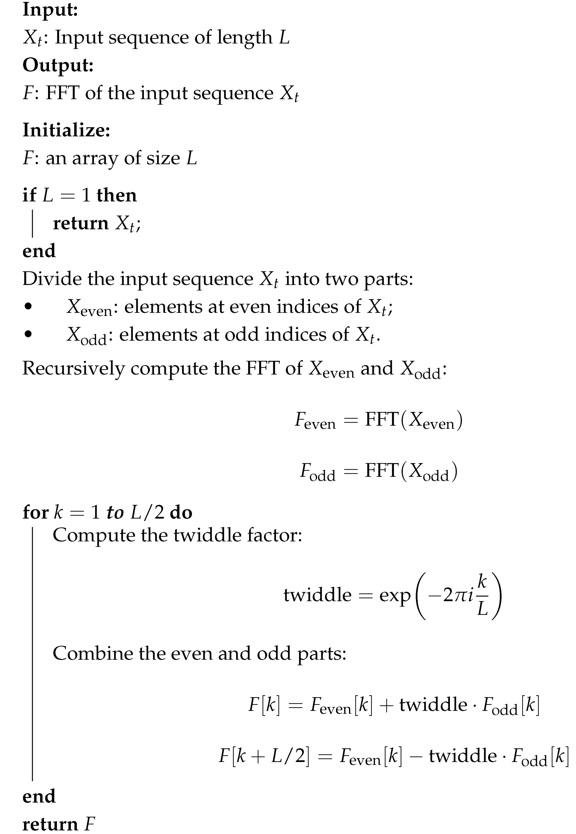
  where $\tau \in \{1,\dots ,L\}$, $\mathcal{F}$ denotes DFT and ${\mathcal{F}}^{-1}$ is its inverse transformation. ∗ denotes the conjugate operation, and $S_{XX}\left(k\right)$ is the power spectral density. In practice, we use fast Fourier transforms (FFT) to reduce the time complexity from $O\left(L^2\right)$ to $O(LlogL)$. The FFT algorithm process can be seen in Algorithm 1.

Algorithm 1: Fast Fourier transform (FFT)

3.1.3. Unsupervised Representation Learning

Electricity consumption data are treated as a univariate time series of length T, expressed as $X=\{x_1,\dots ,x_T\}$. To determine whether the data point $x_t$ at time t is an anomaly, we analyze a contextual window of length L, defined as $w_t=\{x_{t-L+1},\dots ,x_t\}$, instead of focusing solely on a single point. The training set can be represented as $X^{\prime }=\{w_L,\dots ,w_T\}$. For simplicity, windows $w_t$ are omitted when $t<L$ [30].

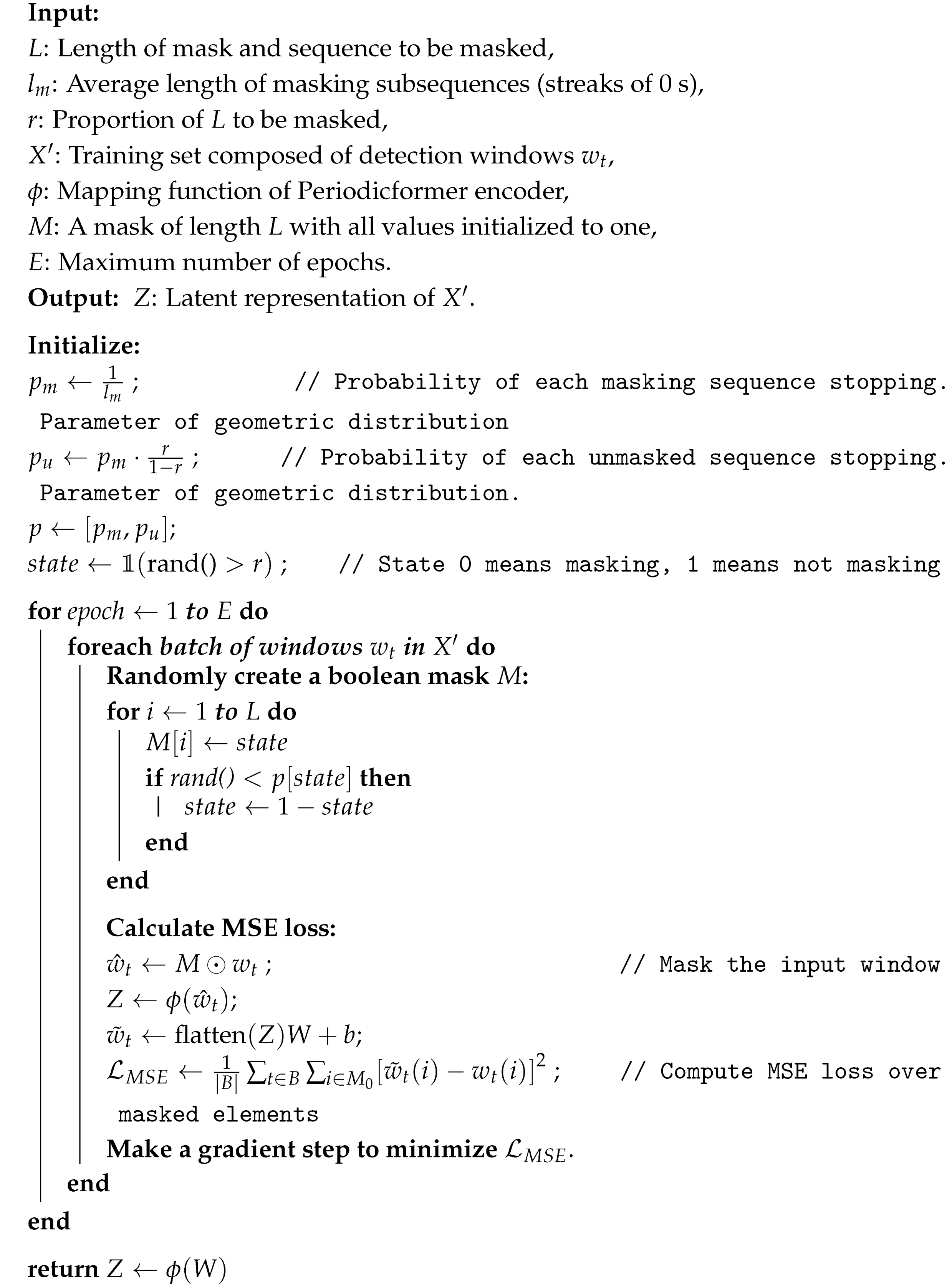
Unsupervised representation learning involves two steps: creating a Boolean mask M and calculating the mean squared error (MSE) loss. The mask M is generated with alternating segments of 0 s and 1 s, where the lengths of the 0 s and 1 s follow geometric distributions with means $l_m$ and $l_u$, respectively. The proportion r determines the ratio of 0 s in the mask, and the length $l_u$ is computed as $l_u={\displaystyle \frac{1-r}{r}}{l}_m$. The masked detection window ${\widehat{w}}_t$ is then passed through the encoder, producing feature representation Z. The output Z is flattened and passed through a linear layer to forecast the masked values, yielding ${\tilde{w}}_t$. The MSE loss is computed by comparing the predicted values ${\tilde{w}}_t\left(i\right)$ to the actual masked values $w_t\left(i\right)$ at the indices in $M_0$, which are the positions where $M\left(i\right)=0$, as Equations (7)–(9).

$${\widehat{w}}_t=M\odot w_t$$

(7)

$${\tilde{w}}_t=flatten\left(Z\right)W+b$$

(8)

$${\mathcal{L}}_{MSE}={\displaystyle \frac{1}{\left|B\right|}}\sum _{t\in B}\sum _{i\in M_0}{\left[{\tilde{w}}_t\left(i\right)-w_t\left(i\right)\right]}^2$$

(9)

where ⊙ is the Hadamard product, B is a batch of training samples, and $\left|B\right|$ represents the batch size. The overall process of unsupervised representation learning is described in detail in Algorithm 2.    

Algorithm 2: Unsupervised representation learning

Note that the objective of the unsupervised representation learning is to learn latent representations Z for subsequent one-class classification-based anomaly detection. In the subsequent anomaly detection process, the linear layer originally used for outputting the masked time series is discarded.

3.2. One-Class Classifier for Anomaly Detection

Once the unsupervised training is completed, the training data are rejected into the trained Periodicformer encoder and the latent representation ($Z=\{z_1,\dots ,z_{|X_{tr}|}\}$) is fed to the local outlier factor (LOF) as input where $|X_{tr}|$ is the number of training data.

LOF is a density-based outlier detection algorithm. The determination of the outlier is judged based on the density between each data point and its neighbor points. The lower the density of the point, the more likely it is to be identified as the outlier. The key definitions for the LOF are as follows:

Definition 1.

k-distance of data point $z_p$. For a given dataset D and any positive integer k, the k-distance of $z_p$, denoted as $k-\mathrm{distance}\left(z_p\right)$, is defined as the distance $d(z_p,z_o)$ between data point $z_p$ and data point $z_o$ in the following conditions:

• For at least k data points $z_{o^{\prime }}\in D\setminus \left\{z_p\right\}$, it holds that $d(z_p,z_{o^{\prime }})\le d(z_p,z_o)$;
• for at most $k-1$ objects $z_{o^{\prime }}\in D\setminus \left\{z_p\right\}$, it holds that $d(z_p,z_{o^{\prime }})<d(z_p,z_o)$.

Definition 2.

k-distance neighborhood of data point $z_p$. Given the k-distance of $z_p$, the k-distance neighborhood of $z_p$ contains every data point $z_q$ whose distance from $z_p$ is not greater than the k-distance, as described in Equation (10).

$$N_{k-distance\left(z_p\right)}\left(z_p\right)=\{z_q\in D\setminus \left\{z_p\right\}|d(z_p,z_q)\le k-distance\left(z_p\right)\}$$

(10)

Definition 3.

Reachability distance of data point $z_p$ with respect to data point $z_o$. Let k be a natural number. The reachability distance of $z_p$ with respect to $z_o$ is defined as Equation (11).

$${reach-dist}_k(z_p,z_o)=max(k-distance\left(z_o\right),d(z_p,z_o))$$

(11)

Definition 4.

Local reachability density of data point $z_p$. The local reachability density of $z_p$ is defined as Equation (12).

$$lr{d}_k\left(z_p\right)=1/{\displaystyle \frac{{\sum }_{z_o\in N_k\left(z_p\right)}{reach-dist}_k(z_p,z_o)}{|N_k\left(z_p\right)|}}$$

(12)

where $N_k\left(z_p\right)$ is the k-distance neighborhood of data point $z_p$.

Definition 5.

Local outlier factor of data point $z_p$. The local outlier factor of $z_p$ is defined as Equation (13).

$$LO{F}_k\left(z_p\right)={\displaystyle \frac{{\sum }_{z_o\in N_k\left(z_p\right)}\frac{lr{d}_k\left(z_o\right)}{lr{d}_k\left(z_p\right)}}{|N_k\left(z_p\right)|}}$$

(13)

The contamination rate hyper-parameter determines the threshold based on the LOF of the training samples. During testing, data points with LOF values greater than the threshold are considered outliers.

4. Results

We have implemented the entire setup using Python 3.8.17. The Periodicformer encoder model and unsupervised representation learning process were developed with PyTorch 2.0.1 and PyTorch-Ignite 0.3.0, while the one-class classifier model and training process were built using scikit-learn. We use the Adam optimizer to train all models with a learning rate of 0.001. We implement all the methods three times, and report the results as the mean. The equipment used in this study includes an Intel i3-12100F CPU, manufactured by Intel Corporation, headquartered in Santa Clara, CA, USA, and an NVIDIA GeForce RTX 2060 12G GPU, produced by NVIDIA Corporation, also located in Santa Clara, CA, USA.

4.1. Dataset

The dataset utilized in this study for experimental evaluation is the publicly available electricity consumption dataset from the Irish CER Smart Metering Project [31]. It includes daily electricity consumption records for approximately 5000 residential and commercial users. Details of Irish dataset are shown in

Table 1. Details of Irish dataset.

Descriptions	Values
Number of smart meters	25,730
Time span	14 July 2009–31 December 2010
Recording interval	30 min

.

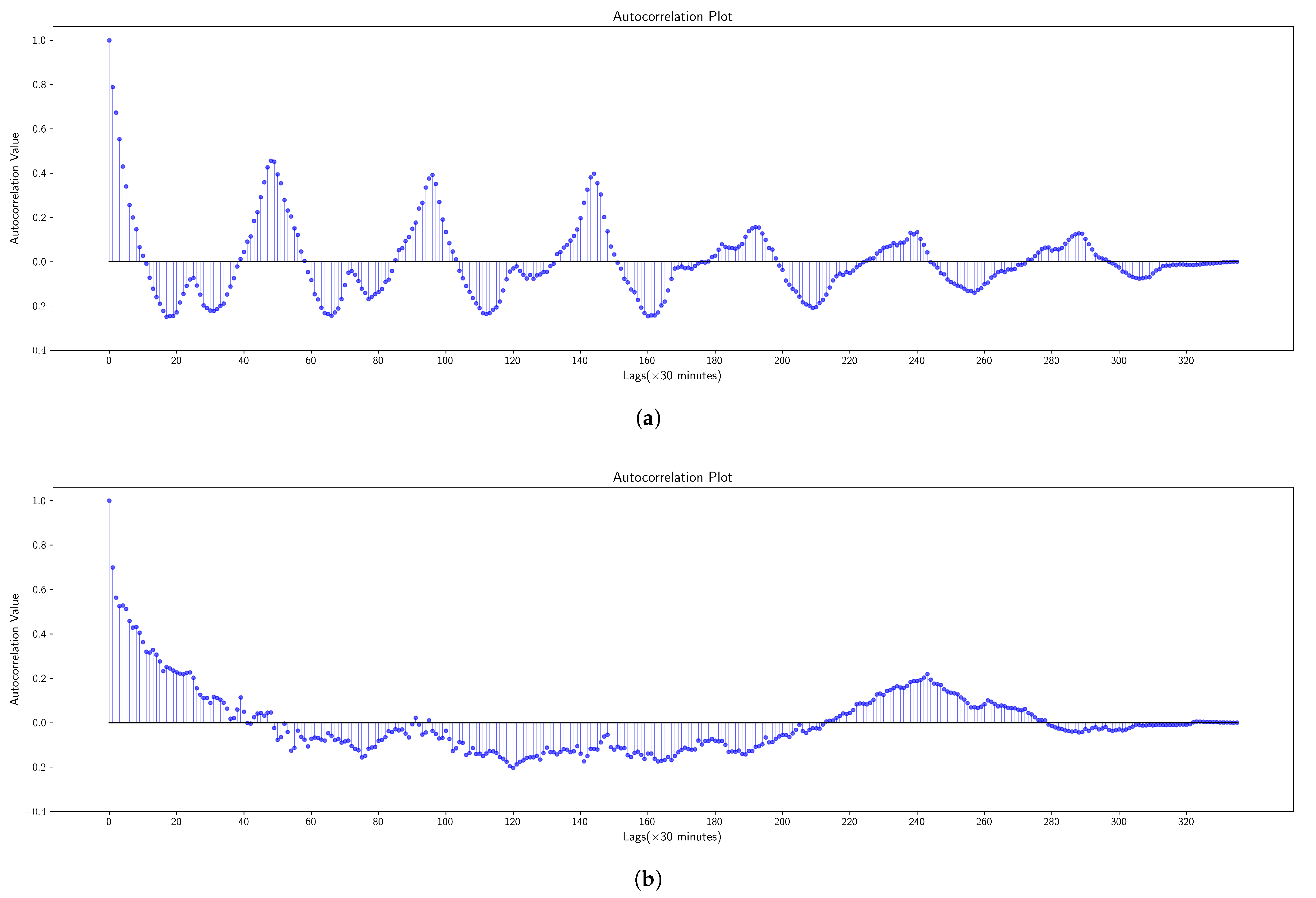
For the experiments, we use data collected over a 365-day period. We exclude users with missing values (NaN), correct erroneous data, and apply min-max normalization to preprocess the dataset [13]. To enhance detection performance, the detection window is set to cover 7 days ($L=336$) instead of a single day. We indeed assume that the distribution of electricity usage data exhibits periodicity within the 7-day detection window for each day. As shown in the Figure 4, we plotted the autocorrelation graphs for both normal and abnormal samples. It is clear that in the autocorrelation graph of the normal sample, the electricity usage data distribution shows periodicity, especially with similar usage patterns between consecutive days. In contrast, the autocorrelation graph of the abnormal sample shows almost no periodicity in the electricity usage data distribution. This provides factual support for our designed PE-DOCC. We believe that for legitimate users, their electricity usage data may exhibit periodicity between days, weeks, and months. However, considering that the time complexity of our designed CCPA is $O(LlogL)$, to save computational costs while still capturing sufficient periodic information within the detection window, we have chosen a 7-day detection window. The electricity consumption data from 5000 residential users is split into training, validation, and test sets in a ratio of 8:1:1. The training set is treated as clean, normal data for model training. In the validation and test sets, 10% of the data is randomly selected and tempered using the attack models described in Section 4.2. The validation set is utilized for hyper-parameter tuning, while the test set is reserved for evaluating the model’s anomaly detection performance.

4.2. Attack Model

False data injection is a type of cyber attack in which manipulated or false information is deliberately introduced into a system to mislead its operations or decision-making processes. It is commonly employed to compromise the integrity of data in power systems, sensor networks, and other critical infrastructures.

In this study, to simulate various electricity theft patterns, six different false data injection attacks are implemented [32,33], as shown in

Table 2. Six types of FDI attacks.

Attack Type	Modification
1	${\tilde{x}}_t={\alpha }_t{x}_t,{\alpha }_t=random(0.2,0.8)$
2	${\tilde{x}}_t=max(x_t-\gamma ,0),\gamma <max\left(X\right)$
3	${\tilde{x}}_t=min(x_t,\gamma ),\gamma <\max \left(X\right)$
4	${\tilde{x}}_t=\left\{\begin{array}{cc}0,\hfill & t_{start}<t<t_{start}+\Delta t\hfill \\ x_t,\hfill & otherwise\hfill \end{array}\right.$
5	${\tilde{x}}_t=\alpha mean\left(X\right),\alpha =random(0.2,0.8)$
6	${\tilde{x}}_t=x_{n-t}$

. $X=\{x_1,x_2,\cdots ,x_{48}\}$ represents the electricity consumption data for a day, and ${\tilde{x}}_t$ denotes the data at time t after being subjected to an attack. $\Delta t=random(0.2,0.8)\times 48$ is the randomly chosen time period throughout a day. $t_{start}=random(0,48-\Delta t)$ is the randomly selected starting times, needing to meet that $t_{start}+\Delta t\le 48$. These attacks are broadly categorized into two types: reduced consumption attacks and load profile shifting attacks [1]. Types 1–4 primarily reduce the electricity consumption recorded by the meter, while Types 5 and 6 shift electricity usage from high-price periods to low-price periods.

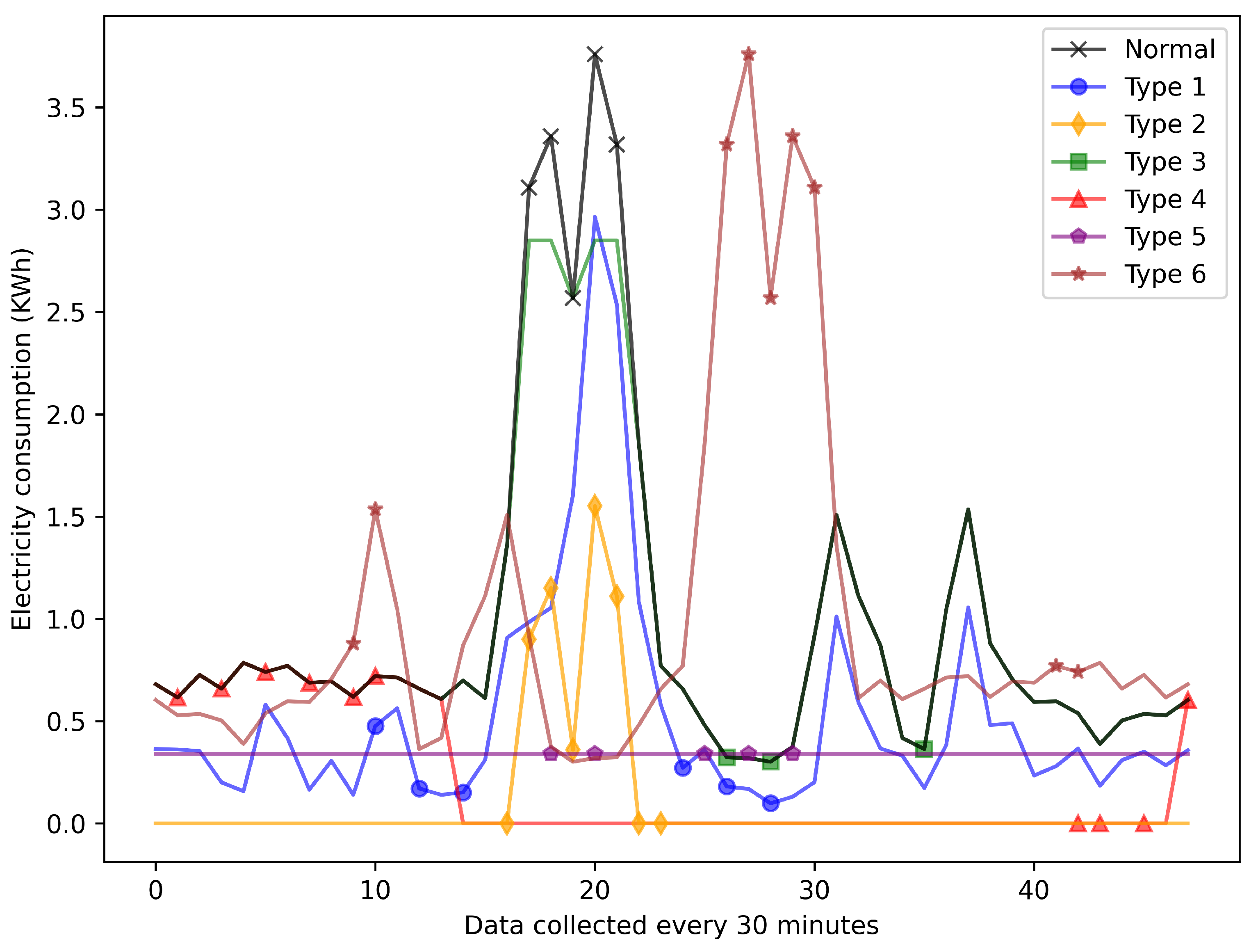
The physical interpretations of these six attacks are as follows: FDI1: Electricity consumption recorded at each time point is scaled down by a randomly selected proportion. FDI2: A constant value is subtracted from the electricity consumption data. FDI3: Electricity consumption values exceeding a preset threshold are capped at the threshold value. FDI4: Consumption data within a randomly selected time interval during the day are replaced with zeros. FDI5: The total daily electricity consumption is evenly distributed across all recording points and reduced by a fixed proportion. FDI6: The entire daily electricity consumption profile is inverted. Additionally, Figure 5 illustrates examples of both normal electricity consumption data and data affected by each of these six attack types.

4.3. Evaluation Metrics

The confusion matrix quantifies all classification outcomes of a model, providing an intuitive representation of classification accuracy. In this paper, electricity theft samples are considered as the positive class, while normal electricity usage samples are treated as the negative class. The definitions of true positive (TP), false positive (FP), false negative (FN), and true negative (TN) are summarized in

Table 3. Confusion matrix of electricity theft detection results.

Samples	Predicted Negative	Predicted Positive
Actually negative	TN	FP
Actually positive	FN	TP

.

Based on the above confusion matrix, we use the F1 score (F1), the area under the receiver operating characteristic (ROC) curve (AUC), recall, and false positive rate (FPR) to evaluate the performance of the proposed electricity theft detection framework.

$Recall$, also known as true positive rate ($TPR$), evaluates a model’s effectiveness in identifying all actual positive instances within a dataset, highlighting its sensitivity to true positives. It is calculated as follows.

$$Recall={\displaystyle \frac{TP}{TP+FN}}$$

(14)

$FPR$ quantifies the rate at which negative samples are misclassified as positive, reflecting the model’s tendency for false alarms. It is computed as follows:

$$FPR={\displaystyle \frac{FP}{FP+TN}}$$

(15)

In anomaly detection, we generally aim for a model that has a low FPR while maintaining a high TPR.

$Precision$ quantifies the accuracy of positive predictions, calculated as follows:

$$precision={\displaystyle \frac{TP}{TP+FP}}$$

(16)

$F1$ captures the trade-off between precision and recall, offering a single metric to evaluate performance, particularly in scenarios with imbalanced data. It is calculated as follows:

$$F1={\displaystyle \frac{2\times precision\times recall}{precision+recall}}$$

(17)

AUC evaluates a model’s capability to differentiate between classes over varying decision thresholds, with larger values reflecting stronger discriminative power.

Model size reflects the storage space occupied by the model file. For devices with limited storage resources (such as smart meters), a smaller model size is important. In this article, model size refers to the size of the trained DNN model. The OC classifier (e.g., OCSVM/iForest/LOF) requires negligible additional storage.

Training time refers to the time required for a model to complete a full training cycle on the training data. For models in electricity theft detection that require frequent updates or retraining, a shorter training time is important. In this article, the training time is the sum of the DNN training time and the OC classifier training time.

Prediction speed reflects how many observations per second the model can process. For scenarios that require rapid response (such as electricity theft detection), a higher prediction speed is necessary.

4.4. Analysis of Model Hyper-Parameters

We applied grid search on the validation set to identify the optimal hyper-parameters. The selection ranges for each parameter and the corresponding best results are presented in

Table 4. Selection of hyper-parameters.

Hyper-Parameter	Range of Values	Optimal Value
k	100, 200, 300	200
contamination rate	0.01, 0.1, 0.2	0.01
distance metric	‘manhattan’, ‘euclidean’	‘euclidean’
d	64, 128	128
H	8, 16	8
N	2, 3, 4	3

.

For the Periodicformer encoder, the hyper-parameters primarily consist of three components: the number of heads H, the encoder embedding dimension d, and the number of layers N. The best results for H, d, and N in this paper are consistent with those in Reference [34]. As for the patch size for each layer $p_i$, this paper empirically concludes that the patch size should initially be larger and then gradually decrease. For LOF, we explore three values for number of neighbors k, and test three different values for the contamination rate parameters to control the expected proportion or number of anomaly points. Additionally, we experiment two different distance metrics. The best combination of parameters was selected based on performance.

4.5. Comparison with Other Methods

In this part, we compare the the proposed method with six one-class classification-based ETD methods. We implement all these methods on the preprocessed data for fair comparison.

• OCSVM [35]: OCSVM is a support vector machine-based algorithm designed for anomaly detection. It distinguishes normal samples from anomalies by maximizing the margin between the data and the origin in the feature space. We set the kernel function and $\nu$ parameters as ’linear’ and 0.2, respectively;
• iForest [36]: iForest is an efficient unsupervised anomaly detection method leveraging random forests. It isolates anomalies by exploiting their tendency to be easier to separate from the majority of the data through random partitioning. We set the contamination, maxFeatures, and nEstim parameters as 0.1, 0.6, and 300, respectively;
• LOF [37]: LOF is a density-based anomaly detection algorithm. It detects outliers by comparing the local density of a sample with the densities of its neighbors, identifying anomalies as points with significantly lower densities. We set the contamination rate as 0.1 while keeping other parameters as default;
• Autoencoder with one-class (OC) classifier [26]: Reference [26] incorporates the concept of autoencoding and OC classification. We implement this method using CNN-AE(1D) as the autoencoder along with three OC classifiers.

Figure 6 shows the confusion matrix of different methods. Based on the confusion matrix, we can calculate recall, FPR, precision, and F1 score using the formulas mentioned above.

Table 5. Performance of different methods.

Model for Unsupervised Representation Learning	OC Classifier	Metrics
		F1	AUC	Recall	FPR	Model Size (bytes)	Training Time (s)	Prediction Speed (obs/s)
-	OCSVM	0.434	0.893	0.816	0.217	-	0.54	50,076.87
	iForest	-	-	-	-		1.29	21,742.70
	LOF	-	-	-	-		0.97	24,930.60
Autoencoder	OCSVM	0.477	0.917	0.890	0.209	$0.17\times {10}^6$	142.31	1761.15
	iForest	0.402	0.840	0.743	0.223		134.90	1881.23
	LOF	0.814	0.952	0.856	0.027		133.89	1831.21
Periodicformer encoder	OCSVM	0.517	0.940	0.918	0.189	$3.11\times {10}^6$	725.39	155.04
	iForest	0.434	0.860	0.752	0.194		717.94	154.39
	LOF	0.833	0.973	0.877	0.025		716.93	151.32

presents the comparison results between our proposed method and six baseline methods, and the following findings can be observed:

• Overall, the combination of the Periodicformer encoder and LOF achieved the best performance, with F1, AUC, recall, and FPR scores of 0.833, 0.973, 0.877, and 0.025, respectively. Compared to the second-best approach, the combination of autoencoder and LOF (F1, AUC, recall, and FPR scores of 0.814, 0.952, 0.856, and 0.027, respectively), it achieved improvements of 2.3%, 1.7%, 2.4%, and 8% in F1, AUC, recall, and FPR, respectively.
• The three approaches that rely solely on the OC classifier exhibit relatively poor anomaly detection performance, with some even failing (defined as AUC or recall values below 0.5). This observation aligns with the findings reported in Reference [26]. This suggests that the one-class classifier fails to effectively capture the distribution of normal samples in the training dataset, making it difficult to distinguish between normal and anomalous samples in the test set. This underscores the importance of designing a robust unsupervised representation learning method to extract meaningful features, aiding the one-class classifier in better modeling the distribution of normal samples and improving anomaly detection performance.
• Comparing the proposed combination of the Periodicformer encoder and OC classifier with the combination of autoencoder and OC classifier, specifically the combination of the Periodicformer encoder and LOF versus autoencoder and LOF, the Periodicformer encoder demonstrates superior suitability for modeling time series data. Additionally, our proposed criss-cross periodic attention further enhances the model’s ability to capture richer periodic features, which helps distinguish normal data from anomalous data. In contrast, the autoencoder relies solely on CNN to capture local features without considering the periodicity of time series data, resulting in poorer performance;
• In the three combinations of the Periodicformer encoder with different OC classifiers, the scheme combined with iForest yields the poorest performance. According to Reference [38], iForest is sensitive only to global outliers and struggles with detecting local outliers. The distribution of power theft behavior data is particularly unfavorable for iForest detection. For instance, when considering an entire year (365 days), power theft typically occurs on specific days or weeks. These anomalies may not be noticeable when viewed in the context of the whole year. However, when compared to adjacent days or weeks, these outliers may become more apparent. This is precisely where iForest’s limitations lie. Regarding the combination with OCSVM, Reference [39] states that OCSVM is sensitive to noise and prone to false positives, which aligns with our experimental findings. Although it achieves a high recall, it also results in a relatively high false positive rate.
• Compared to the other six methods, our proposed PE-DOCC has a larger model size ($3.11\times {10}^6$ bytes, which is approximately 3.11 MB), a longer training time (around 700 s), and a slower prediction speed (around 150 observations per second). However, in our experimental scenario with 5000 users uploading electricity consumption records every 30 min, we can calculate that the minimum acceptable and reasonable prediction speed range is 3–5 observations per second. Our prediction speed far exceeds this range, meeting the requirements for this scenario. Additionally, the model size is only 3.11 MB, which is also applicable for a smart meter. 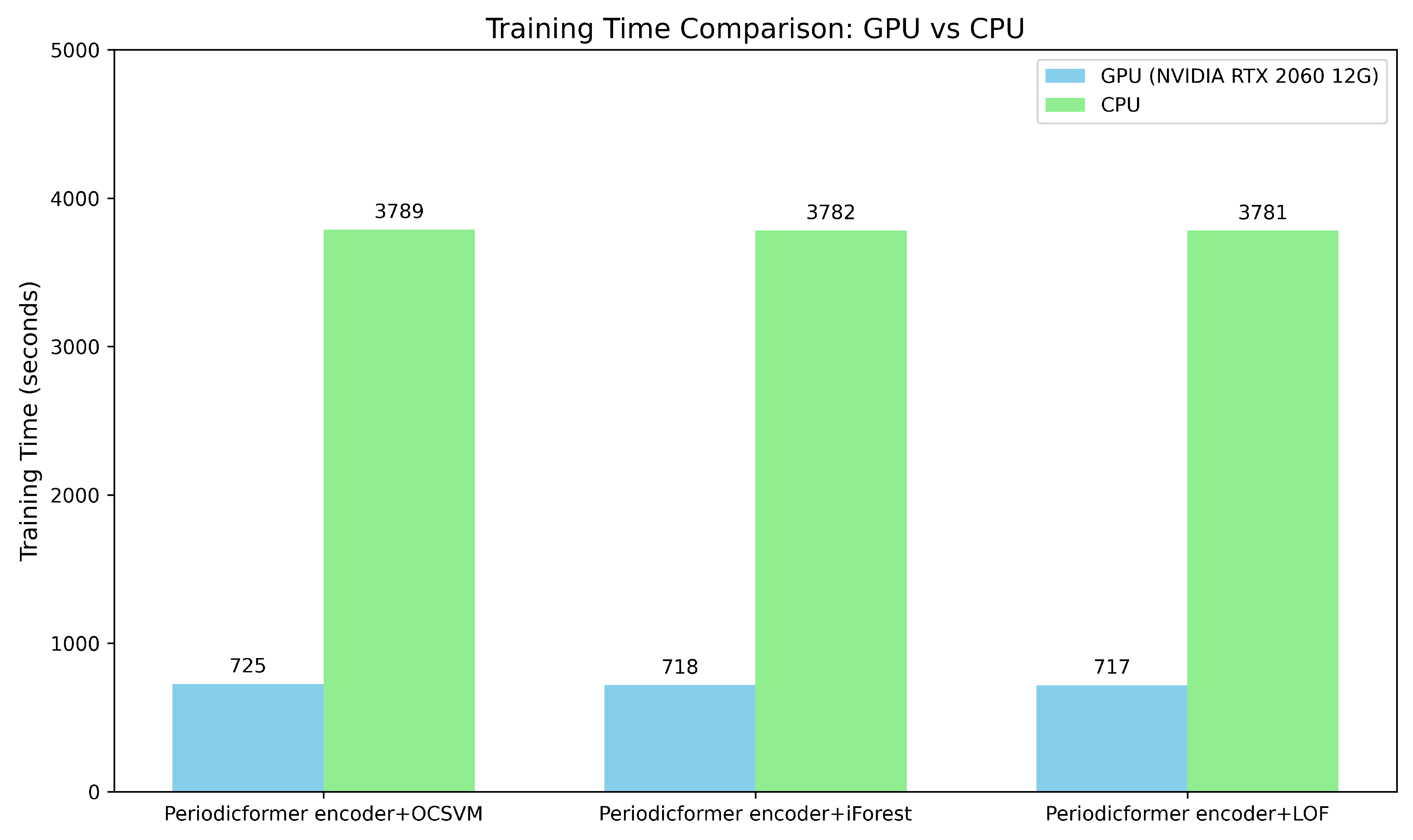Figure 7 compares the training time of the proposed PE-DOCC with GPU acceleration (NVIDIA GeForce RTX 2060 12 G) and without GPU acceleration (CPU). The training time of our proposed PE-DOCC solution on a CPU is approximately 3780 s, which is about one hour. The training for electricity theft detection is typically conducted offline, and our solution follows the same approach; thus, it does not affect the efficiency of real-time detection. If the model requires daily updates, the one-hour training time can be scheduled during off-peak hours (e.g., early morning) without impacting real-time predictions. If the model only needs to be updated weekly or monthly, the one-hour training time is entirely acceptable and will not impose any significant burden on the system.

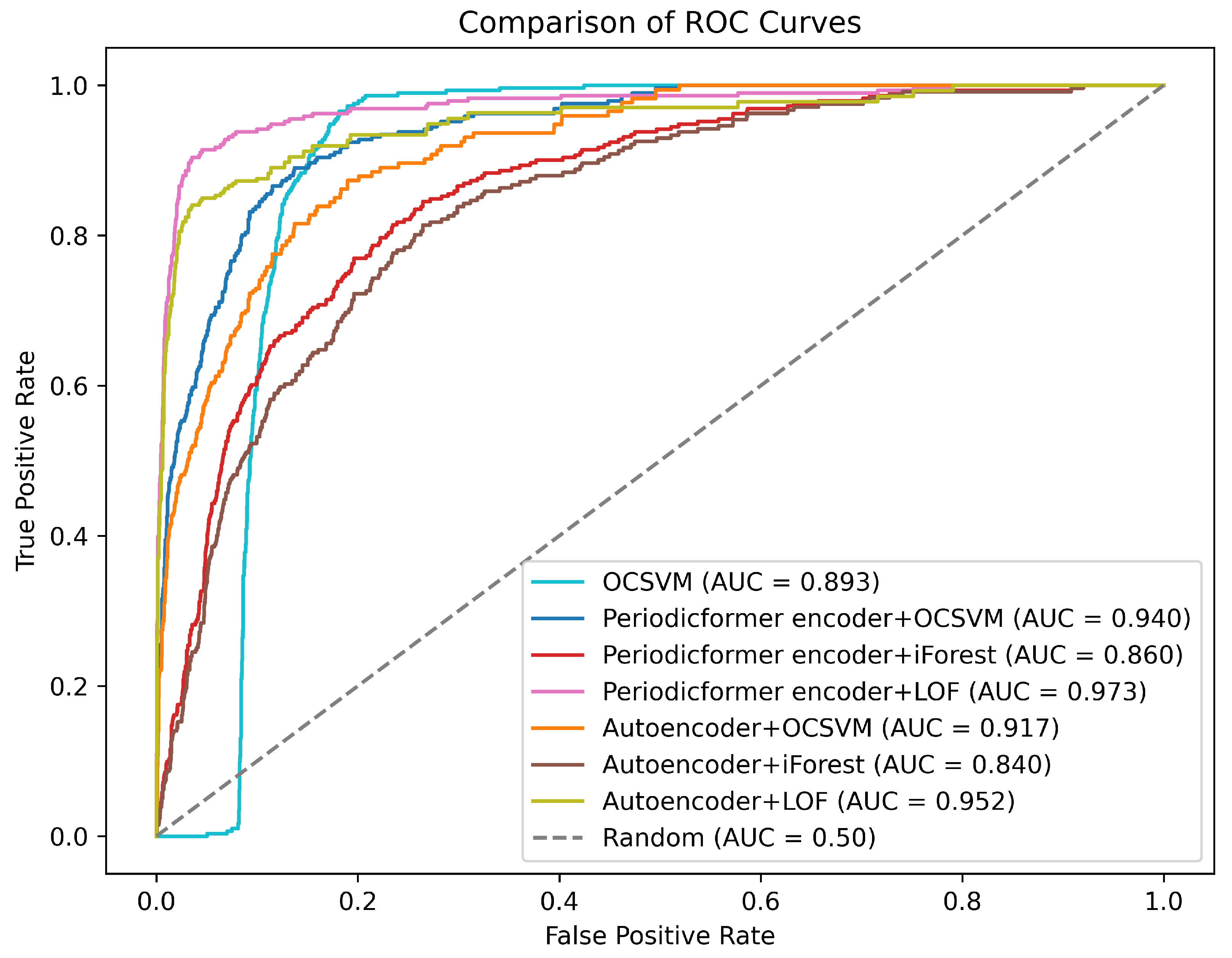
For anomaly detection tasks, our goal is to develop a model that achieves a low false positive rate (FPR) while maintaining a high true positive rate (TPR). To showcase the performance of all the methods in this regard, we have plotted the ROC curve, as shown in Figure 8. The proposed combination of the Periodicformer encoder and LOF achieves the highest TPR at the lowest FPR, and the combination of autoencoder, and iForest yields the poorest performance.

Figure 7. Comparison of training time with and without GPU acceleration.

Figure 7. Comparison of training time with and without GPU acceleration.

Figure 8. ROC curves of the proposed method and other methods and the value of the area under each curve AUC.

Figure 8. ROC curves of the proposed method and other methods and the value of the area under each curve AUC.

4.6. Ablation Analysis

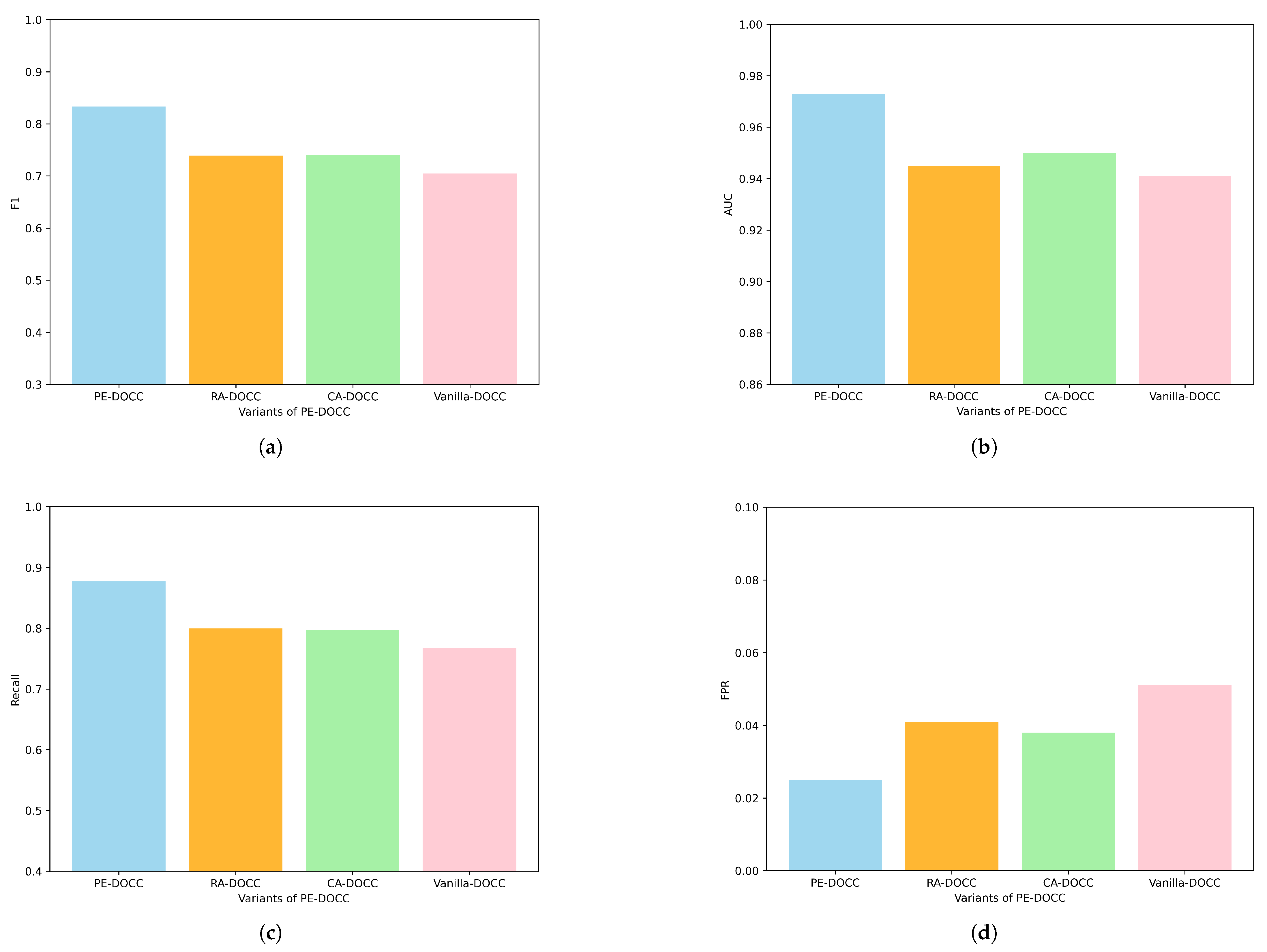
An ablation study is conducted to demonstrate the impact of the main components in the proposed framework on the ETD performance. Specifically, three variants of our proposed method are implemented:

• RA-DOCC: This method uses a combination of a Periodicformer encoder with only row autocorrelation and LOF.
• CA-DOCC: This method uses a combination of a Periodicformer encoder with only column autocorrelation and LOF.
• Vanilla-DOCC: This method uses a combination of a vanilla Transformer encoder [40] and LOF.

Figure 9 shows the results of the ablation experiments, from which the following findings can be drawn:

• RA-DOCC and CA-DOCC produce comparable experimental results, but show notable improvements over Vanilla-DOCC. Specifically, F1, AUC, recall, and FPR improve by approximately 5%, 1%, 4%, and 34%, respectively. This suggests that row autocorrelation and column autocorrelation are all effective in capturing periodic features, which help the model distinguish anomalous samples.
• Our proposed criss-cross periodic attention effectively integrates multiple periodic features. Compared to the vanilla Transformer encoder, F1, AUC, recall, and FPR have improved by 15.3%, 3.2%, 12.5%, and 104%, respectively.

5. Discussion and Conclusions

This paper proposes a novel periodicity-enhanced deep one-class classification framework for electricity theft detection, named PE-DOCC. Overall, the training samples first undergo unsupervised representation learning (i.e., pre-train the Periodicformer encoder). Then, the training samples are passed through the pre-trained encoder to obtain latent representations, which are finally fed into a one-class classifier. During testing, the trained Periodicformer encoder and classifier are used to determine whether the testing latent representation falls within the trained boundary. To enhance the model’s ability to capture periodic features and improve its capacity to distinguish anomalous samples from normal ones, this paper introduces a criss-cross periodic attention mechanism that comprehensively considers both horizontal and vertical periodic features. Experiments are conducted on a real-world electricity consumption dataset, and the results show that the proposed ETD framework can effectively detect anomalous electricity behaviors and outperforms state-of-the-art ETD methods. In future work, we will explore how to use graph neural networks (GNN) to uncover the relationships between different variables in multivariate datasets to further improve model performance.