Torque/Speed Equilibrium Point Monitoring of an Aircraft Hybrid Electric Propulsion System Through Accelerometric Signal Processing

Abstract

The present work proposes a new torque/speed equilibrium point monitoring technique for an aircraft Hybrid Electric Propulsion System (HEPS) through an accelerometric-signal-based approach. Sampled signals were processed using statistical indexes, filtering, and a feature reduction and selection algorithm to train a classification Feedforward Neural Network. A supervised Machine Learning model was developed to classify the HEPS operating modes characterized by an Internal Combustion Engine as a single propulsor or by combining the latter with an Electric Machine used as a motor or a generator. The abnormal changes in the torque/speed equilibrium point were detected by the monitoring index built by computing the Root Mean Square on the value identified by the classifier. The procedure was validated through experimental tests that demonstrated its validity.

1. Introduction

Monitoring is a non-destructive process of system operational condition observation and evaluation to detect any deviations from expected performance. This can involve the use of various sensors and real-time data acquisition systems. In a mechanical system, vibrations are among the most closely monitored variables, and many techniques are available for their monitoring. These techniques analyze signals in the time domain, frequency domain, and time–frequency domain, and they include Machine Learning (ML) methods, Auto-Regressive (AR) models, and hybrid or innovative techniques [1,2,3,4].

One of the most common techniques in the time domain is based on statistical indexes. Bianchini et al. [5] monitored the vibrations of different kinds of submerged pumps, identifying a dependence between vibration and pump power. They summarized this behavior through an experimental equation: the monitoring activity enabled a warning and alarm threshold identification by calculating the Root Mean Square (RMS) value. The lubricant amount monitoring of a gearbox through statistical indexes was reported in [6,7]. McFadden et al. [8] demonstrated how the vibrational signal Time-Synchronous Average (TSA) and combined envelope use can identify bearing damage. Two logarithmic indicators were developed from the vibrational signal TSA extraction to monitor the wear state of a pair of gears [9].

In the frequency domain, De Azevedo et al. [10] studied bearing monitoring by applying the Discrete Fourier Transform (DFT) to sample signals from wind turbines, while Ni et al. [11] proposed a new spectrogram called a Fault Energy of Correntropy diagram that can detect bearing fault frequencies with high precision. This new technique was validated both through simulations and experimental tests. A DFT-based method to monitor a gear transmission was proposed in [12].

In the time–frequency domain, Bartelmus et al. [13] used techniques that transform signals from the time domain to the time–frequency domain, such as the Short-Time Fourier Transform (STFT) and the Wigner–Ville distribution to identify variations in vibrational behavior between a healthy and a damaged planetary gear under different loading conditions. A STFT method to identify gear whine noise using microphones was reported in [14]. Romagnuolo et al. [15] defined an index to detect the cavitation phenomenon in a spoo valve.

Research efforts have been strongly focused on the ML field. Casoli et al. [16] presented a supervised ML classification model comparison, finding that the best model for monitoring an axial piston pump health was the Decision Tree (DT) model. The analysis involved calculating a few features on a raw signal, the signal in the angular domain, and its DFT, which were carefully selected after Principal Component Analysis (PCA). Saxena et al. [17] developed an Artificial Neural Network (ANN) classifier to identify bearing defect types with input features derived from vibrational signals following careful selection through a Genetic Algorithm. An interesting development was a DT model for automotive transmission health monitoring [18]. The authors derived features from vibrational signals in both the time and frequency domains, noting that the best model was the tree trained solely with features from the time domain. Wang et al. [19,20] proposed a Neuro-Fuzzy logic algorithm for the health monitoring of different gear types. Zhang et al. [21] developed new indicators derived from vibrational signal spectral analysis used to train supervised ML classification models.

An Adaptive AR model was proposed in [22] using vibrational signals previously filtered with an Adaptive Kalman Filter (KF) that showed more reliable results compared with other filtering techniques such as TSA. Shao et al. [23] proposed a time-varying AR model with the help of an Extended KF based on residual signals from a gear mesh under healthy conditions for the online monitoring of gearbox vibrations. The model order selection was carried out through hypothesis testing: the developed model was then experimentally tested, showing better results in detecting incipient faults in a gearbox compared with classical analysis techniques but also showing a higher number of false alarms. Siano et al. [24] developed a Non-Linear AR model based on an ANN to simulate pump behavior for monitoring cavitation phenomena: the model outputs were analyzed in both the time and frequency domains, demonstrating reliable results.

Among the most innovative techniques, Feng et al. [25] reviewed works aimed at monitoring gear wear through vibrational analysis, identifying that current highly regarded techniques significantly focus on the development of digital twins. Innovative methodologies based on ML models were reported in [26,27]. Li et al. [28] developed a new technique, Supervised Order Tracking Bounded Component Analysis, demonstrating excellent results in detecting gear cracks in simulations. Feng et al. [29] proposed a new technique combining dynamic models, tribological models, and both simulated and real signals to monitor the surface wear condition of contacting gears. Other techniques involve combining vibrational and acoustic signals [30,31,32] or vibrational and current signals [33,34]. Niola et al. [35] proposed a sensor fusion approach to detect faults in an Internal Combustion Engine (ICE). Zhang et al. [36] proposed a new method for classification problems. Other techniques can be used to monitor mechanical systems [37,38,39,40].

Hybrid Electric Propulsion Systems (HEPS) for aircraft applications are a rapidly developing field, with a lot of studies focusing on energy efficiency [41,42,43] and emission reduction [44,45,46]. The monitoring and diagnostics of HEPS is of fundamental importance. There have been several studies in the literature that address the monitoring of aircraft propulsion systems, but none have focused on accelerometric signals as input data to evaluate their performance. Fentaye et al. [47] developed a Convolutional Neural Network based approach to classify faults in an aircraft engine (AE). Krajček et al. [48] proposed an overview on AE performance monitoring to estimate aircraft parameters. Antoni et al. [49] analyzed the bearing diagnostics of an AE during in transitory conditions using accelerometric signals. Herzog et al. [50] proposed a real-time model-based monitoring technique for the early fault diagnosis of an AE. Adaptive algorithms for AE performance monitoring were proposed in [51,52]. An automatic method for fault detection in satellites and spacecraft systems was presented in [53].

In this paper, a novel technique to monitor the torque/speed equilibrium point of an aircraft HEPS through accelerometric signals combined with a classification Feedforward Neural Network (FNN) is presented. The FNN was trained using the inputs obtained by the processed accelerometric signals acquired from an accelerometer mounted on the load-bearing structure of a HEPS. The FNN output was the HEPS’ operating mode; the ICE completely balanced the propeller resistance torque, the Hybrid Motor and Hybrid Generator modes in which the Electric Machine (EM) operated as a motor and as a generator, respectively. The classification results were used to realize a logical vector. From this vector, an RMS value was calculated. The experimental results demonstrated the index’s capability to monitor the equilibrium point of a HEPS. The focus of this research was training an FNN to accurately classify the three operating modes of a HEPS within torque curve slope variation limits attributed to changes in air properties. If the classification results are incorrect, this implies that the torque/speed equilibrium point falls outside the set limits, and this can be detected using a statistical index calculated based on classification results.

The paper is structured as follows: in Section 2, the HEPS and the tests are described; in Section 3, the workflow is reported; in Section 4, the FNN model and the RMS are briefly explained; and in Section 5, the results are discussed.

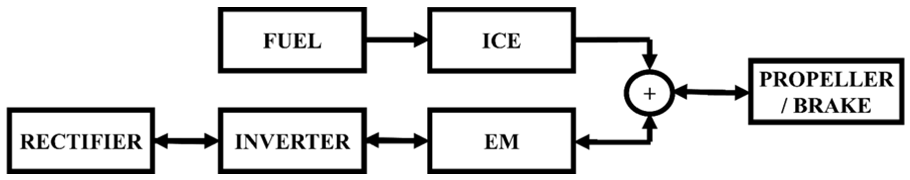
2. HEPS Architecture and Testing Protocol

The proposed HEPS architecture is a parallel type (Figure 1) for aerospace applications consisting of an ICE type CMD 22 and an EM (Electric Machine) type EMRAX 268 Low Voltage (EMRAX, Kamnik, Slovenia), paired with a DC/AC Inverter type GVI-H650 (Parker, Mayfield Heights, Ohio, USA) and a Rectifier type ITECH 500-90 (ITECH, Sassuolo, Italy). Finally, the propeller torque was simulated using a brake type SCHENCK 260 (SCHENCK, Darmstadt, Germany) managed by an APICom MP2030 (APICom, Cento, Italy) bench control system.

The useful drive torque transferred to the propeller $P_{prop}$ is given by the sum of ICE torque $P_{ICE}$ and the EM torque $P_{EM}$:

$$P_{prop}=P_{ICE}+P_{EM}$$

(1)

where the torque $P_{EM}$ is positive if the Electric Machine acts as a motor and thus adds useful axle torque or negative if it subtracts a portion of useful axle torque to generate the electrical energy needed to recharge the batteries. During take-off or climb, the EM operates as a motor, while during descent or landing, the EM functions as a generator. During flight phases such as descent and landing, when low torque is required from the propeller as the aircraft is in the glide phase, the excess torque available from the ICE heat engine could be used to generate electric power and recharge the battery via the generator mode of the EM machine [54,55]. The hybrid configuration in Figure 1 is a parallel type, and the mechanical coupling between the ICE and EM engines is achieved through one-way bearing interposition. This device allows the two engines to be coupled in the propeller positive rotation direction, thereby summing the ICE and EM torques in the hybrid operating mode. More details on the entire experimental setup are provided in [56].

Tests were conducted in the following configurations:

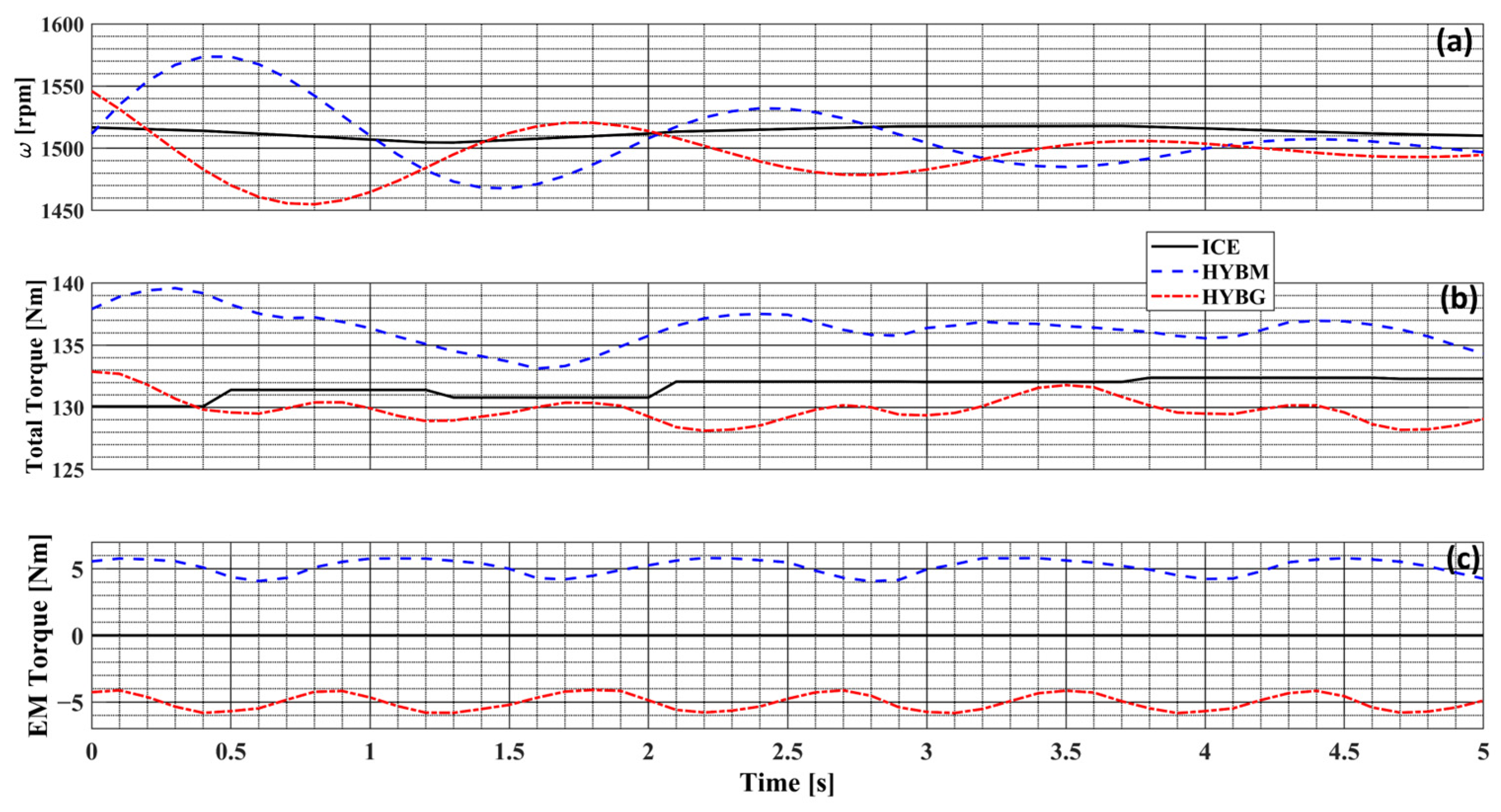
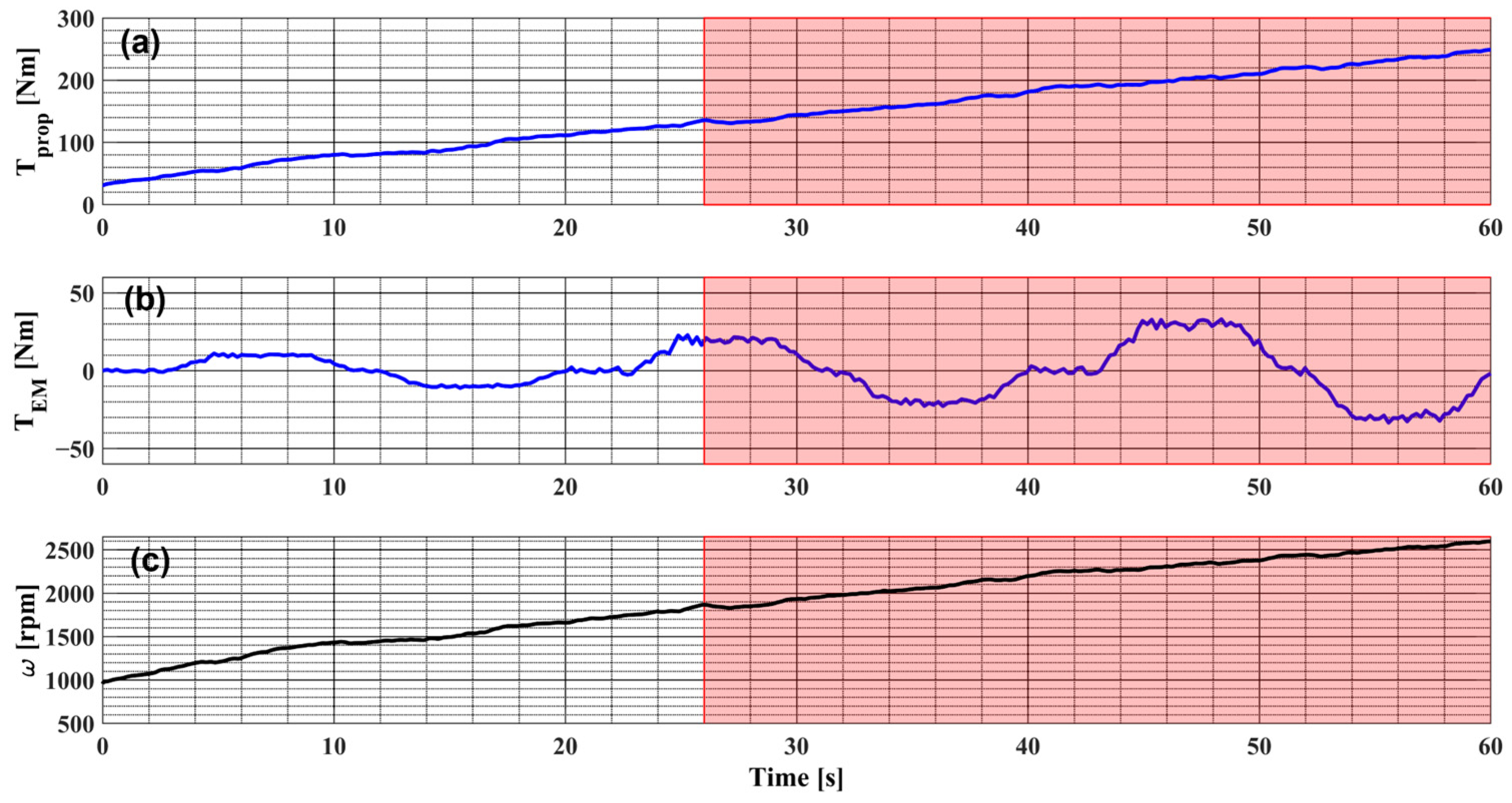
• ICE: only the ICE contributes to balancing the propeller resistance torque ($P_{EM}=0$ and $P_{ICE}=P_{prop}$);
• HYBM: the EM operates as a motor, contributing to balancing the propeller resistance torque ($P_{EM}>0$ and $P_{ICE}=P_{prop}-P_{EM}$);
• HYBG: the EM operates as a generator to recharge the batteries, and the ICE must balance both the propeller and the EM torque ($P_{EM}<0$ e $P_{ICE}=P_{prop}+P_{EM}$)

The tests were performed by alternating the three different HEPS operating modes, ensuring that the equilibrium point was located inside the ±5% limits of propeller torque. Further tests were carried out: the equilibrium point was located outside the limits. These tests were conducted to validate the proposed monitoring technique. Because the HEPS was designed for aircraft that do not fly at considerable altitudes, it is possible to assume that the resistance torque curve is always inside the ±5% limits of the propeller torque curve. For this reason, any deviation of the equilibrium point from the limits is attributed to a change in air properties [57]. During the tests, it was possible to change the equilibrium point because the propeller was simulated by the brake. Figure 2 shows the propeller torque curve and its ±5% limits.

The propeller angular speed was set between 1000 rpm and 2500 rpm, while the total torque was set between 50 and 300 Nm, and the EM torque ranged from −60 to +60 Nm. Vibrational signals were sampled using a triaxial accelerometer, Brüel and Kjaer 4321 type [56], at a frequency of 1 kHz, while the angular speed at the brake and the torques (of the ICE, EM, and brake) were recorded at a frequency of 10 Hz. The choice of this sampling frequency was due to the future goal of testing the proposed algorithm in real time.

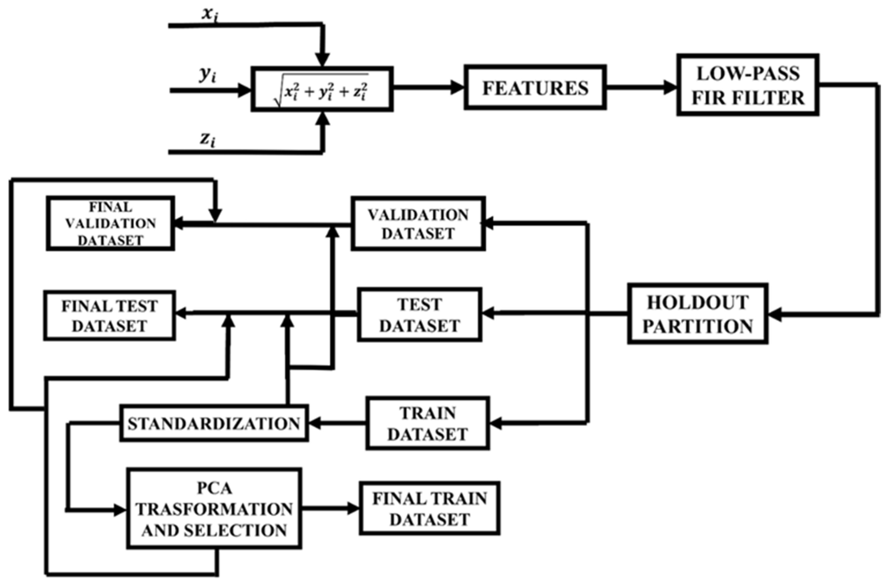
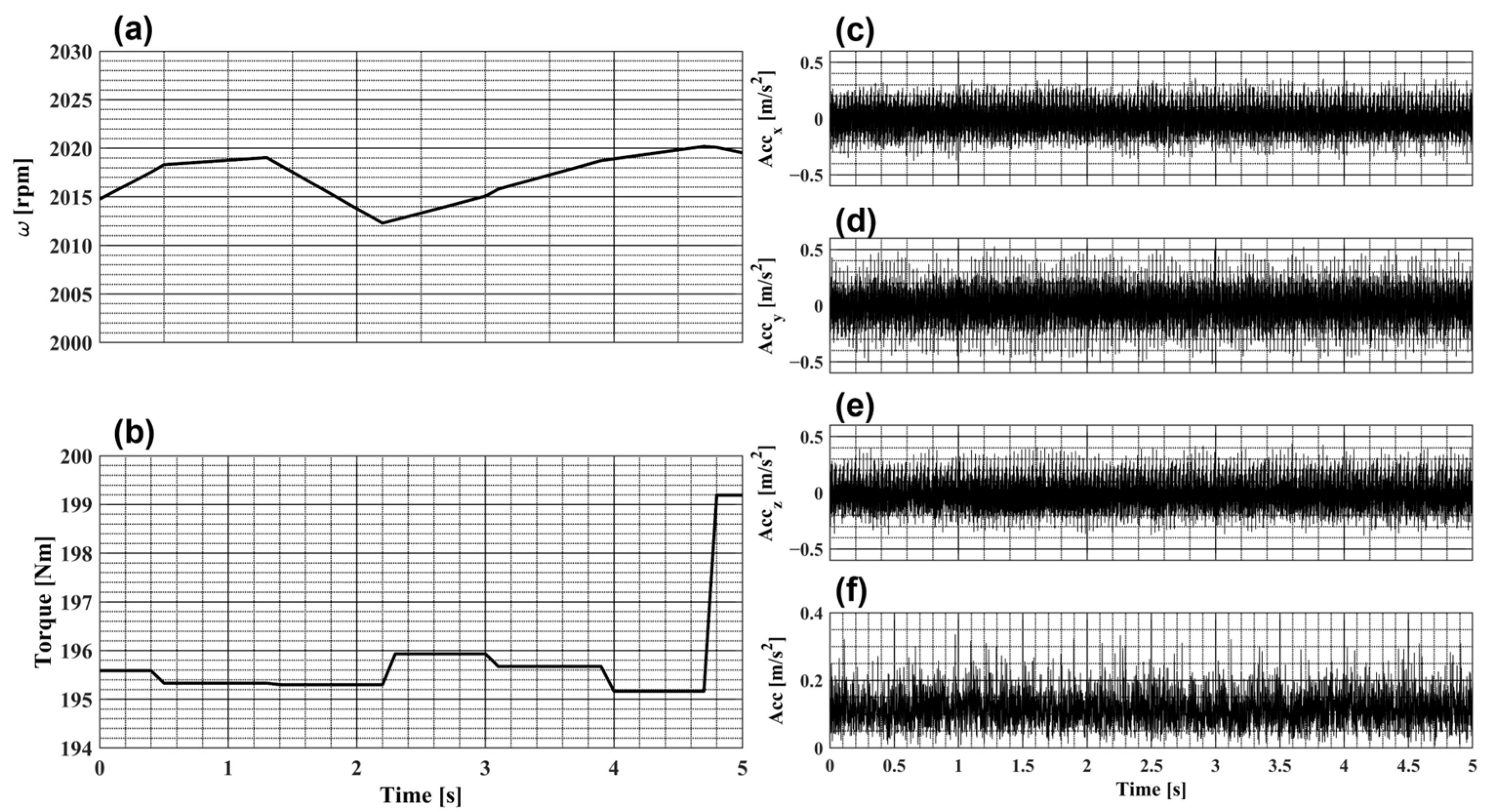
3. Vibration-Based Monitoring Technique: Development Steps

A signal processing workflow was developed to improve the monitoring technique.

To capture the full system vibrational behavior, the magnitude of the 3D space vector was computed by combining the signal components along the three Cartesian axes, and several time-features (statistical indexes) were calculated on the previously mentioned signal. The calculated statistical indexes were mean, median, standard deviation, variance, asymmetry, kurtosis, RMS, crest factor, quadratic oscillation index, harmonic mean, range, amplitude between consecutive points, average between consecutive points, shape factor, impulse factor, clarity factor, vibration index, Pearson correlation index, mode, absolute deviation from mean, absolute deviation from median, and synchrony index. These indexes can describe and synthesize a HEPS’ vibrational behavior.

The HEPS’ vibrational behavior was similar in the three operating modes considering a case in which the torque delivered or absorbed by the EM was close to zero. The features were filtered using a lowpass Finite Impulse Response (FIR) filter to reduce the noise [58]. The indexes were divided into three datasets (training, validation, and testing dataset) using the Holdout method [59]. The mean and the standard deviation were calculated only on the training set for data standardization. The final datasets used as input for the network were reduced with the PCA technique [60,61]. The accuracy of the ML prediction was improved by employing the FIR filter and the PCA. To prevent the unbalance of the model towards a single class, the appearance probability of each class was set equal for all before training the model. The workflow process is summarized in Figure 3.

A Feedforward Neural Network (FNN) [62,63] was developed to predict the HEPS’ operating mode. To minimize the model loss function, the best hyperparameter combination was selected using Bayesian Optimization performed by the Expected Improvement (EI) function [64,65] as the method to model the objective function through a Gaussian Process (GP). Finally, the model accuracy was evaluated.

The workflow process for the FNN training, optimization, and testing phases is shown in Figure 4.

The vibrational signals sampled under operating conditions outside the limits of Figure 2 were processed similarly to the validation and test datasets. This dataset was only used for tests and not to train the FNN: the ML model was only trained and optimized on the dataset obtained from the acquisition in the ±5% limits of the propeller torque curve.

After assigning a 0 value for incorrect model prediction and a 1 value for correct classification, a logical vector was obtained. For every second, an RMS value [66] was calculated to monitor the equilibrium point position in the angular speed–torque plane: if the RMS tended to 1, then the equilibrium point was inside the ±5% limits of the propeller torque curve, while if the RMS decreased and tended to 0, then the equilibrium point was outside the limits. This assumption was validated in experimental tests.

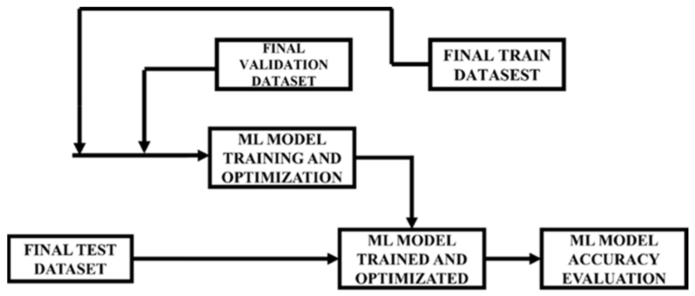
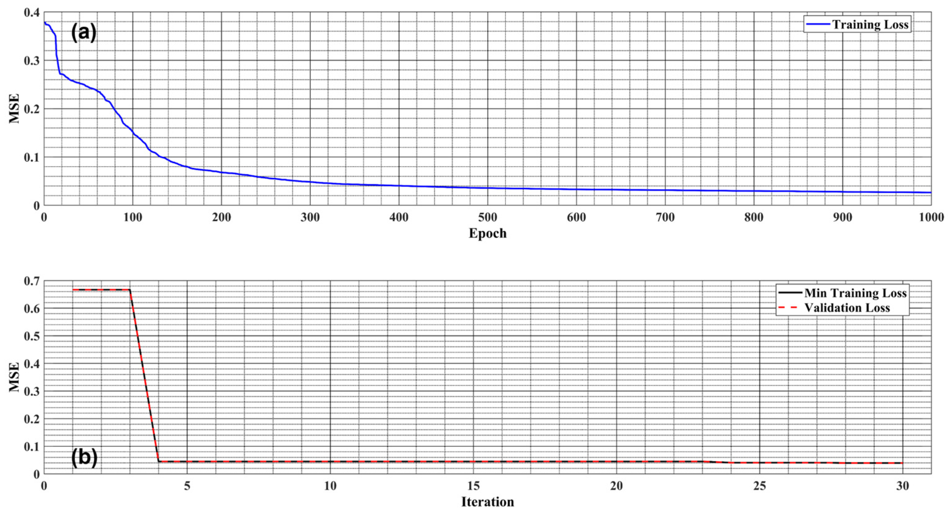
4. Feedforward Neural Network and RMS

An FNN is a supervised ANN where the information flows in a single direction from the input to the output nodes through hidden nodes [62,63]. It is composed of the following:

• An input layer with a number of neurons equal to the number of inputs;
• An output layer with a number of neurons equal to the number of outputs;
• A few hidden layers and corresponding nodes defined through a hyperparameter optimization process.

Each node in every layer of the network is connected to all nodes in the previous and subsequent layers. Considering an FNN with a single hidden layer, the output $z_j$ of $j$-th neuron is modelled as follows:

$$z_j=\sum _{i=1}^n{w}_{ij}{u}_i+b_j$$

(2)

where $w_{ij}$ is the weight assigned to the input $u_i$ in the $j$-th neuron and $b_j$ is the bias associated with the $j$-th neuron. Applying the activation function (also subject to optimization) to the output of the next $j$-th neuron results in the following:

$$y=\sum _{j=1}^n{W}_j{a}_j+B$$

(3)

where $y$ is the output, $W_j$ is the weight of the input $a_j$ of output layer, and $B$ is the bias.

During the network supervised training phase using backpropagation for gradient descent, the FNN adjusts weights and biases based on the assigned input and output variables. This process is repeated over a few epochs or until the loss function reaches a predefined threshold: the goal is to minimize a loss function that measures the difference between the model predictions and the desired values. To achieve these results, it is necessary to iteratively update the model weights to reduce the loss. To optimize the loss function and iteratively update the model weights, the Quasi-Newton BFGS method [67] is applied: its advantage lies in its ability to quickly converge to the global minimum of the loss function, reducing the number of iterations required for convergence.

Among the various activation functions available are ReLU (Rectified Linear Unit), hyperbolic tangent, and SoftMax. The first of these, ReLU, was chosen for the input layer:

$$ReLU\left(x\right)=\left\{\begin{array}{c}x, x>0\\ 0, x\le 0\end{array}\right.$$

(4)

The hyperbolic tangent function was applied as the activation function for the hidden layers:

$$\mathit{Tanh}\left(x\right)={\displaystyle \frac{\mathit{sinh}\left(x\right)}{\mathit{cosh}\left(x\right)}}$$

(5)

For the final layer, the SoftMax activation function, ideal for multi-class classification problems, was used:

$$Softmax \left(x_i\right)={\displaystyle \frac{e^{x_i}}{\sum _j{e}^{x_j}}}$$

(6)

The hyperparameters of an ML model are not learned during the training phase because the objective function is not differentiable with respect to them. To set the best model hyperparameters, it is necessary to use an optimization process such as Bayesian Optimization [64,65], which is a method used to optimize for a higher coast global function when the function is not in closed form. Assuming only observations of unknown function $f\left(·\right)$ are known,

$$y=f\left(x\right)+\epsilon$$

(7)

where $\epsilon$ is the gaussian noise. The Bayesian Optimization process can be expressed below:

$$x^{\ast }=\arg \underset{x}{\max }f\left(x\right)$$

(8)

Using sequential optimization, only $x_t$ at instant $t$ is selected and the objective function $f\left(·\right)$ is modelled as a Gaussina Process.

In the last part of this research, the RMS [66] statistical index was calculated. It is defined as follows:

$$RMS=\sqrt{{\displaystyle \frac{1}{n}} \sum _{i=1}^n{x_i}^2}$$

(9)

where $x_i$ is the $i$-th component of signal $x$ and $n$ is the signal length.

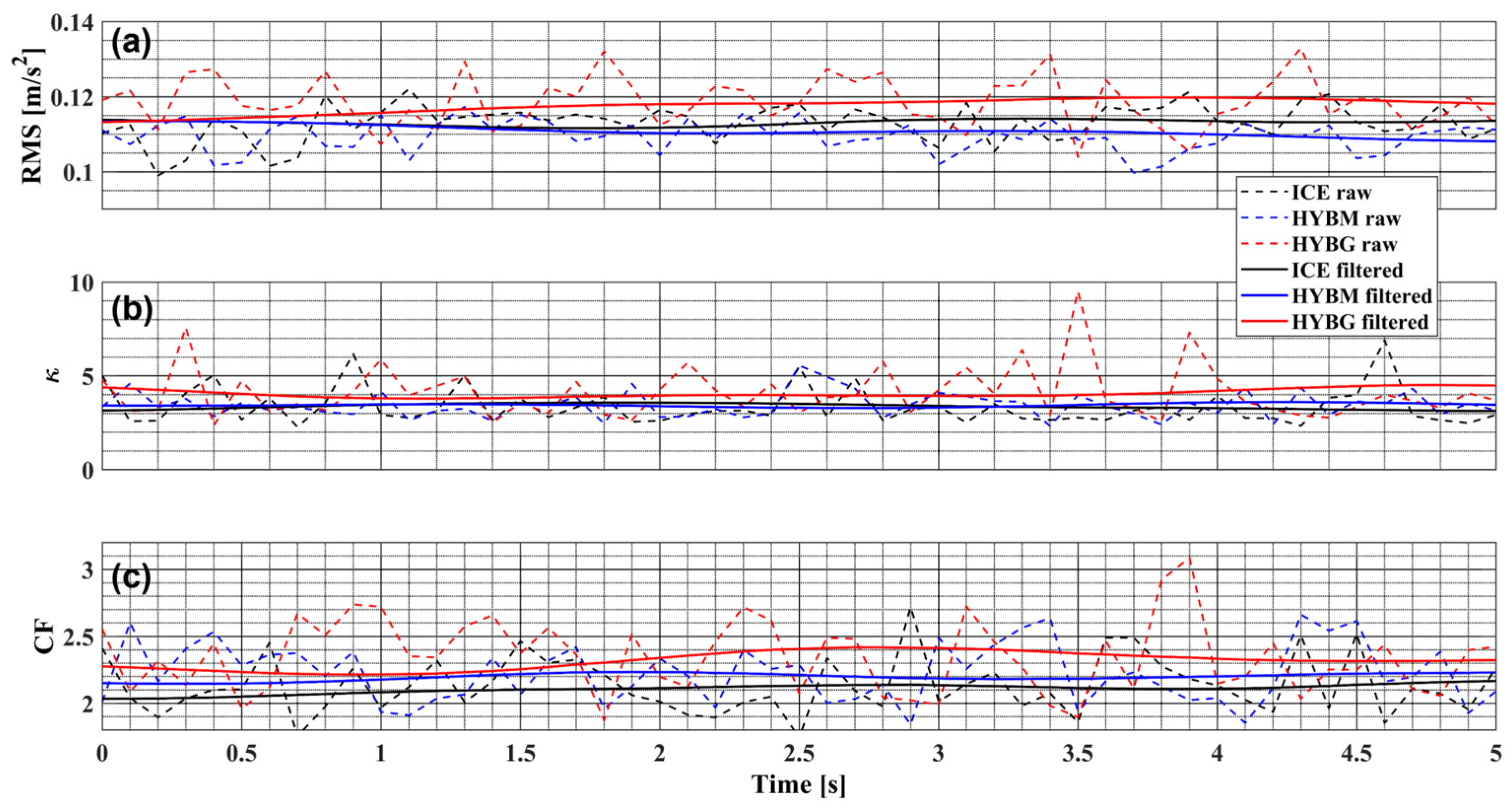
5. Results and Discussion

The acquired signals along the three accelerometer axes, the combined signal, the angular speed, and the propeller torque of a test in the ICE operating mode of the HEPS are shown in Figure 5.

The test in Figure 5 was performed at a constant angular speed and torque (Figure 5a,b), and the result signal (Figure 5f) was always positive.

To completely describe the system dynamics, 22 time-features were calculated from the combined signals to describe the HEPS’ dynamic behavior in the three configurations when the equilibrium point was inside the ±5% limits of the propeller torque curve. The raw indexes were very noisy and overlapped in the three HEPS operating modes if the EM torque tended to zero: using a lowpass FIR filter, it was possible to improve the ICE, HYBM and HYBG differences. As an example, Figure 6 shows the angular speed, the total torque, and the EM torque in the three HEPS operating modes when the EM torque was around ±5 Nm, while Figure 7 shows the raw and filtered trends of three indexes (RMS, kurtosis, and crest factor) to clarify the filter importance.

Figure 6 shows the coincidence between the three HEPS operating point configurations and how the EM torque contribution was negligible compared with that of the ICE. For this reason, the raw indices in Figure 7 tend to overlap, but using the FIR filter, the differentiation between the three different configurations could be improved.

The 22 filtered time-features were divided into 50% training, 20% validation, and 30% test datasets using the Holdout method. The three datasets were standardized, and PCA analysis was performed on the training dataset. The PCA analysis results are shown in Figure 8.

Analyzing the trend of the total variance explained as a function of 22 PCA cumulative number components (as the 22 filtered time-features) in Figure 8a, the first three principal directions were found to explain 96.10% of the original data variance: the first direction explains 69.53%, the second 24.42%, and the third 2.15% (Figure 8b). Since the first three PCs managed to explain over 95% of the index’s total variance, only the first three components were used as input data to train, validate and test the model. The PCA transformation matrix calculated on the training dataset was also used to transform the validation and test datasets.

The FNN model was trained and optimized using Bayesian Optimization to predict the HEPS’ operating mode. The model was only trained with the torque/speed equilibrium point inside the ±5% limit tests. The only used FNN input data were the three components obtained from the PCA analysis. The reduced number of inputs to the model reduced the calculation time of all phases (training, validation, and testing), as well as the optimization time.

Figure 9 shows the last training loss curve and the Bayesian Optimization loss trend, and

Table 1. FNN hyperparameters.

Hyperparameter	Range	Optimized
Input Layer Neurons	/	3
Output Layer Neurons	/	3
Input Layer Activation Function	/	ReLu
Output Layer Activation Function	/	SoftMax
Hidden Layer	$1÷3$	3
First Hidden Layer Neurons	$1÷300$	145
Second Hidden Layer Neurons	$1÷300$	32
Third Hidden Layer Neurons	$1÷300$	204
Hidden Layer Activation Function	ReLu, Tanh, Softmax, Sigmoid	Tanh
Regularization Parameter	${10}^{-5}÷1$	$2.2251\times {10}^{-5}$
FNN Train Epoch	/	1000
FNN Train Loss Function	/	MSE
Batch Size	/	32
Learning Rate	${10}^{-6}÷{10}^{-1}$	$8.421\times {10}^{-3}$
Optimization Algorithm	/	Quasi-Newton BFGS

reports the optimized FNN hyperparameters.

The model was tested using the remaining dataset, which was never used during the training phase. In Figure 10, the confusion matrix of the test phase is shown.

The confusion matrix showed that the model had a total accuracy of 97.44%, with the highest classification error of 4.4% for the ICE class. The model was not tested with the same number of the three classes, so the total accuracy was not a simple mean.

The signals acquired with the torque/speed equilibrium points outside the $\pm 5$% limits were processed like the training, validation, and testing datasets. These new inputs were used to test the model, and the accuracy was 29.41%: the accuracy decrease underlines the model’s inability to predict the correct class when the equilibrium point was outside the limits.

A logical vector was built to monitor the position of the speed–torque equilibrium point and detect changes in air properties. The RMS value was then computed from this vector every second to track the equilibrium point location within the angular speed–torque plane. To demonstrate the monitor technique’s validity, Figure 10 reports the results of a final test with a total duration of 60 s and an angular speed range from 1000 to 2500 rpm in different HEPS operating modes: starting from second 26, the equilibrium point moved outside the $\pm 5$% limits.

In Figure 11, it is impossible to detect the equilibrium point leakage: the parameter test did not show any difference between the range from 0 to 26 s and the fault zone from 26 to 60 s.

Figure 12 shows the angular speed–torque plane and the RMS trend during the final test.

Figure 12a shows the test propeller torque curve deviation from the ±5% limits, as highlighted in the red zone, which was not identified by the parameters reported in Figure 11. Figure 12b reports the RMS trends:

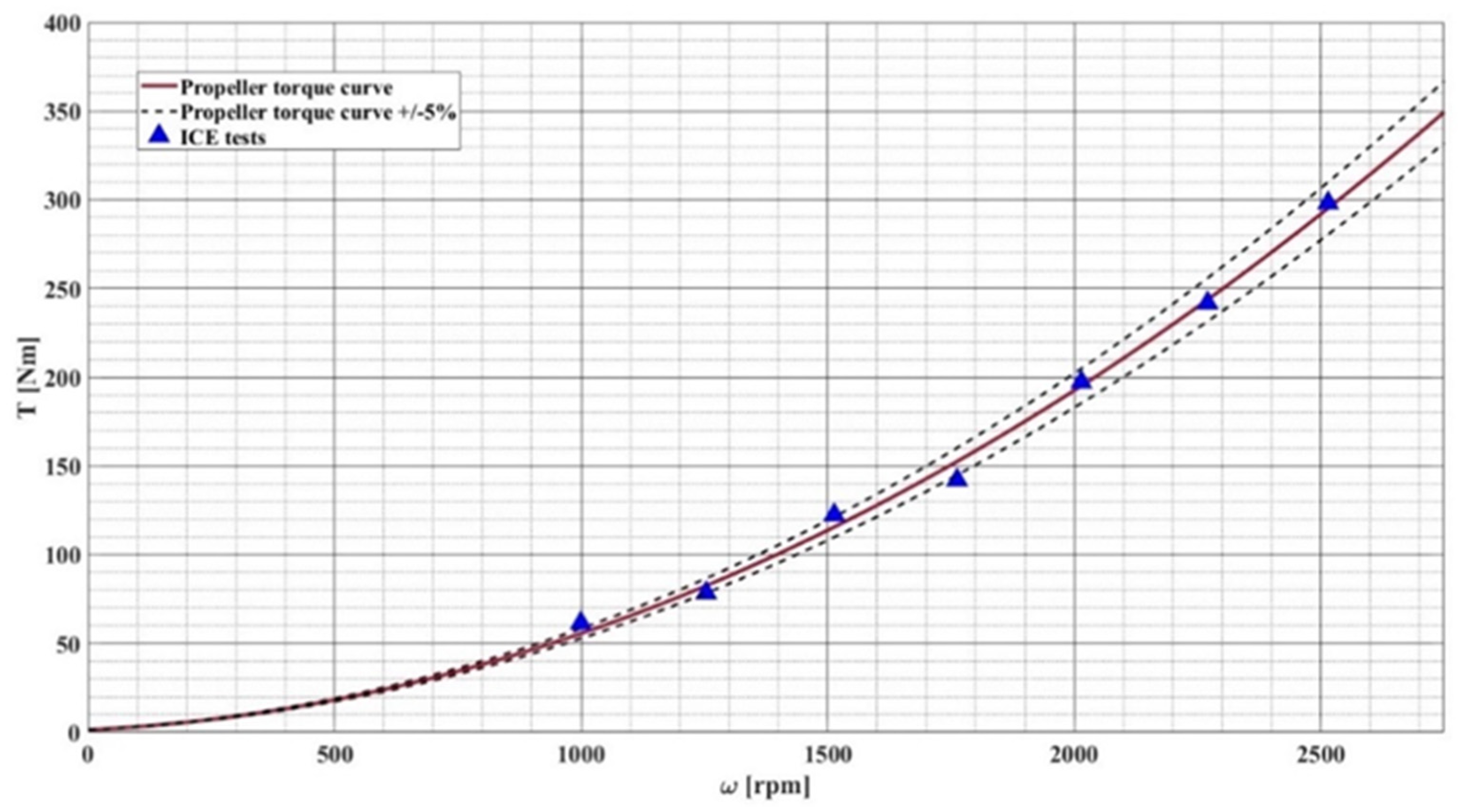
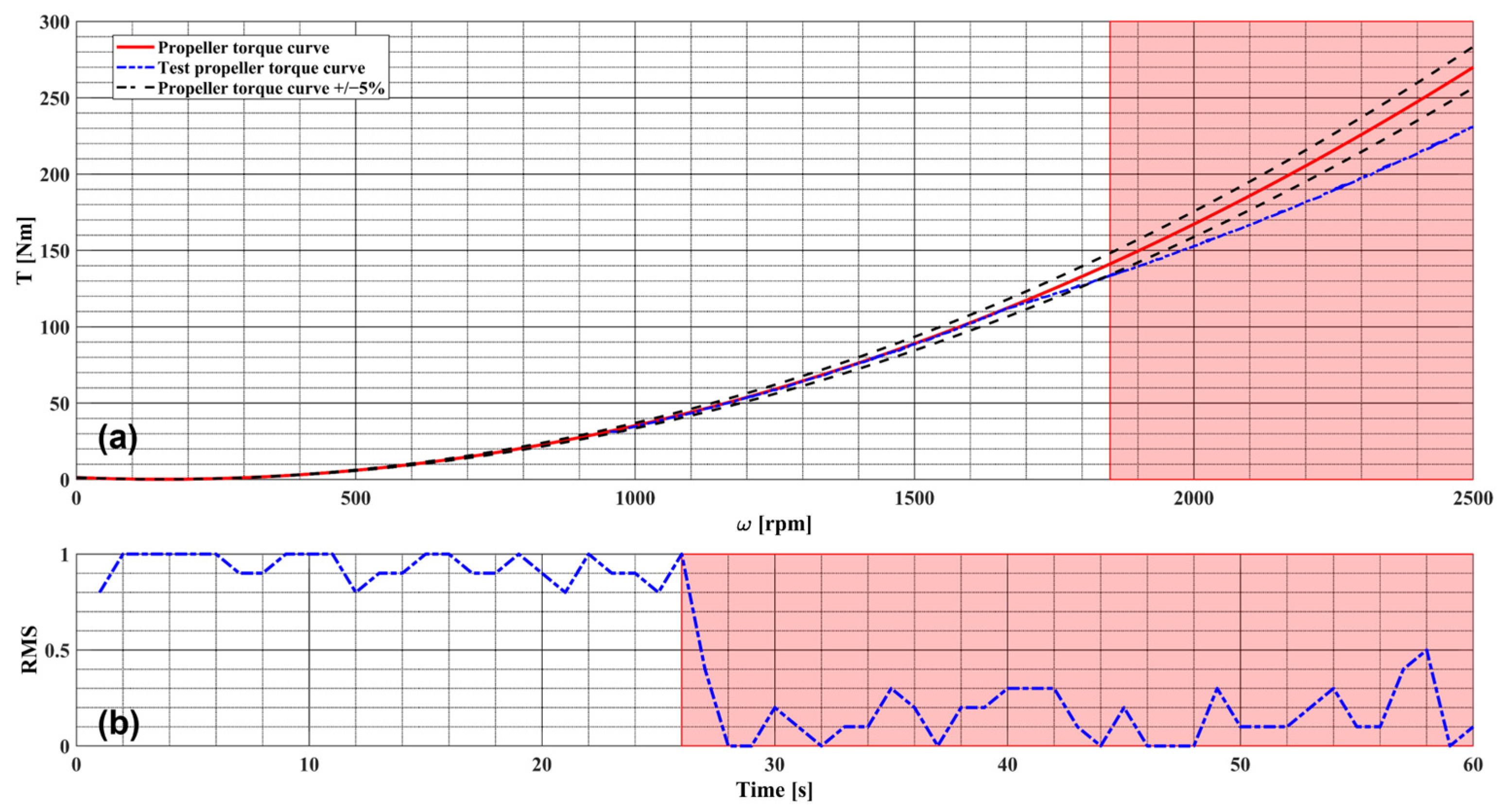
• When the propeller torque curve was inside the ±5% limits (range 0–25 s), the RMS trend was toward 1 with a mean of 0.94;
• When the propeller torque curve was outside the ±5% limits (range 26–60 s), the RMS value was toward 0 with a mean of 0.29.

The clear difference between the RMS values in the range from 0 to 26 s and the remaining test part demonstrates the statistical index monitor’s capability to detect the torque/speed equilibrium point leakage from the ±5% limits of a propeller torque curve.

6. Conclusions

The application of accelerometric signal analysis to monitor the torque/speed equilibrium points of HEPS is not widely documented in the existing literature. In this study, a novel equilibrium point position accelerometric-signal-based monitoring technique for an aircraft HEPS was presented. The experimental tests were conducted in two different cases:

• The equilibrium point position was inside the ±5% limits of the propeller torque curve;
• The equilibrium point position was outside the ±5% limits of the propeller torque curve.

The three-axis accelerometric signals were combined, while time-features were calculated and filtered to discriminate the HEPS’ operating mode. Using the Holdout method, training, validation, and testing datasets were obtained, standardized, and finally transformed and reduced using PCA. An FNN was trained and optimized with only the equilibrium point position inside the ±5% limit tests. The ML model predicted the HEPS’ operating mode with a total accuracy of 97.44% in the test phase. Subsequently, the FFN is tested with inputs derived from equilibrium point positions outside the ±5% limits, showing a decrease in total accuracy to 29.41%. Starting from the classification results, a logical vector was realized, and an RMS value was calculated. The experimental tests demonstrated the statistical index’s ability to monitor equilibrium point leakage within a ±5% limits due to air property changes.

The approach presented in this paper could represent an innovative contribution to the field, introducing a potentially new methodology for monitoring HEPS. The proposed signal processing method has a low computational cost (statistical index and filtering) and has already been implemented in real time in other literature works. Other techniques only have higher costs in the first stage (FNN training and optimization) or in the transformation matrix calculation (PCA analysis). The proposed method can be applied to all kinds of HEPS because it is based only on accelerometric signals. The future goal is to improve the presented technique and implement it onboard to monitor the equilibrium point position in the angular speed–torque plane in real time.

References

1. Tiboni, M.; Remino, C.; Bussola, R.; Amici, C. A review on vibration-based condition monitoring of rotating machinery. Appl. Sci. 2022, 12, 972. [Google Scholar] [CrossRef]
2. Aherwar, A. An investigation on gearbox fault detection using vibration analysis techniques: A review. Aust. J. Mech. Eng. 2012, 10, 169–183. [Google Scholar] [CrossRef]
3. Kirankumar, M.V.; Lokesha, M.; Kumar, S.; Kumar, A. Review on Condition Monitoring of Bearings using vibration analysis techniques. In IOP Conference Series: Materials Science and Engineering; IOP Publishing: Bristol, UK, 2018; Volume 376, p. 012110. [Google Scholar]
4. Mohd Ghazali, M.H.; Rahiman, W. Vibration analysis for machine monitoring and diagnosis: A systematic review. Shock Vib. 2021, 2021, 9469318. [Google Scholar] [CrossRef]
5. Bianchini, A.; Rossi, J.; Antipodi, L. A procedure for condition-based maintenance and diagnostics of submersible well pumps through vibration monitoring. Int. J. Syst. Assur. Eng. Manag. 2018, 9, 999–1013. [Google Scholar] [CrossRef]
6. Niola, V.; Savino, S.; Quaremba, G.; Cosenza, C.; Spirto, M.; Nicolella, A. Study on the dispersion of lubricant film from a cylindrical gearwheels with helical teeth by vibrational analysis. WSEAS Trans. Appl. Theor. Mech. 2021, 16, 274–282. [Google Scholar] [CrossRef]
7. Cosenza, C.; Malfi, P.; Nicolella, A.; Niola, V.; Savino, S.; Spirto, M. Experimental approach to study the tribological state of gearwheel through vision devices. Int. J. Mech. Control 2023, 24, 61–68. [Google Scholar]
8. McFadden, P.D.; Toozhy, M.M. Application of synchronous averaging to vibration monitoring of rolling element bearings. Mech. Syst. Signal Process. 2000, 14, 891–906. [Google Scholar] [CrossRef]
9. Hu, C.; Smith, W.A.; Randall, R.B.; Peng, Z. Development of a gear vibration indicator and its application in gear wear monitoring. Mech. Syst. Signal Process. 2016, 76, 319–336. [Google Scholar] [CrossRef]
10. De Azevedo, H.D.; de Arruda Filho, P.H.; Araújo, A.M.; Bouchonneau, N.; Rohatgi, J.S.; De Souza, R.M. Vibration monitoring, fault detection, and bearings replacement of a real wind turbine. J. Braz. Soc. Mech. Sci. Eng. 2017, 39, 3837–3848. [Google Scholar] [CrossRef]
11. Ni, Q.; Ji, J.C.; Feng, K.; Halkon, B. A novel correntropy-based band selection method for the fault diagnosis of bearings under fault-irrelevant impulsive and cyclostationary interferences. Mech. Syst. Signal Process. 2021, 153, 107498. [Google Scholar] [CrossRef]
12. Niola, V.; Quaremba, G.; Avagliano, V. Vibration monitoring of gear transmission. In WSEAS International Conference. Proceedings. Mathematics and Computers in Science and Engineering (No. 5); WSEAS: Athens, Greece, 2009. [Google Scholar]
13. Bartelmus, W.; Zimroz, R. Vibration condition monitoring of planetary gearbox under varying external load. Mech. Syst. Signal Process. 2009, 23, 246–257. [Google Scholar] [CrossRef]
14. Niola, V.; Quaremba, G. The Gear Whine Noise: The influence of manufacturing process on vibro-acoustic emission of gear-box. In Proceedings of the 10th WSEAS International Conference, Recent Researches in Communications, Automation, Signal Processing, Nanotechnology, Astronomy and Nuclear Physics, Athens, Greece, 20 February 2011. [Google Scholar]
15. Romagnuolo, L.; Frosina, E.; Amoresano, A.; Quaremba, G.; Spirto, M.; Senatore, A. Instability measurement of cavitation conditions in a spool valve through the definition of a cavitation instability index. Flow Meas. Instrum. 2023, 91, 102366. [Google Scholar] [CrossRef]
16. Casoli, P.; Pastori, M.; Scolari, F.; Rundo, M. A vibration signal-based method for fault identification and classification in hydraulic axial piston pumps. Energies 2019, 12, 953. [Google Scholar] [CrossRef]
17. Saxena, A.; Saad, A. Evolving an artificial neural network classifier for condition monitoring of rotating mechanical systems. Appl. Soft Comput. 2007, 7, 441–454. [Google Scholar] [CrossRef]
18. Praveenkumar, T.; Sabhrish, B.; Saimurugan, M.; Ramachandran, K.I. Pattern recognition based on-line vibration monitoring system for fault diagnosis of automobile gearbox. Measurement 2018, 114, 233–242. [Google Scholar] [CrossRef]
19. Wang, W.; Ismail, F.; Golnaraghi, F. A neuro-fuzzy approach to gear system monitoring. IEEE Trans. Fuzzy Syst. 2004, 12, 710–723. [Google Scholar] [CrossRef]
20. Wang, W. An enhanced diagnostic system for gear system monitoring. IEEE Trans. Syst. Man Cybern. Part B 2008, 38, 102–112. [Google Scholar] [CrossRef]
21. Zhang, M.; Cui, H.; Li, Q.; Liu, J.; Wang, K.; Wang, Y. An improved sideband energy ratio for fault diagnosis of planetary gearboxes. J. Sound Vib. 2021, 491, 115712. [Google Scholar] [CrossRef]
22. Zhan, Y.; Makis, V. A robust diagnostic model for gearboxes subject to vibration monitoring. J. Sound Vib. 2006, 290, 928–955. [Google Scholar] [CrossRef]
23. Shao, Y.; Mechefske, C.K. Gearbox vibration monitoring using extended Kalman filters and hypothesis tests. J. Sound Vib. 2009, 325, 629–648. [Google Scholar] [CrossRef]
24. Siano, D.; Panza, M.A. Diagnostic method by using vibration analysis for pump fault detection. Energy Procedia 2018, 148, 10–17. [Google Scholar] [CrossRef]
25. Feng, K.; Ji, J.C.; Ni, Q.; Beer, M. A review of vibration-based gear wear monitoring and prediction techniques. Mech. Syst. Signal Process. 2023, 182, 109605. [Google Scholar] [CrossRef]
26. Tang, Z.; Guo, J.; Wang, Y.; Xu, W.; Bao, Y.; He, J.; Zhang, Y. Automated seismic event detection considering faulty data interference using deep learning and Bayesian fusion. Comput. Aided Civ. Infrastruct. Eng. 2024. Available online: https://onlinelibrary.wiley.com/doi/full/10.1111/mice.13377 (accessed on 26 December 2024).
27. Wang, H.; Xu, J.; Sun, C.; Yan, R.; Chen, X. Intelligent fault diagnosis for planetary gearbox using time-frequency representation and deep reinforcement learning. IEEE/ASME Trans. Mechatron. 2021, 27, 985–998. [Google Scholar] [CrossRef]
28. Li, Z.; Yan, X.; Wang, X.; Peng, Z. Detection of gear cracks in a complex gearbox of wind turbines using supervised bounded component analysis of vibration signals collected from multi-channel sensors. J. Sound Vib. 2016, 371, 406–433. [Google Scholar] [CrossRef]
29. Feng, K.; Smith, W.A.; Randall, R.B.; Wu, H.; Peng, Z. Vibration-based monitoring and prediction of surface profile change and pitting density in a spur gear wear process. Mech. Syst. Signal Process. 2022, 165, 108319. [Google Scholar] [CrossRef]
30. Laissaoui, A.; Bouzouane, B.; Miloudi, A.; Hamzaoui, N. Perceptive analysis of bearing defects (Contribution to vibration monitoring). Appl. Acoust. 2018, 140, 248–255. [Google Scholar] [CrossRef]
31. Loutas, T.H.; Sotiriades, G.; Kalaitzoglou, I.; Kostopoulos, V. Condition monitoring of a single-stage gearbox with artificially induced gear cracks utilizing on-line vibration and acoustic emission measurements. Appl. Acoust. 2009, 70, 1148–1159. [Google Scholar] [CrossRef]
32. Delvecchio, S.; Bonfiglio, P.; Pompoli, F. Vibro-acoustic condition monitoring of Internal Combustion Engines: A critical review of existing techniques. Mech. Syst. Signal Process. 2018, 99, 661–683. [Google Scholar] [CrossRef]
33. Kar, C.; Mohanty, A.R. Monitoring gear vibrations through motor current signature analysis and wavelet transform. Mech. Syst. Signal Process. 2006, 20, 158–187. [Google Scholar] [CrossRef]
34. Kar, C.; Mohanty, A.R. Vibration and current transient monitoring for gearbox fault detection using multiresolution Fourier transform. J. Sound Vib. 2008, 311, 109–132. [Google Scholar] [CrossRef]
35. Amoresano, A.; Niola, V.; Quaremba, A. A sensitive methodology for the EGR optimization: A perspective study. Int. Rev. Mech. Eng. 2012, 6, 1082–1088. [Google Scholar]
36. Zhang, L.; Lin, Y.; Yang, X.; Chen, T.; Cheng, X.; Cheng, W. From sample poverty to rich feature learning: A new metric learning method for few-shot classification. IEEE Access 2024, 12, 124990–125002. [Google Scholar] [CrossRef]
37. Niola, V.; Rossi, C. Video acquisition of a robot arm trajectories in the work space. WSEAS Trans. Comput. 2005, 4, 830–836. [Google Scholar]
38. Niola, V.; Rossi, C.; Savino, S.; Troncone, S. An underactuated mechanical hand: A first prototype. In Proceedings of the 2014 23rd International Conference on Robotics in Alpe-Adria-Danube Region (RAAD), Smolenice, Slovakia, 3–5 September 2014; pp. 1–6. [Google Scholar]
39. Malfi, P.; Nicolella, A.; Spirto, M.; Cosenza, C.; Niola, V.; Savino, S. Motion sensing study on a mobile robot through simulation model and experimental tests. WSEAS Trans. Appl. Theor. Mech. 2022, 17, 79–85. [Google Scholar] [CrossRef]
40. Penta, F.; Rossi, C.; Savino, S. An underactuated finger for a robotic hand. Int. J. Mech. Control 2014, 15, 63–68. [Google Scholar]
41. Ma, S.; Wang, S.; Zhang, C.; Zhang, S. A method to improve the efficiency of an electric aircraft propulsion system. Energy 2017, 140, 436–443. [Google Scholar] [CrossRef]
42. Wang, S.; Zhang, S.; Ma, S. An energy efficiency optimization method for fixed pitch propeller electric aircraft propulsion systems. IEEE Access 2019, 7, 159986–159993. [Google Scholar] [CrossRef]
43. Song, Z.; Liu, C. Energy efficient design and implementation of electric machines in air transport propulsion system. Appl. Energy 2022, 322, 119472. [Google Scholar] [CrossRef]
44. Epstein, A.H.; O’Flarity, S.M. Considerations for reducing aviation’s CO2 with aircraft electric propulsion. J. Propuls. Power 2019, 35, 572–582. [Google Scholar] [CrossRef]
45. Mercer, C.; Haller, W.; Tong, M. Adaptive engine technologies for aviation CO2 emissions reduction. In Proceedings of the 42nd AIAA/ASME/SAE/ASEE Joint Propulsion Conference & Exhibit, Sacramento, CA, USA, 9–12 July 2006; p. 5105. [Google Scholar]
46. Kuśmierek, A.; Galiński, C.; Stalewski, W. Review of the hybrid gas-electric aircraft propulsion systems versus alternative systems. Prog. Aerosp. Sci. 2023, 141, 100925. [Google Scholar] [CrossRef]
47. Fentaye, A.D.; Zaccaria, V.; Kyprianidis, K. Aircraft engine performance monitoring and diagnostics based on deep convolutional neural networks. Machines 2021, 9, 337. [Google Scholar] [CrossRef]
48. Krajček, K.; Nikolić, D.; Domitrović, A. Aircraft performance monitoring from flight data. Teh. Vjesn. 2015, 22, 1337–1344. [Google Scholar]
49. Antoni, J.; Griffaton, J.; André, H.; Avendano-Valencia, L.D.; Bonnardot, F.; Cardona-Morales, O.; Castellanos-Dominguez, G.; Daga, A.P.; Leclère, Q.; Vicuña, C.M.; et al. Feedback on the Surveillance 8 challenge: Vibration-based diagnosis of a Safran aircraft engine. Mech. Syst. Signal Process. 2017, 97, 112–144. [Google Scholar] [CrossRef]
50. Herzog, J.P.; Hanlin, J.; Wegerich, S.W.; Wilks, A.D. High performance condition monitoring of aircraft engines. In Turbo Expo: Power for Land, Sea, and Air; ASME: New York, NY, USA, 2005; Volume 46997, pp. 127–135. [Google Scholar]
51. Ghazi, G.; Gerardin, B.; Gelhaye, M.; Botez, R.M. New adaptive algorithm development for monitoring aircraft performance and improving flight management system predictions. J. Aerosp. Inf. Syst. 2020, 17, 97–112. [Google Scholar] [CrossRef]
52. Léonard, O.; Borguet, S.; Dewallef, P. Adaptive estimation algorithm for aircraft engine performance monitoring. J. Propuls. Power 2008, 24, 763–769. [Google Scholar] [CrossRef]
53. Bieber, M.; Verhagen, W.J.; Cosson, F.; Santos, B.F. Generic Diagnostic Framework for Anomaly Detection—Application in Satellite and Spacecraft Systems. Aerospace 2023, 10, 673. [Google Scholar] [CrossRef]
54. Fornaro, E.; Cardone, M.; Dannier, A. A comparative assessment of hybrid parallel, series, and full-electric propulsion systems for aircraft application. IEEE Access 2022, 10, 28808–28820. [Google Scholar] [CrossRef]
55. Fornaro, E.; Cardone, M.; Dannier, A. Hybrid Electric Aircraft Model Based on ECMS Control. In Proceedings of the 2022 International Symposium on Power Electronics, Electrical Drives, Automation and Motion (SPEEDAM), Sorrento, Italy, 22–24 June 2022; pp. 865–870. [Google Scholar]
56. Niola, V.; Fornaro, E.; Spirto, M.; Malfi, P.; Melluso, F. A Comparison Between Different Hybrid Electric Propulsion System Configurations by Means of Vibrational Analysis and Fuel Consumption. In Proceedings of the International Conference of IFToMM ITALY; Springer: Cham, Switzerland, 2024; pp. 452–460. [Google Scholar]
57. McCormick, B.W. Aerodynamics, Aeronautics, and Flight Mechanics; John Wiley & Sons: Hoboken, NJ, USA, 1994. [Google Scholar]
58. Neuvo, Y.; Cheng-Yu, D.; Mitra, S. Interpolated finite impulse response filters. IEEE Trans. Acoust. Speech Signal Process. 1984, 32, 563–570. [Google Scholar] [CrossRef]
59. Kohavi, R. A study of cross-validation and bootstrap for accuracy estimation and model selection. IJCAI 1995, 14, 1137–1145. [Google Scholar]
60. Bishop, C.M. Pattern Recognition and Machine Learning; Springer: New York, NY, USA, 2006; Volume 2, pp. 5–43. [Google Scholar]
61. Jolliffe, I.T. Principal Component Analysis for Special Types of Data; Springer: New York, NY, USA, 2002; pp. 338–372. [Google Scholar]
62. Zeng, L. Prediction and classification with neural network models. Sociol. Methods Res. 1999, 27, 499–524. [Google Scholar] [CrossRef]
63. Féraud, R.; Clérot, F. A methodology to explain neural network classification. Neural Netw. 2002, 15, 237–246. [Google Scholar] [CrossRef]
64. Joy, T.T.; Rana, S.; Gupta, S.; Venkatesh, S. Batch Bayesian optimization using multi-scale search. Knowl. Based Syst. 2020, 187, 104818. [Google Scholar] [CrossRef]
65. Joy, T.T.; Rana, S.; Gupta, S.; Venkatesh, S. Hyperparameter tuning for big data using Bayesian optimisation. In Proceedings of the 2016 23rd International Conference on Pattern Recognition (ICPR), Cancun, Mexico, 4–8 December 2016; pp. 2574–2579. [Google Scholar]
66. Večeř, P.; Kreidl, M.; Šmíd, R. Condition indicators for gearbox condition monitoring systems. Acta Polytech. 2005, 45, 35–43. [Google Scholar] [CrossRef] [PubMed]
67. Ram, B.; Mishra, S.K.; Lai, K.K.; Rajković, P. Quantum Limited Memory Broyden Fletcher Goldfarb Shanno Method. In Unconstrained Optimization and Quantum Calculus; Springer Nature: Singapore, 2024; pp. 125–138. [Google Scholar]
Figure 1. Hybrid electric architecture for aircraft application.
Applsci 15 02135 g001
Figure 2. Propeller torque curve.
Applsci 15 02135 g002
Figure 3. Training, validation, and testing dataset partition workflow.
Applsci 15 02135 g003
Figure 4. Model training, optimization, and testing workflow.
Applsci 15 02135 g004
Figure 5. ICE mode test: (a) angular speed, (b) total torque, (c) x-axis vibrational signal, (d) y-axis vibrational signal, (e) z-axis vibrational signal, and (f) combined signal.
Applsci 15 02135 g005
Figure 6. Parameter test trends: (a) angular speed, (b) total torque, and (c) EM torque.
Applsci 15 02135 g006
Figure 7. Raw and filtered index trends: (a) RMS, (b) kurtosis, (c) crest factor.
Applsci 15 02135 g007
Figure 8. PCA analysis results: (a) total explained variance and (b) single PC component explained variance.
Applsci 15 02135 g008
Figure 9. Loss curves: (a) last FFN loss curve and (b) Bayesian Optimization loss curve.
Applsci 15 02135 g009
Figure 10. Confusion matrix.
Applsci 15 02135 g010
Figure 11. Final test parameters trends with the equilibrium point outside the ± 5 % limits highlighted in red: (a) propeller torque, (b) Electric Machine torque, and (c) angular speed.
Applsci 15 02135 g011
Figure 12. Final test results with the equilibrium point outside the ± 5 % limits highlighted in red: (a) propeller torque curve trend in the angular speed–torque curve plane and (b) RMS trend.
Applsci 15 02135 g012