1. Introduction
With the rise of smart technologies and the Smart Cities concept, cities are increasingly focusing on the digitization of their infrastructure and more efficient management of urban environments. A key role in this process is played by the 3D mapping of infrastructure using advanced technologies, such as laser scanning, which enables the creation of accurate and detailed digital models of urban structures. These models are essential for the development of so-called Digital Twins [
1,
2], which are digital replicas of the physical world, allowing for comprehensive analyses, simulations, and optimizations [
3,
4]. In this context, Žiar nad Hronom, as one of Slovakia’s industrial centers, has decided to adopt modern methods of infrastructure mapping using terrestrial laser scanning (TLS) and mobile laser scanning (MLS) technologies. These advanced non-contact methods allow for the acquisition of highly accurate data without direct manipulation of the physical environment, minimizing disruption to the infrastructure while increasing process efficiency.
The collection of spatial data using non-contact methods is carried out using modern technology composed of various types of sensors. Among non-contact methods, the TLS method has experienced significant growth in recent times. TLS is used to survey single objects or small areas of land. It is characterized by its high measurement speed and ability to capture a large density of points in a point cloud. It can be employed to measure the position and shapes of various asymmetrical and irregular objects. Thanks to its level of detail, speed, and number of captured points, it is possible to create an accurate digital 3D model of objects. TLS determines the spatial coordinates X, Y, and Z of points based on the spatial polar method. Application of TLS can be seen in fields such as engineering and construction [
5,
6], industry [
7,
8,
9], and land mapping [
10,
11].
MLS is a new technology capable of capturing three-dimensional data from surrounding objects. Using the most modern sensors, the resulting point clouds capture object details with sufficient accuracy and density. MLS measurements can be carried out while the mobile laser scanner is mounted on various moving mobile platforms (UAV, car, boat), with the positioning system—usually based on a global navigation satellite system (GNSS) and inertial measurement unit (IMU)—tracking the trajectory and position of the scanner to create a 3D point cloud from measured data. Mobile laser scanners consist of data collection sensors and positioning sensors. The data collection sensors primarily include a calibrated Lidar (light detection and ranging) and a set of digital cameras. The Lidar sensor is capable of producing up to 1,000,000 points per second, and the camera set captures up to a 360° horizontal field of view to provide texture and color information for the point cloud, if necessary [
12]. However, these systems are also capable of digitizing complex 3D scenes on the move without GNSS due to simultaneous localization and mapping (SLAM) algorithms [
13,
14,
15]. The SLAM process focuses on mapping an unknown environment and simultaneously locating the sensor system within that environment through signals provided by the sensor. In terms of data quality, these devices typically offer centimeter-level accuracy [
16]. The resolution depends on the scanning speed of the sensor and the distance from the object at any given moment. Several factors determine the type of sensor and platform needed for MLS tasks. These factors include sensor availability, project budget, technical solutions, desired accuracy and density of the point cloud, processing strategies, scene content, and interpretation of the resulting outputs. Using MLS techniques, large datasets of urban objects can be created, and dense, accurate point clouds enable various survey tasks. The MLS method is used for the reconstruction of outdoor scenes and objects that are classified as cultural heritage [
17,
18]. Civil engineering [
19], underground space mapping [
20,
21,
22], detection and inventory of poles, traffic signs, and road objects [
23,
24,
25], as well as light poles, are prime examples of MLS used in urban infrastructure maintenance [
26,
27,
28]. The MLS method is also used for forest inventory [
29,
30,
31] and in agriculture [
32].
When using MLS in urbanized areas, the accuracy of the collected data depends on several factors. One of the key elements to ensure georeferencing and increase the precision of 3D models is the use of ground control points (GCPs) and check points (CPs). These points provide reference coordinates and are essential for precisely aligning scanned data with local or national coordinate systems. They play a critical role in the correction and calibration of data collected during scanning, significantly improving the accuracy and consistency of the resulting 3D models. The implementation of GCPs and CPs helps to minimize errors in georeferencing, which can arise due to the movement of the scanning device, and ensures the consistency and reliability of 3D data throughout the entire mapped area. This integration of GCPs with MLS represents a key technique for effective and accurate mapping of urban structures [
33,
34] in the context of Smart City development and Digital Twins.
This article focuses on the analysis of datasets captured in the city center of Žiar nad Hronom using different laser scanning approaches. A field survey was conducted using the TLS method with the Leica RTC360 terrestrial laser scanner and the MLS method using various mobile platforms at the same time. The second section of the article provides a description and characterization of the study area. The third section addresses the surveying work carried out in the field, describes the fieldwork and the types of different GCPs and CPs, and outlines the technical parameters of all the surveying instruments and tools used. The fourth and fifth sections present the data processing and the results achieved from the field measurements, comparing the different methods based on classification, differences in individual objects, detail and density, and noise. The Discussion section highlights the advantages and disadvantages of the surveying methods used and compares these methods based on noise levels. This section also discusses solutions addressed by other authors on similar issues in their research papers.
5. Results
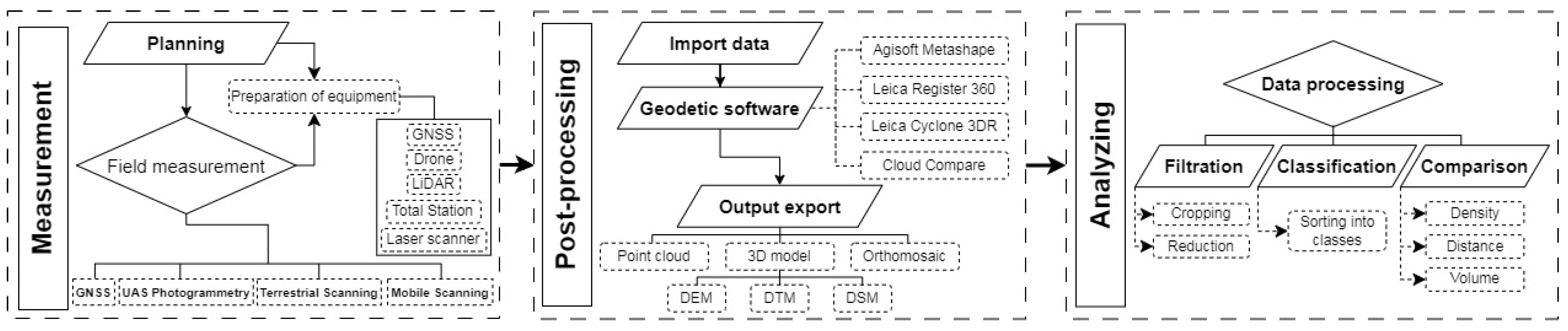
Analyses were conducted using the data acquired by TLS and MLS to compare point clouds based on their classification, shifts in the selected objects, details, and density. Before the actual comparisons, the data were processed into a form where unwanted and redundant points were filtered out from each point cloud. The program Trimble Realworks 12.2 was used for segmenting the point clouds from TLS and MLS, while Leica Cyclone 3DR, Trimble Realworks 12.2, and CloudCompare 2.13 were employed for processing, filtering, visualizing, and comparing the data.
Figure 7 illustrates the optimized workflow diagram from measurement through processing to analysis of the point clouds.
After processing the data from TLS and MLS, dense point clouds were generated, which served as input for further comparisons and analyses. For TLS, the resulting dense point cloud (
Figure 8a) was generated with the Leica Cyclone Register 360 software and contained 916,014,221 points. This point cloud was subsequently classified and filtered. Three different mobile laser scanners were used for the MLS method. The point cloud generated by the mobile scanner Lidaretto contains 119,383,840 points (
Figure 8b) with an overall RMSE accuracy of 3.4 cm on CPs. The resulting point cloud from the mobile laser scanner Stonex X120GO comprises 199,096,585 points (
Figure 8c) with an overall RMSE accuracy of 2.1 cm on CPs. The iPhone 13 Pro with an Emlid scanning kit and a GNSS antenna Reach RX generated a point cloud containing 14,384,860 points (
Figure 8d).
5.1. Analysis of the Automatic and Manual Point Classification
Point classification represents a critical step in point cloud processing, significantly influencing their subsequent use, such as in creating digital terrain models, infrastructure analysis, or other applications. This analysis focuses on the comparison of automatic and manual point classification, emphasizing accuracy, efficiency, and the time demands of both approaches. The evaluation was based on classification classes, the number of correctly classified points, and the total time required for classification. The analysis was conducted in two different software environments—Leica Cyclone 3DR and Trimble Realworks 12.2. These software tools enable point classification using distinct algorithms and workflows. This approach allowed us to identify the advantages and disadvantages of each method, with particular attention paid to factors such as differences in the number of points assigned to specific classification classes and the ability of the automatic classification to handle complex or specific scenarios. The results of this analysis provide a comprehensive overview of the capabilities and limitations of automatic and manual point classification methods in the context of point cloud processing.
In the Leica Cyclone 3DR software, the automatic classification generated five classification classes within approximately 10 min, with each layer automatically assigned by the software from its database. Following the automatic classification, a subsequent manual classification was performed to adjust incorrectly assigned points. During the manual classification process, these points were reassigned to the appropriate classification classes based on their actual characteristics and location. This process helped eliminate errors caused by automatic algorithms, especially in areas with a high level of detail or complex geometry. Manual classification also allowed for the verification of the accuracy of the automatic process and helped determine the extent to which automated procedures could be relied upon in point cloud processing. The most significant discrepancies between automatic and manual classification occurred in the Vegetation class, where more than 740,000 points were reclassified. Most of these points were originally placed in the Building and Ground classes. The software also struggled to detect unnecessary points, often incorrectly placing them in the Building class. These points, due to poor reflection or other factors, were found floating freely in space. Throughout the processing, it became clear that the Ground classification class was the most reliable and accurately defined. The total time for both automatic and manual classification with the Leica Cyclone 3DR software was approximately 75 min.
The same classification process was carried out with the Trimble Realworks software. Automatic classification with this software took only 3 min and divided the points into four classification classes. While the software processed the automatic classification in a very short time, the results reflect this limitation. Subsequently, incorrect points were corrected using manual classification, which took 110 min. In this case, the automatic classification was not as thorough as in the previous processing using Leica Cyclone 3DR. This is evident from the number of points that needed to be reclassified into different classes. Processing with this software was more complex and time-consuming. According to the results, the worst-defined class was Remaining, into which many points from the Vegetation and
Building classes were incorrectly assigned. In many cases, these points should have been clearly placed in other relevant classification classes. The main advantage of this software is the short duration of the automatic classification process. However, its drawbacks include inaccurately classified points, complex and lengthy processing, and the need for extensive manual corrections.
Figure 9 illustrates the building from various perspectives before classification. It then shows the results of automatic and manual classification, highlighting selected objects such as a tree, building, car, and traffic sign. The figure also demonstrates shortcomings and differences in the form of incorrectly classified points on these objects.
Table 6 presents the classification classes and their changes, including increases or decreases in the number of points.
Quantitative evaluation of the classification results was conducted using standard metrics: precision, recall, and F-score (
Table 7). This evaluation was performed in two software environments—Leica Cyclone 3DR and Trimble Realworks 12.2—across the classification classes of ground, vegetation, and buildings. The comparison of automated point cloud classification between Leica Cyclone 3DR and Trimble Realworks reveals significant differences in their performance. For ground point classification, Leica Cyclone 3DR achieved high precision (0.984) and sensitivity (0.962), resulting in an excellent F-score of 0.973. These values suggest that the Leica Cyclone 3DR algorithm can reliably identify ground points with minimal misclassifications. The number of false negatives (FN = 241,423) was relatively low, highlighting the algorithm’s ability to accurately recognize most points in this class. In medium vegetation, Leica Cyclone 3DR demonstrated slightly lower precision (0.854), linked to a higher number of false positives (FP = 750,427). However, sensitivity remained very high (0.988), indicating that most vegetation points were correctly identified. The resulting F-score (0.916) reflects a good balance between precision and sensitivity. For building classification, Leica Cyclone 3DR showed exceptional performance, with a precision of 0.995, a sensitivity of 0.996, and an F-score of 0.995. These values confirm the algorithm’s ability to reliably classify buildings with minimal errors (FP = 228,719, FN = 182,048).
Trimble Realworks achieved very high precision for ground point classification (0.997), indicating minimal points were incorrectly labeled as ground (FP = 13,813). However, its sensitivity was lower (0.905), leading to a higher number of unclassified ground points (FN = 569,521). The resulting F-score (0.949) is still high but falls behind Leica Cyclone 3DR’s performance. For high vegetation, Trimble Realworks delivered weaker results, with low precision (0.554) and very low sensitivity (0.367). This indicates a substantial portion of vegetation points were misclassified (FP = 1,362,413, FN = 2,911,669), resulting in a poor F-score of 0.441. For buildings, Trimble Realworks achieved a precision of 0.952 and a sensitivity of 0.924, leading to an F-score of 0.938. While these results are solid, they fall short of Leica Cyclone 3DR’s performance due to a higher number of misclassifications (FP = 1,931,690, FN = 3,161,156). Overall, Leica Cyclone 3DR provides a better balance between precision and sensitivity across the classification classes of ground, vegetation, and buildings. Trimble Realworks excels in precision for ground points, but its lower sensitivity and weaker performance in vegetation and building classification place it at a disadvantage. These differences highlight the importance of selecting the appropriate tool for point cloud classification based on the specific requirements and focus of the analysis.
5.2. Analysis of the Differences in Point Cloud Based on the Shift on Objects
This section focuses on the analysis of the accuracy and reliability of the TLS and MLS methods by evaluating the shifts on selected objects in an urban environment. For the purposes of this analysis, three types of objects were chosen, each characterized by their structure and stability: a tree, a building, and the mast of a street lamp. These objects provide different surfaces and conditions, ensuring a representative assessment of the accuracy and reliability of both technologies. The goal is to determine the differences between the TLS and MLS methods based on the accuracy of measuring these objects and to identify potential deviations that may affect the resulting point clouds. The analyses on individual objects were carried out using the Leica Cyclone 3DR software. The first object selected for deriving differences between point clouds was a tree, specifically its trunk. The point cloud of the trunk was analyzed from TLS, the Lidaretto mobile laser scanner, and the Stonex X120GO mobile laser scanner (
Figure 10). After filtering unnecessary points, the TLS point cloud contained 6,343,281 points, the Lidaretto mobile laser scanner contained 993,205 points, and the Stonex X120GO point cloud had 457,215 points. For each point cloud, we determined the radius of the tree trunk in the same horizontal cross-section (
Table 8). The TLS trunk radius was 0.493 m; for the Lidaretto, it was 0.451 m; and for the Stonex X120GO, it was 0.507 m. For the mobile laser scanner Lidaretto, the radius deviation from the TLS method, chosen as the reference method, was 0.042 m. For the mobile laser scanner Stonex X120GO, the radius deviation from the reference method was 0.014 m. We also compared the coordinate deviations of the center from the reference method. For the Lidaretto mobile laser scanner, the deviation along the Y-axis was 0.006 m, and along the X-axis, it was 0.003 m. For the Stonex X120GO mobile laser scanner, the deviation along the Y-axis was 0.016 m, and along the X-axis, it was 0.033 m.
The next object chosen for determining the horizontal shifts between point clouds is a building. We observed shifts between the different methods on corners of the building (
Figure 11). In this case, the point cloud obtained using the TLS method with a Leica RTC360 was chosen as the reference. This point cloud was compared with point clouds obtained using the Lidaretto mobile laser scanner, the Stonex X120GO mobile laser scanner, and a combined setup of an iPhone 13 Pro with an Emlid scanning kit and a GNSS antenna Reach RX. A horizontal cross-section of the building was taken at the same height for all the point clouds. In a 2D horizontal plane, the approximated lines define corners as their intersections.
Table 9 shows the shifts and differences between the MLS point clouds compared to the reference TLS data at the corners of the building. The smallest difference was detected at point B when compared with the point cloud from the Stonex X120GO, with a value of 0.9 cm. The largest deviation was found when comparing the point cloud from the Lidaretto at point A, with a value of 10 cm. The best deviations in the comparison between the reference point cloud and the MLS point cloud were achieved with the Stonex X120GO mobile laser scanner, with an average deviation of 3.0 cm for the building. We also compared the MLS point clouds with the reference TLS point cloud based on the cross-section area. In this case, the best result was achieved by the Lidaretto point cloud, with an area only 0.2 m
2 smaller than the building’s cross-section area obtained using the TLS method.
The final object for the horizontal differences derived between point clouds is the mast of a street lamp. Three cross-sections were made on the lamp: one at a height of 1 m from the ground surface and the other two at heights of 3 m and 5 m from the ground surface.
Figure 12 shows the point clouds from each method used in the selected cross-sections.
The individual point clouds were analyzed based on the number of points, radius, and shift. The reference method in this case was the point cloud obtained using the TLS method. In the first analysis, the lowest cross-section, point clouds from the mobile laser scanner Lidaretto, the mobile laser scanner Stonex X120GO, and the iPhone 13 Pro with an Emlid scanning kit and a GNSS antenna Reach RX were analyzed. For the TLS method, the first section consisted of 647 points, and the radius was 0.053 m. Using the mobile laser scanner Stonex X120GO, the first section contained 63 points, with a lamp radius of 0.076 m and a shift from the reference method of 3.27 cm. Using the mobile laser scanner Lidaretto, the first section contained only 13 points, with a lamp radius of 0.063 m and a shift of 3.47 cm. The closest match to the radius of the reference method was achieved by the section from the combined setup of the iPhone 13 Pro with an Emlid scanning kit and a GNSS antenna Reach RX, with a deviation of only 4 mm. However, this section exhibited the largest shift compared to the reference method, specifically 6.56 cm. For the remaining two cross-sections, no data were available from the iPhone 13 Pro with an Emlid scanning kit and a GNSS antenna Reach RX. In the middle section, the deviation in radius for the mobile laser scanner Stonex X120GO was 1.2 cm, with a shift of 1.48 cm. For the mobile laser scanner Lidaretto, the radius deviation was smaller, at just 5 mm, but the shift from the reference method was larger, specifically 2.41 cm. In the third, highest cross-section, the Leica RTC360 produced 176 points and a radius of 0.034 m. In this section, both the radius deviation and the shift of the section were better using the mobile laser scanner Lidaretto.
5.3. Analysis of the Laser Scanning Methods Based on Detail and Density
The density of a point cloud is one of the key parameters influencing the quality and usability of 3D models, as it directly relates to the resolution and accuracy of the resulting data. Our analysis examined point density along the trajectories of selected scanning systems, enabling a better understanding of the distribution and variability of density depending on the position and scanning conditions. The point density for the individual methods was assessed over an area of 504 m
2. Within this area, the point cloud obtained by the TLS method and Leica RTC360 device contained 22,334,716 points, while the mobile laser scanner Stonex X120GO produced 3,932,775 points, and the Lidaretto mobile laser scanner recorded 1,231,288 points. Using the TLS method, point density near the scanner’s positions reached over 80,000 points/m
2. With the MLS method, the trajectory closely followed building walls and other significant objects. The Stonex X120GO mobile laser scanner achieved point densities exceeding 20,000 points/m
2 along the trajectory, while the Lidaretto scanner recorded densities of over 3000 points/m
2 (
Figure 13).
For each surveying method, a histogram based on the point density was created, providing a graphical representation of the point distribution within the point cloud in the same area unit. This approach allows for the identification of areas with higher or lower density and highlights factors that may influence these differences, such as the scanning unit’s movement speed, distance from the objects, or obstacles in the terrain. The histogram was generated with CloudCompare software using the Surface Density function, which calculates the number of neighboring points divided by the area of the neighborhood with a radius of 1 cm. Histograms for the datasets from the Leica RTC360, Stonex X120GO, and Lidaretto are shown in
Figure 14, illustrating the general differences in point cloud density among the scanning instruments used. The TLS method achieves an average point density of 54,798 points/m
2, approximately five times higher than the mobile laser scanner Stonex X120GO, which has an average density of 10,652 points/m
2. The lowest point density is observed with the Lidaretto mobile laser scanner, which has an average density of 2802 points/m
2—around 20 times less than that of the TLS method.
The surveying methods used in our study area were also tested in terms of noise. One of the key parameters in analyzing data obtained from laser scanning is noise, which represents an undesirable impact on the accuracy and quality of point clouds. We tested the noise on the wall of a selected building. In
Figure 15, we can observe that the TLS method resulted in the smallest distance between points, contributing to higher data collection accuracy and lower noise levels compared to MLS methods. The average noise value for the TLS method was 0.3 cm. Noise in TLS manifests as random point deviations in the point cloud caused by external factors such as the surface properties of the scanned objects. Compared to the MLS method, where noise levels were higher, TLS showed a significant advantage in that the noise was kept to a minimum in environments with restricted movement and enclosed spaces. Noise in the MLS method mainly arises due to the continuous movement of the scanning device during data collection. The average noise width for the mobile laser scanner Stonex X120GO reached a value of 2.0 cm. Furthermore, urban environments, which often include various moving objects such as cars, pedestrians, or trees swaying in the wind, can contribute to higher noise levels in the recorded data. When using the mobile laser scanner Lidaretto, noise-filtering software was applied to eliminate redundant points and improve the quality of the point clouds, although this came at the cost of reduced point density and local accuracy. The average noise value for this Lidaretto dataset reached 0.5 cm. When using the mobile laser scanner Stonex X120GO, we observed higher noise levels compared to other MLS devices, which could be attributed to several factors, including scanner movement, complex trajectories, and environmental conditions during the measurement process. The average noise level reached 0.8 cm.
6. Discussion
Based on our results, we focused on a deeper evaluation of the advantages and disadvantages of the TLS and MLS methods. We analyzed parameters such as accuracy, efficiency, and the applicability of TLS and MLS in urban environments, with particular attention to noise in the collected data and methods for its minimization. To compare our results, this section draws on the results of previous studies that have addressed similar issues. We compare achieved accuracy, data structure, and point cloud density with studies conducted in similar urbanized areas, allowing us to better understand the benefits and limitations of TLS and MLS.
The greatest advantage of the TLS method is the high accuracy and detail of the data. TLS provides highly precise measurements with high resolution, making it suitable for capturing detailed surfaces and objects. Since the device remains static during scanning, errors caused by movement are minimized, ensuring consistent results. Modern TLS systems have a long range, allowing data collection from greater distances without the need for frequent repositioning. TLS is effective in capturing complex and detailed surfaces such as buildings, bridges, or other infrastructure. Additionally, TLS can be easily integrated with GNSS measurement or other geodetic systems such as total stations (TS), facilitating precise alignment of the data within geographic reference systems. However, compared to MLS, one of the disadvantages of TLS is its time-consuming fieldwork. Setting up and performing the scans can take a significant amount of time, especially in larger areas where multiple positions are required. TLS can also struggle with coverage if there are obstacles in the way, such as tall buildings or trees, necessitating frequent scanner relocation. The scanner and its accessories are often heavy and bulky, which reduces mobility and increases logistical demands. On the other hand, the main advantages of the MLS method include speed and data collection efficiency. MLS is highly effective at acquiring large amounts of data in a short period, as the scanner is mounted on a moving platform (vehicle, UAV, backpack). MLS is suitable for various platforms, making it useful in hard-to-reach places such as narrow streets, parks, or riverbanks. Thanks to its mobility, MLS allows for rapid scanning of large areas without the need for frequent repositioning. Mobile MLS devices can be easily and directly linked with an RTK GNSS device to ensure accurate positioning in an outdoor environment. As shown by the results, the tested MLS systems are capable of collecting precise point cloud data under good GNSS coverage conditions. However, MLS is generally less accurate compared to TLS, especially during dynamic scans where precision loss can occur. The accuracy of the results depends on the trajectory of the moving platform, which can lead to data distortion if the platform is unstable or moving too quickly. Mobile scanners may also struggle with accuracy when encountering surfaces with high or low reflectivity, affecting the quality of the point cloud. The use of both methods in urban environments is particularly remarkable. TLS is ideal for scanning buildings, bridges, and other fixed structures where high accuracy and detail are required. In historic city centers, TLS is crucial for capturing detailed textures and building surfaces. However, in urban areas, visibility can be limited, reducing the efficiency of TLS measurements. Access to certain locations may also be restricted, which can slow down the scanning process. MLS, on the other hand, offers a fast way to collect data in urban environments where large areas, such as streets, sidewalks, and parks, need to be covered. The presence of moving objects like cars and people in cities can introduce noise into the data and affect the quality of the point cloud.
During the monitoring of the city of Žiar nad Hronom, we analyzed the economic aspects and cost-effectiveness of the various technologies used for data collection. The terrestrial laser scanner Leica RTC360 represents an investment of approximately 80,000 €. Although it is a costly device, its high accuracy, scanning speed, and ability to collect detailed data make it suitable for professional projects with high data quality requirements. The Lidaretto mobile laser scanner, priced at around 60,000 €, offers the advantage of greater flexibility for data collection in urban areas and is suitable for projects where extremely high accuracy is not essential. The Stonex X120GO scanner, with a price of approximately 40,000 €, provides a more affordable alternative with competitive results, especially in environments with medium accuracy requirements. On the other hand, a combined setup consisting of an iPhone 13 Pro with an Emlid scanning kit and a GNSS antenna Reach RX, priced at approximately 8000 €, offers a cost-effective solution. Despite lower costs, it provides sufficient accuracy for basic monitoring applications. The discussion on the cost-effectiveness of these approaches suggests that for projects with limited budgets, the combined smartphone and GNSS antenna setup can be a viable option, especially when accuracy requirements are less stringent. However, for projects with high demands for accuracy and efficient data processing, investing in professional solutions such as the Leica RTC360 or Lidaretto is justified. The final technology selection should consider not only costs but also the project’s scope and objectives.
The authors in [
47] compared Lidar point clouds obtained using two different measurement methods in an urban setting: TLS was performed with a FARO Focus3D X130 laser scanner and a mobile laser scanning device based on SLAM technology, named GeoSLAM ZEB-REVO. The point cloud obtained via TLS from the FARO scanner was generated from 40 scanning positions, with a nominal cloud resolution of 7.6 mm at a distance of 10 m. The average registration error for the 40 scanning positions was 23.1 mm, with a maximum of 38.6 mm. For this laser scanner, the moving noise is defined as 0.3–0.4 mm at 10 m and 0.3–0.5 mm at 25 m. The lower values correspond to surfaces with 90% reflectivity, while the upper values correspond to surfaces with 10% reflectivity. The resulting TLS point cloud contained more than 480 million points. The data obtained by the mobile laser scanner ZEB-REVO consisted of nearly 16 million points, and the measurement took about 18 min. The authors used three CPs for MLS, with RMSE values of 3.3 cm, 4.4 cm, and 4.7 cm. The point clouds from both methods were compared in terms of point density. The average density for the TLS point cloud reached 23,993 points per square meter, while the MLS point cloud had a density of only 806 points per square meter. The density was also verified using histograms; however, the differences in point cloud density are significant. Regardless of how density is calculated, the TLS data are at least 20 times denser than the MLS data.
In publication [
48], the authors employed the ROAMER mobile laser scanning system mounted on various mobile platforms in the city of Espoo in southern Finland. For monitoring urban structures, they used a mobile laser scanner mounted on the roof of a vehicle. During this measurement, they found that when the mapping unit’s speed was maintained below 40 km/h, the point resolution achieved an accuracy of 2–5 cm, which is sufficient for practical applications in an urban environment. Subsequently, they placed the ROAMER mobile laser scanner on a trolley and scanned the urban environment, achieving a density of 244,000 points/s. The MLS system was also tested in non-urban areas when the scanning system was installed on a boat. Thanks to the rapid laser scanning, detailed river topography data were obtained for fluvial applications. Researchers also used the MLS method in a study to create a high-resolution digital elevation model (DEM) of a leaching field. Another survey was conducted to characterize the snow surface, which is necessary to verify aerial and satellite snow measurements. In this application, dense point clouds were acquired using the ROAMER scanner mounted on a snowmobile. For monitoring Arctic permafrost landforms in relation to climate change, the mobile laser scanner Akhka was used, carried on the back of the operator during the measurement. The Akhka system allows for extremely high point densities with an absolute accuracy level of 20 mm.
The authors in [
49] conducted data collection using the Riegl VMX-2HA laser scanning system, utilizing 27 GCPs and over 100 CPs during the measurement process. The scanning took place in the city of Plzeň, Czech Republic, in an urban environment characterized by tall buildings and numerous trees. The laser scanner was mounted on a vehicle. The data were collected at a speed of 20 km/h, resulting in a point density of 10,250 points/m
2, and at a speed of approximately 35 km/h, where the point density was 5860 points/m
2. A total of nine point clouds were created. The analysis in this article shows that a higher speed, and thus a lower point cloud density, does not negatively affect the accuracy of the resulting point cloud. The authors also compared the accuracy of the GCPs and CPs based on GNSS and MLS measurements. From the comparison of the deviations of GCPs measured with a GNSS RTK and the deviations of CPs measured with MLS, it can be concluded that the MLS method in urban areas is more accurate than the GNSS RTK method.
Further research [
50] has focused on testing the performance of the SLAM scanner Zeb Horizon by GeoSLAM for creating a digital model of a bridge structure. The authors used the TLS method with the static scanner Leica ScanStation P40 as a reference method. Both methods were georeferenced to the same coordinate system using GCPs. Two point clouds of the lower bridge structure were obtained using the MLS method, containing 19,605,824 and 8,170,880 points, respectively. The data collected with the SLAM scanner had relatively high noise, with an RMSD of 0.02 m. The lower bridge structure was scanned using the Leica ScanStation P40 from 15 scan positions with a resolution of 6 mm/10 m, using a total of 7 GCPs and 21 CPs. The RMSD for the TLS method reached an accuracy of 0.005 m, and the resulting point cloud contained 39,078,802 points. A more detailed analysis was then conducted, calculating the RMSD for several profiles of the bridge structure. This analysis revealed that the deviations of the SLAM data from the reference TLS data did not exceed 0.03 m in the longitudinal, transverse, or vertical directions.
Article [
51] focuses on evaluating the geometric properties of point clouds collected from various commercial and research MLS systems under good GNSS conditions at an established urban test site in Espoonlahti, located about 16 km west of Helsinki. The reference method employed was TLS using the static laser scanner ROAMER, which provided an accuracy of 11 mm. The TLS was verified using 150 CPs, and a total of 9 GCPs were measured. The MLS data were collected using five different systems: ROAMER, RIEGL VMX-250, Sensei, Streetmapper 360, and Optech Lynx. The mobile laser scanner was mounted on the roof of a vehicle, and the scanning took place at speeds of approximately 30–40 km/h. The comparison of the individual scanners revealed that high-quality point clouds could be generated by all systems under favorable GNSS conditions. With all professionally calibrated systems, the elevation accuracy was better than 3.5 cm up to a range of 35 m. The best system achieved a horizontal accuracy of 2.5 cm even at a range of 45 m.
Publication [
52] discusses the methodology for assessing the accuracy and correctness of MLS using advanced statistical methods. The test area was the historic center of Trento in Italy. The reference methods chosen were photogrammetry and TLS. MLS data were obtained using the RIEGL VMX-450 mobile laser scanner, capable of measuring up to 1.1 million points and 400 profiles per second. The result of MLS was six separate point clouds with a mean spatial resolution of 2–3 cm. For obtaining TLS data, the Leica HDS7000 TOF CW laser scanner was used, which scanned the historic center of the city from 15 positions. The resulting point cloud was characterized by a mean spatial resolution of 3 mm, with a final registration error of less than 4 mm, and contained over 240 million points. The standard deviation for buildings when comparing TLS and MLS data after filtering ranged from 0.3 to 1.2 cm. Comparisons between point clouds obtained through TLS and MLS at the same epoch provided a Gaussian estimate of mean absolute deviation (MAD) on the order of ±5.2 mm. The estimated errors for buildings in the Duomo square were characterized by an average dispersion of ±3.6 mm when comparing discrepancies between MLS and TLS.
Publication [
53] focuses on mapping road infrastructure using Lidar technology from various platforms. The article primarily evaluated the usability of data obtained from the iPhone 14 Pro with the viDoc RTK Rover compared to commonly used laser scanners, Phoenix Alpha-32 and Velodyne. The authors considered the data from these sensors as a reference, with the Phoenix Alpha-32 mounted on a UAV platform and the Velodyne mounted on a car equipped with GNSS antennas, a Ladybug5 camera, and an IMU. For this research, a 90-meter-long asphalt road located on the campus of Istanbul Technical University was selected. Data processing from the iPhone 14 Pro was conducted using the Pix4Dmatic software, achieving an RMSE accuracy of 4 cm. For the other sensors, the RMSE accuracy was at the level of 3 cm. The results indicate that using the iPhone 14 Pro with the viDoc RTK Rover is feasible due to the quality and precision of the resulting dataset. Compared to other sensors, mobile phones are capable of collecting valuable data to create accurate models to support the digital reconstruction of infrastructure. The authors concluded that higher quality and accuracy of results could be achieved through the use of RAW data.


 90,434
  742,180