Abstract
Many exact algorithms, heuristics, and metaheuristics have been proposed to solve the Vehicle Routing Problem with Drones, which involves using a fleet of trucks and drones to fulfil customer orders in last-mile delivery. In this study, the problem is formulated using the Markov Decision Process, and a Reinforcement Learning (RL) based solution is proposed. The proposed RL model is based on an attention-encoder and a recurrent neural network-decoder architecture. This approach enhances coordination by determining which vehicles should visit specific customers and where vehicles can rendezvous, effectively leveraging drones and reducing the overall completion time. The RL model has demonstrated competitive performance compared to benchmark algorithms through extensive experiments.
1. Introduction
Last-mile delivery represents the critical final stage of the logistics process, encompassing the transportation of parcels from distribution centres to customers’ destinations via various vehicles such as trucks, vans, bicycles, or drones. Optimizing this process is essential to providing a seamless and satisfying delivery experience, achieving cost reductions for logistics companies, enhancing operational efficiency, and fostering sustainability and business growth. With a projected 36% increase in delivery vehicles on roads between 2019 and 2030, urban areas face heightened congestion, leading to a 21% rise in average commute times. This surge also brings an additional 6 million tonnes of CO2 emissions, underscoring the urgency of addressing last-mile delivery challenges effectively [1].
Emerging technologies, particularly drones, have gained traction as innovative solutions for overcoming last-mile delivery challenges. Initially utilized in military and disaster management sectors [2,3], drones are now being explored for logistics applications due to their lightweight, battery-operated nature [4]. The recent real-world pilot projects, such as Amazon Prime or Google Wings, illustrate how drones can reduce delivery times, bypass traffic congestion, and serve remote locations or areas with poor infrastructure. By offering faster door-to-door services and potentially lower operational costs, drones can improve the efficiency of last-mile logistics, decrease the reliance on large fleets of traditional vehicles, and reduce fuel consumption and emissions. Drones also produce zero direct emissions and can complement truck-based methods by reaching difficult-to-access regions. While trucks excel at delivering heavy packages over long distances, drones are well-suited for transporting small parcels over short distances. Using drones along with traditional trucks for last-mile delivery can save time, lower emissions, and help reduce traffic congestion [5].
The potential for parallel customer service emerges when multiple trucks and drones are incorporated into last-mile delivery systems, leading to shorter delivery completion times and higher overall operational efficiency. For instance, if a drone travels 50% faster than a truck, and each truck is equipped with up to two drones, delivery times can be reduced by up to 75% in optimal scenarios [6]. Beyond these efficiency gains, drones can also support urgent and time-sensitive deliveries such as medical supplies or high-priority goods, further enhancing service quality. However, the combined deployment of drones and trucks introduces complex computational challenges, such as coordinating their routes and identifying optimal launch and retrieval locations.
The optimization problem associated with finding efficient routes for multiple drones and trucks in last-mile delivery is known as the Vehicle Routing Problem with Drones (VRPD). This problem is classified as an NP-hard combinatorial optimization problem (COP) [7] due to the intricate constraints involved, including drone battery limitations and diverse launch and retrieval points. Despite existing research efforts [8,9], current methods often suffer from prolonged computational times and lack adaptability to dynamic customer distribution patterns, particularly for large problem instances.
This study proposes a novel heuristic method to address the VRPD by formulating it as a Markov Decision Process (MDP) and leveraging Reinforcement Learning (RL) to train a Neural Network (NN) for routing decisions. RL, a machine learning approach, enables an agent to learn optimal decisions through interaction with the environment and iterative improvements based on cumulative rewards. Recent advancements in machine learning have shown promise in addressing challenging COPs [10,11,12].
Among prior studies, the closest work to ours is [13], which applied RL to the Traveling Salesman Problem with Drone (TSPD), a special case of the VRPD involving a single truck and drone without battery limitations. However, the TSPD lacks the complexity of coordinating multiple drones and trucks, which requires addressing both intra- and inter-group decision-making challenges. Additionally, ref. [13] assumes unlimited drone battery life, which is unrealistic for real-world applications. Our study focuses on routing policies for multiple drones and trucks while accounting for drone battery constraints, necessitating novel MDP formulations and RL-based frameworks to deliver effective solutions.
This paper contributes the first machine learning-based heuristic capable of delivering near-instantaneous solutions for large VRPD instances while generalizing effectively to data from the same distribution. Experimental results demonstrate that our RL approach outperforms certain state-of-the-art methods for specific instances and produces results with significantly reduced computational times.
The key contributions of this study include:
- A novel MDP formulation of the VRPD that explicitly considers multiple vehicles and drones with limited battery life. To the best of our knowledge, no prior work has simultaneously addressed multi-vehicle coordination and drone battery constraints in this manner.
- An RL-based solution approach utilizing a centralized controller to coordinate routing decisions within and across groups of drones and trucks in urban networks.
- An efficient training algorithm for RL agents, validated through comprehensive computational analyses comparing our model to state-of-the-art approaches.
The remainder of this paper is organized as follows: Section 2 reviews relevant literature on the VRPD and machine learning methods for routing problems. Section 3 formally defines the VRPD and its MDP formulation. Section 4 presents the proposed solution methods. Section 5 provides computational experiment results, and Section 6 concludes with final remarks and future research directions.
2. Literature Review
This section presents recent studies focusing on solving the VRPD, while comprehensive reviews and comparisons of combined drone-truck routing and problem variants can be found in [4]. Additionally, recent advancements in learning methods for solving VRPs will be discussed.
2.1. The VRPD
The literature on the VRPD and its extensions has explored various aspects of optimizing time and cost savings. Ref. [6] conducted a worst-case analysis for the VRPD, proposing bounds for achieving maximum benefits in terms of time savings. Their analysis considered the same distance metrics for both trucks and drones, with no limitations on drone batteries and the ability to dispatch and retrieve drones from the same node. The results revealed that savings depended on the number of drones per truck and the drones’ speed. Building upon [6]’s work, ref. [8] extended the analysis by considering limited batteries for drones, different distance metrics for trucks and drones, and demonstrated maximum time and cost savings based on bounds. Ref. [14] introduced two heuristics for the VRPD, involving construction and improvement phases to minimize makespan.
In a further study, ref. [9] introduced en route operations, enabling drones and trucks to rendezvous at discrete points along the truck route and schedule new deliveries with negligible drone recharging time. They proposed a new Mixed-Integer Linear Programming (MILP) model and introduced valid inequalities to solve small instances for optimality. Additionally, they suggested a heuristic based on Variable Neighborhood Search (VNS) and Tabu Search (TS) concepts for large instances, which numerically proved the benefits of en route operations in reducing makespan. Notably, they assumed that drones could not be retrieved at the location where they were launched. Ref. [7] expanded on the work of [6] by proposing an arc-based integer programming model for the VRPD, reformulating it as a path-based model, and developing a branch-and-price algorithm for finding minimum logistics costs for up to 15 instances. Through sensitivity analyses, they concluded that a 10% logistics cost reduction could be achieved with drones with higher flying durations.
In another study, ref. [15] proposed a new MILP model for solving the VRPD, allowing cyclic operations for drones, which could be launched and retrieved at the exact customer location, increasing complexity. The authors introduced valid inequalities and proposed a metaheuristic to divide problems into components, such as allocation and sequencing, which were further solved by the classical savings heuristic. They addressed problems with up to 100 customers. Beyond using heuristics and MILP models, ref. [16] tackled a similar problem to the VRPD using an encoder-decoder framework combined with RL. In their approach, deliveries were made exclusively by drones, while trucks acted as portable warehouses and charging stations. Their extensive experiments demonstrated that RL could produce satisfactory solutions in a significantly shorter time than heuristics.
Moreover, many existing studies focus on specific operational scenarios, such as single-drone configurations or simplified battery constraints, and do not always consider advanced real-world applications like partial recharge or multi-objective routes. Drones have been extensively used in diverse fields, including telecommunications, healthcare, and urban surveillance outside classic truck-drone logistics. For example, ref. [17] present a MILP-based framework for drone routing and recharging as flying base stations, demonstrating how UAVs can serve mobile networks with grid-connected microgeneration constraints. In a broader survey, ref. [18] provides an exhaustive overview of optimization approaches for civil applications of UAVs, highlighting how routing variants extend to firefighting, emergency response, and beyond. In healthcare logistics, ref. [19] introduce a bi-objective optimization model for simultaneous pickup and delivery of medical supplies with drones, employing a modified NSGA-II algorithm to balance conflicting objectives. Likewise, ref. [20] proposes a decomposition-based approach to coordinate UAV tours for city-scale video surveillance, where drones even ride public buses for energy-efficient mobility.
Despite these advancements, certain limitations remain unaddressed—for instance, many works either assume ample battery resources or neglect dynamic recharging schedules, thus not fully capturing the complexity of multi-vehicle VRPD settings. By incorporating insights from these broader contexts, our study positions itself to tackle more complex constraints (e.g., multiple drones, limited battery, or real-time route adjustments) and thereby offers novel solutions that could feasibly transfer to sectors like telecommunications or urban security. This perspective also clarifies how our research extends the current literature, focusing on machine learning-based methods to achieve instantaneous or near-instantaneous routing decisions.
2.2. Learning Methods to Solve VRPs
There are two main ML methods used to solve various VRPs. In Supervised Learning, a model undergoes training using a dataset comprising input problems and their corresponding solutions. On the other hand, RL treats VRPs as sequential decision-making challenges, relying on the MDP. While a comprehensive overview of ML techniques for VRPs can be found in [12,21], we summarize the most notable studies.
The pioneering work by [22] introduced the Neural Combinatorial Optimization framework to tackle the TSP by applying NNs and RL. They achieved this by training Pointer Networks, a concept introduced by [23], with RL techniques. Notably, their results were on par with traditional heuristic approaches. Building upon this foundation, ref. [24] further improved the methodology by incorporating Graph Neural Networks and proposing a fusion of RL and graph embeddings to address TSP. This novel approach aimed to enhance the optimization process.
Motivated by the work of [22], ref. [11] presented an end-to-end framework for solving VRPs using RL, achieving comparable results with well-known VRP solvers. Similarly to [24], ref. [10] introduced an attention-based encoder-decoder framework specifically designed to solve the VRP. Their innovative approach achieved high efficiency during training and surpassed previous methods in terms of overall performance. In recent studies by [25,26,27], the authors proposed entirely machine learning-based and hybrid methods combining ML with optimization heuristics to derive near-optimal solutions for VRPs.
3. The Problem Formulation
In this section, the VRPD is formally defined, and its MDP formulation is presented.
3.1. The VRPD Definition
A complete graph is considered, consisting of a set of nodes , where node N is represented as a depot. All other nodes in the graph represent known customer locations with their orders. Each customer must be visited by a drone, a truck, or both, only once. To achieve this, a set of homogeneous trucks with the corresponding set of identical and equal number of drones for all leaves the depot loaded with customer orders. The distance between nodes i and j is defined as such that for all nodes i and j in . Given the constant velocities of drones and trucks, let and denote the velocities of drones and trucks, respectively, where and , as drones are not subjected to traffic congestion. Then the time to traverse from node i to node j is and for drones and trucks, respectively, where .
A drone can only fly a distance of due to its battery limits and must be retrieved by its corresponding truck to be recharged. As established in the literature [8,9,28], drones can serve only a single customer per launch. Additionally, they can be launched and retrieved only at customer locations. Negligible times for drone launching, retrieval, charging, and customer serving are assumed. Each drone can be launched and retrieved only by its corresponding truck. Both drones and trucks are allowed to wait at rendezvous nodes. In general, the decision variables for the VRDP include the sequence of nodes to be visited by each truck. For the drones, one needs to decide whether a drone will serve a customer, including at which node it will be launched to serve the selected customer and at which node the drone will be retrieved from its truck. In modeling the VRPD, a number of constraints must be satisfied. First, the flow preservation constraints ensure that all the drones and trucks leave the depot once and return back only once. Second, each customer node must be served only once. Third, to ensure the synchronization of the routes of drones and trucks, the launching nodes must be visited by trucks before drones serve the selected customers for drone service, followed by retrieval nodes. The objective function of the VRPD is to minimize the time to serve all customers measured from the moment vehicles (both drones and trucks) leave the depot until they all return. The full mathematical model of the VRPD can be found in Appendix A, that follows [29]’s formulation. It is also noted that the obstacle avoidance problem by drones is not considered by the VRPD.
3.2. MDP Formulation of the VRPD
Given the deterministic nature of the VRPD and the common goal of all vehicles to serve customers in minimal time, we assume that a central controller observes the entire graph and makes routing decisions for all vehicles. This problem is formalized as an MDP with discrete steps. An MDP is represented by the tuple , where s denotes states, a denotes actions, P denotes transition probabilities, R denotes the reward function, and T denotes the time horizon, with the details outlined below.
Given the set of trucks and drones , the state of the MDP for the VRPD is represented by the vector . The customers already served up to time step t must be kept track of, denoted as . The current destination node of truck k and its drone d is denoted by and , respectively. However, at any time step t, not all vehicles may arrive at their destination nodes. If a truck (or a drone) is still traversing between two nodes at step t, then (or ) is set as the destination node of the vehicle. If a truck (or a drone) arrives at a node at time step t, then (or ) is set as the node index. Consequently, vectors and can be constructed. The remaining times to arrive at destinations and of truck k and its drone d are denoted as and , respectively. When a truck (or a drone) is not in transit, (or ). is defined as and is defined as . Let vectors , and represent the remaining battery and load of drones at step t, and let be the maximum battery level for drones. At , since all vehicles are located at the depot, we have , , , , for all and .
At each step, the central controller must decide on the next destinations of the trucks, , and drones . When the previously assigned node has not been reached by a drone d of truck k yet, i.e., , we set . Analogously, if truck k is in transit. For convenience, is referred to as the action at step t.
Due to the deterministic nature of the problem, the state transition probabilities are also deterministic. We revise the remaining times for each vehicle after its action has been determined and denote them as and for truck k and drone respectively. Note that and for any . The time step is evolved when at least one vehicle arrives at its assigned node. Then, the time taken to finish the previous step by all vehicles is measured and denoted as among all and . Correspondingly, the remaining times at the new step are updated as and for all and . Similarly, the drone’s battery is updated as follows:
If a drone arrives at node n, which has demand at time step t, we have:
The demand is updated as follows for all , assuming that the maximum demand at each node is equal one:
The set of visited nodes is updated as . Also, for .
Let T be the index of the step when all drones and all trucks return to the depot after serving all customers. Then, our cost function (negative reward) is the total time spent in the system or the makespan:
4. Solution Methods
This section presents the deep learning model for coordinating the routing of multiple drones and trucks, followed by the training algorithm.
4.1. The Deep Learning Model
To route multiple drones and trucks for the last mile delivery, the stochastic policy with parameters needs to be learned, defined as a product of conditional probabilities.
As demonstrated in the literature [10,23,30], a routing policy for a single vehicle can be learned through encoder-decoder-based deep learning models. The encoder is an information extractor from a graph, encoding its structure and the problem settings. The decoder aims to learn the policy directly using the embeddings from the encoder. Furthermore, ref. [13] has demonstrated the HM’s effectiveness, consisting of an attention-based encoder and an LSTM-based decoder, in routing a single drone and truck. However, the structure of the above model does not consider the interactions between groups when routing multiple drones and trucks, where a truck with its set of drones can be viewed as a group. Within a group, the model must consider coordinating actions taken by a truck and several drones to launch and retrieve them efficiently. On the other hand, one group’s decisions affect another group’s decisions since drones can be launched and retrieved only by their assigned trucks. To serve all customers effectively with a diverse set of locations in minimal time, the model must consider the selected actions of the first group to make decisions about routing the second group.
The HM presented in [13] is modified by adjusting inputs to the decoder, allowing for the efficient incorporation of coordination within a group and interactions between groups within a shared graph. This model is referred to as the attention-encoder group-based LSTM-decoder. Figure 1 gives an overview of the model.
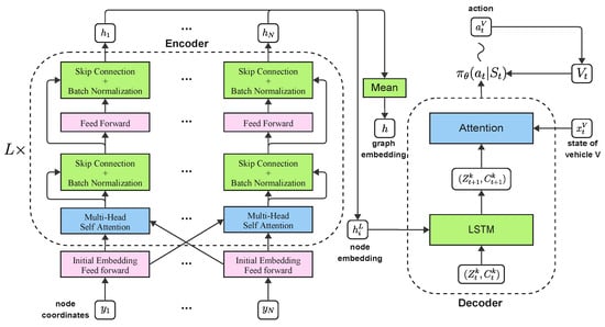
Figure 1.
An overview of the attention-encoder group-based LSTM-decoder model.
ENCODER. A multi-head attention-based encoder is deployed, which has been shown to be effective in embedding graphs for routing problems [10,25]. In the context of a given graph with nodes in and corresponding coordinates denoted as for each node , the process of embedding a fully connected graph begins with an initial transformation of node embeddings. The initial embeddings, represented as for all , involve learnable parameters and .
These initial node embeddings undergo L attention layers, where each layer, denoted as l, comprises two sublayers: a multi-head attention (MHA) layer and a fully connected feed-forward (FF) layer. The MHA layer takes input from the previous layer and facilitates message passing between nodes. For each input to the MHA layer, queries , keys , and values are computed by projecting the input using trainable parameters , and .
Compatibility between nodes i and j is determined based on the fully connected graph structure, expressed as , where represents the parameter size. The compatibility values are then used to compute attention weights, , using the softmax function. Messages received by node n are formed as convex combinations of messages from all nodes.
An MHA layer with head size M is employed to enhance the attention mechanism’s expressive power. Messages from each head are computed and combined for each node n. The output of the MHA sublayer, along with skip connections, undergoes batch normalization.
The resulting batch-normalized output is processed through a fully connected FF network with the ReLU activation function. Skip connections and batch normalization are applied again to the output of the FF layer, resulting in the final representation denoted as after l attention layers.
DECODER. The encoder outputs representing embeddings for each node in the graph are used to denote the graph encoding, represented as , which is defined as the mean of all node embeddings in the graph. For each group in the problem setting, where groups are defined by the number of trucks k, the LSTM is initialized consisting of a tuple for all .
To determine an action for a decision-maker, either a drone or the truck in group k at time t, the LSTM is provided with the embedding of the last node selected by the last decision-maker in the group, labeled as , where i corresponds to the node:
Moving to the decoder, the hidden state and cell state at time are subject to dropout with a probability of p:
To represent the state of the decision-maker at time t, binary values and are constructed to indicate whether the current decision-maker is in transit or not, and whether it has a load or not, respectively. The current battery level of a drone is normalized by the maximum battery level, , and is denoted as . Let vector denote the concatenation of , and .
The current state of the decision-maker , the embedding of the graph , and the hidden state of the LSTM are inputs to an attention mechanism, where the attention vector is computed using trainable parameters , and , and its elements are denoted as .
Subsequently, the attention vector undergoes softmax to generate probabilities for visiting the next node, as the following equation describes. Its value is set to zero if a node has been visited by any vehicle before:
4.2. The Training Algorithm
Efficient training of the attention-encoder group-based LSTM-decoder model involves exploring actions and receiving feedback as rewards. The model aims to determine the probability distribution, , that, given a graph, generates the sequence of nodes to be visited by both the drones and the trucks in the VRPD. The objective during training is to minimize the makespan C in Equation (4).
The training objective function, denoted as , is defined as:
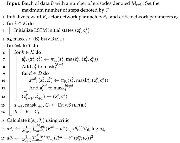
Here, serves as a baseline for variance reduction. A critic network estimates , while an actor-network is utilized to learn the policy . The gradients of the objective function, , are computed using the REINFORCE algorithm [31]. Algorithm 1 outlines the training process of actor and critic networks by sampling a batch of data from a predefined distribution and actions for all drones and trucks at each time step. Then, the final reward resulting at the end of the episode is used as an empirical mean to train both networks. To efficiently explore action spaces of drones and trucks, a masking scheme is employed that prevents some nodes from being visited based on the current state of the problem and the routing constraints, similar to existing literature [10,11]. In particular, a mask is applied during the action selection process, filtering out actions that violate constraints as shown in Algorithm 1.
| Algorithm 1: Rollout |
 |
5. Computational Studies
In this section, the proposed model is focused on through computational studies.
5.1. Training and Evaluation Configurations
Data Generation. To demonstrate the computational efficiency of the proposed approach, results are reported on the well-known benchmark dataset first proposed in [28]. In particular, ref. [28] randomly generated customer locations using a uniform distribution within the [1, 100] × [1, 100] area, while the depot location is generated with a uniform distribution within the [0, 1] × [0, 1] range, ensuring it always resides in a corner. Other studies have widely used the same benchmark dataset, including [9,30]. Throughout the experiments, it is assumed that the drone’s speed is double that of the truck, thus = 2, consistent with existing literature.
Gap. To evaluate the quality of solutions produced by different approaches to solve the VRPD, the GAP is measured and defined as:
where is the cost of a solution method for each instance i and is the cost of the best-performing solution method among all methods compared for instance i. In Table 1, Table 2 and Table 3, the average GAP for each setting of the problem as the mean of GAPs for 10 instances of the problem is reported.

Table 1.
The VRPD results with Infinite Flying Range of Drones. Averages of 10 problem instances. ‘Cost’ refers to the average cost value. ‘Gap’ is the mean relative difference to the cost of the best algorithm for each instance. ‘Time’ is the average solution time of the algorithm for a single instance.
Table 2.
The VRPD results with Limited Flying Range of Drones with . Averages of 10 problem instances.
Table 3.
The VRPD results with Limited Flying Range of Drones with . Averages of 10 problem instances.
Baselines. The efficiency of the proposed neural architecture is analyzed using [9] as a benchmark. In [9], the authors proposed the MILP formulation of the problem, solving the small instances exactly with and without lazy constraints, denoted as Solver and Solver Lazy, respectively in Table 1, Table 2 and Table 3. Beyond the exact method, the authors suggested a more practical strategy involving VNS and TS methods. This approach entails incorporating drones into delivery routes and a divide-and-conquer strategy. VNS is a method of exploring various possibilities by altering the neighbourhood structure, while TS is another approach that learns from previous solutions to avoid retracing steps. The results of VNS and TS-based heuristics are denoted as Heuristic in Table 1, Table 2 and Table 3. The computational time and costs for each instance of [9] have been kindly shared by the authors, where the best solution obtained by their heuristic in five runs and its corresponding computational time are reported.
Decoding Strategies. Three approaches were used to extract solutions from the trained model. The first method, referred to as “greedy”, involves consistently choosing nodes with the highest visitation probability at each time step. In the second method, “sampling”, multiple solutions are independently generated from the trained model with a sampling size of 4800. Subsequently, the solution with minimal cost among the samples is identified, and its results are reported. In the third method, “Ensemble”, multiple models saved throughout the training process are utilized. In particular, the models’ weights in the interval are selected with an increment of 100k. Solutions are sampled using a sample size of 4800 for each model, and the best results are reported.
Computational Resources and Hyperparameters. Computers with the following specifications were utilized: Intel Core i9 12900K and PCI-E 24576Mb Palit RTX 3090 GamingPro OC, GeForce RTX 3090 video card were used in two of the systems, while a Core i9 12900K with RTX 4090 24GB was employed on another computer for training. An Intel Core i9 12900K and PCI-E 24576Mb Palit RTX 3090 GamingPro OC computer were used to conduct testing and report the computational time.
The same hyperparameters as those in [13] were used to train the neural networks, including 256 as the hidden dimension for embedding, 0.0001 as the learning rate, and 1 million iterations for training.
5.2. Results on the VRPD with Unlimited Flying Range
- Single vehicle with two drones
- Two vehicles with one drone assigned to each vehicle
- Two vehicles with two drones assigned to each vehicle
For a small-scale problem with 8 nodes, the RL sampling model exhibits a 1.45% optimality gap. It demonstrates an almost 70-fold increase in speed within the first configuration. It outperforms all other methods in the second configuration and achieves a 2.14% optimality gap in the third configuration.
In a small-scale problem involving 10 nodes, the RL sampling model surpasses all alternative methods in the initial two configurations. The third configuration achieves a minimal 0.92% gap compared to exact methods. Since no results were reported for big-scale problems with 20 nodes, we only reported the RL model results.
The fast results from the RL sampling approach mostly come from its learned policies that use the problem’s structure effectively, such as grouping similar tasks. The proposed model adjusts when multiple drones are used by balancing their routes with the trucks. This adjustment shows in the nearly optimal solutions we see in the 8- and 10-node cases, indicating that our RL method can find efficient orders for dispatching without needing to check every possibility. However, we notice that as the problem size grows (for example, with 20 nodes), the quality of the solutions may drop a bit (1–2% higher gap) compared to smaller cases. This happens because tracking the coordination between drones and trucks gets more complicated, highlighting the balance between quick solutions and ensuring the best overall result.
In summary, findings show that the RL model can quickly create high-quality routes for different situations, offering clear advantages over traditional solvers in terms of speed. This speed can be crucial in real-world operations where route decisions need to change quickly.
5.3. Results on the VRPD with Limited Flying Range
The impact of restricted flying ranges was systematically explored by adjusting a crucial parameter denoted as . This parameter plays a vital role in defining the operational capabilities of the drone, specifically determining the maximum distance it can cover with a fully charged battery. The outcomes of these scenarios, detailed in Table 2 and Table 3, provide detailed insight into how the system performs under limited flying distances.
This specific variable is adopted based on empirical setups from [9]. In that study, was tested as a moderately restrictive constraint, limiting drones to 60% of the largest distance between any two nodes, while represented a more lenient scenario where drones could cover the entire maximum inter-node distance.
By using these two values, conducted experiments align with established benchmarks, allowing for direct comparisons with previous results. Additionally, these levels highlight how the proposed method adapts to different drone battery constraints: simulates stricter capacity limitations, whereas reflects drones capable of covering any route segment in a single trip. This setup helps evaluate how varying operational flexibility influences solution quality, route feasibility, and computational efficiency.
Scenario 1:
In the first scenario, where is set to 1, indicating the drone’s maximum flight distance aligns with the largest distance between nodes, the results are showcased in Table 2.
In smaller scenarios with 10 nodes, the Ensemble RL model outperforms Solver and Solver Lazy in terms of time and quality across all configurations. Compared to the Heuristic approach, Ensemble RL achieves a 1.04% gap in the first setup, showcasing nearly 60 times faster performance. The second configuration reveals a 2.03% gap with approximately a 16-fold speed boost, while the third setup shows a 2.3% gap with around 15 times faster speed.
In larger-scale problems involving 20 and 50 nodes, Ensemble RL demonstrates superior solution efficiency and time performance compared to the Heuristic method in the initial configuration. However, in the second and third configurations for , the gaps are 3.09% and 3.58%, respectively. For , Ensemble RL outperforms the Heuristic method in all configurations.
Scenario 2:
Transitioning to the second scenario is characterized by setting to 0.6, thus constricting the drone’s maximum flight distance to 60% of the largest distance between nodes. The results in Table 3 illuminate additional insights into the system’s adaptability and efficiency under different operational constraints.
Ensemble RL consistently outperformed Solver and Solver Lazy in our experiments with smaller instances across all configurations, demonstrating its reliable efficiency. Ensemble RL achieved a 1.28% gap compared to the Heuristic in the first setup. In the second configuration, Ensemble RL Sampling reduced the gap to 0.08%. In the third configuration, the Ensemble model showcased its ability to find a solution with only a 0.12% gap, and it did so with a significant approximately 10-fold increase in speed.
Shifting to more significant instances with 20 nodes, Ensemble RL sustained its superiority over the Heuristic in the first setup, excelling in speed and achieving the best solutions. This outstanding performance extended to instances with 50 nodes. Ensemble RL consistently outperformed the Heuristic in both the first and second setups, highlighting its scalability and effectiveness in handling more intricate problem scenarios. Considering the third scenario, RL Sampling outperformed the Heuristic with only a 0.18% optimality gap.
Under limited flight ranges (like when ), data shows that drones tend to stay closer to the trucks. This limits their ability to carry out independent missions. However, the RL-based approaches still keep competitive gaps of less than 2–3% in most cases. This means the learned policy successfully adapts to shorter drone routes. In practice, this suggests that logistics providers can effectively use drones even in challenging environments or when battery life is limited by taking advantage of adaptive route generation to ensure coverage. Additionally, the speed of RL-based sampling and Ensemble solutions is still a significant advantage. This speed is crucial in situations that require quick adjustments, such as when new customer orders come in or traffic conditions change.
5.4. Ablation Studies
To demonstrate the value of differentiating the group’s information in Equation (6), ablation studies are conducted comparing the performance of the RL greedy model with and without LSTM updates in Table 4, where the proposed group information updates are used as an input to the LSTM. As shown in the table, such a group differentiates and minimizes costs in all instances for various values of .
Table 4.
The ablation studies on comparing RL Greedy models with and without the LSTM group updates. The averages of 10 instances were reported for costs and gaps. The relative gap is computed for each instance with respect to the best model result among all benchmark models.
The ablation studies highlight the importance of updates at the group level for LSTM. When these updates are omitted, a consistent increase in the average cost is observed, typically between 2% and 3% for certain problem sizes. This shows that understanding interactions within the group, especially how each drone-truck pair works together, provides real benefits in performance. Therefore, the system’s ability to capture interactions between multiple agents is key to developing effective routing solutions.
5.5. Routing Solutions
Figure 2 demonstrates the results produced by the RL sampling approach on the first instance on a graph with 10 nodes from [28] with . As can be seen from the solutions, drones’ utilisation for customers is limited due to the small flying range corresponding to , where drones and trucks travel together to serve customers. In the case involving two trucks, Figure 2b,c show how the RL approach naturally solves the clustering problem of splitting the networks into two groups even though it has not been explicitly outlined in the MDP problem formulation. Instead, based on trial and error with the RL training, the proposed neural network architectures learn implicitly to cluster nodes to be served by two separate groups while ensuring the minimization of costs. Also, Figure 2 illustrates that increasing the number of drones doesn’t always improve the total serving time, given the small number of customers to serve and the small flying range of drones.
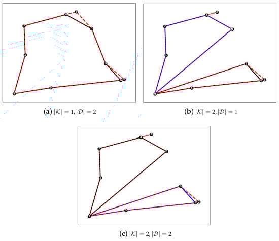
Figure 2.
Drones’ and trucks’ routes produced by the RL sampling approach with on a graph with 10 nodes. The solid lines in black and blue colors correspond to the first and second truck’s routes, and the dashed lines correspond to their assigned drones’ routes.
6. Conclusions
In this study, the main focus was on learning and coordinating multiple vehicles with multiple drones to optimize routing dynamics in scenarios involving both vehicles and drones. The exploration and evaluation, especially when testing the model on large and small instances using well-known benchmarks, provided valuable insights into its adaptability and efficiency.
The study, centred around various configurations manipulating factors like drone flight range, the number of vehicles, and drone allocations, consistently demonstrated the comparable performance of RL approaches with traditional methods. Notably, it demonstrated adaptability in scenarios with limited drone flight range, delivering solutions that balance quality and computational speed.
The findings reinforce that the RL model holds significant promise for addressing challenges and optimizing efficiency in drone-assisted vehicle routing. Further exploration of this model, particularly in scenarios involving an increased number of vehicles and drones, presents exciting opportunities to enhance its optimality and robustness in real-world logistics applications.
Additionally, exploring scenarios with an increased number of nodes could provide valuable insights and contribute to the continued advancement of this research field. In conclusion, this research suggests that RL-based models are valuable for planning routes involving vehicles and drones. Exploring its capabilities more thoroughly, the promising potential is seen to improve how deliveries are managed in the future.
Despite these promising directions, the current study has certain limitations that warrant further investigation. First, complex recharging or maintenance schedules for drones are not explicitly modeled, which may limit the applicability of the approach in extended delivery routes or highly variable environments. Second, although strong adaptability is demonstrated by the proposed model in benchmark settings, the robustness would be better validated through additional testing with real-world datasets and unpredictable factors (e.g., weather conditions and traffic disruptions). Finally, while multiple drones and vehicles are considered, exploring larger-scale deployments and more intricate constraints (e.g., multi-objective objectives balancing cost, time, and environmental impact) could uncover new challenges and optimization opportunities. Future work could address these aspects by integrating dynamic recharging strategies, employing real-time data streams for adaptive routing, and evaluating the performance across a broader range of industrial and urban scenarios. It is believed that the proposed reinforcement learning framework can evolve into a fully operational tool for last-mile logistics and beyond by being implemented.
Author Contributions
Conceptualization, B.D. and M.M.; methodology, A.B.; software, B.D.; validation, M.M. and A.B.; formal analysis, M.M.; investigation, A.B.; resources, A.B.; data curation, B.D.; writing—original draft preparation, B.D.; writing—review and editing, A.B.; visualization, M.M.; supervision, A.B.; project administration, M.M.; funding acquisition, A.B. All authors have read and agreed to the published version of the manuscript.
Funding
This research was funded by the Ministry of Science and Higher Education of the Republic of Kazakhstan, IRN AP19575607.
Institutional Review Board Statement
Not applicable.
Informed Consent Statement
Not applicable.
Data Availability Statement
Data is available upon a request from the authors.
Conflicts of Interest
The funders had no role in the design of the study; in the collection, analyses, or interpretation of data; in the writing of the manuscript; or in the decision to publish the results.
Appendix A
We consider a limited set K of vehicles. Furthermore, each vehicle holds an equal number of drones assigned to it. Each drone may travel a maximum range of E distance units per operation, where a drone-operation is characterized by a triple as follows: the drone is launched from a vehicle at a node , delivers a parcel to , and is retrieved by the vehicle from which it was launched at node ( and ).
We use the following decision variables for modeling the VRPD:
- : – Binary variables that state whether edge belongs to the route of vehicle k.
- : – Binary variables that specify whether drone delivery is performed by a drone associated with vehicle k.
- : – Binary variables that indicate whether node i is served before (but not necessarily consecutive to) node j in the route of vehicle k.
- : – Integer variables with a lower bound of 0 that state the position of node i in the route of vehicle k, if customer i is served by vehicle k.
- : – Binary variables that specify whether the drone delivery is performed by a drone associated with vehicle k and node a precedes node i while node e follows node j in the route of vehicle k.
- : – Continuous variables with a lower bound of 0 that indicate the earliest time at which customer i is served by either the vehicle k or a drone associated with vehicle k. If i is used as a retrieval node, is the earliest time at which both the (latest) drone and the vehicle have arrived at node i.
The MILP formulation of the VRPD is given in (A1)–(A19), where (A1) is the objective function and the constraints are given by (A2)–(A19):
The constraints (A3)–(A19) ensure the flow preservation, synchronization between vehicles and drones, and maximum range of drone operations, as well as satisfying other operational restrictions. The objective function minimizes the arrival time , which represents the time when the last vehicle or its associated drones return to the depot.
References
- Deloison, T.; Hannon, E.; Huber, A.; Heid, B.; Klink, C.; Sahay, R.; Wolff, C. The future of the last-mile ecosystem. In Proceedings of the World Economic Forum, Davos, Switzerland, 21–24 January 2020; Volume 1, pp. 1–28. [Google Scholar]
- Mahadevan, P. The military utility of drones. CSS Anal. Secur. Policy 2010, 78. [Google Scholar]
- Restas, A. Drone applications for supporting disaster management. World J. Eng. Technol. 2015, 3, 316. [Google Scholar] [CrossRef]
- Macrina, G.; Pugliese, L.D.P.; Guerriero, F.; Laporte, G. Drone-aided routing: A literature review. Transp. Res. Part C Emerg. Technol. 2020, 120, 102762. [Google Scholar] [CrossRef]
- Borghetti, F.; Caballini, C.; Carboni, A.; Grossato, G.; Maja, R.; Barabino, B. The use of drones for last-mile delivery: A numerical case study in Milan, Italy. Sustainability 2022, 14, 1766. [Google Scholar] [CrossRef]
- Wang, X.; Poikonen, S.; Golden, B. The vehicle routing problem with drones: Several worst-case results. Optim. Lett. 2017, 11, 679–697. [Google Scholar] [CrossRef]
- Wang, Z.; Sheu, J.B. Vehicle routing problem with drones. Transp. Res. Part B Methodol. 2019, 122, 350–364. [Google Scholar] [CrossRef]
- Poikonen, S.; Wang, X.; Golden, B. The vehicle routing problem with drones: Extended models and connections. Networks 2017, 70, 34–43. [Google Scholar] [CrossRef]
- Schermer, D.; Moeini, M.; Wendt, O. A hybrid VNS/Tabu search algorithm for solving the vehicle routing problem with drones and en route operations. Comput. Oper. Res. 2019, 109, 134–158. [Google Scholar] [CrossRef]
- Kool, W.; van Hoof, H.; Welling, M. Attention, Learn to Solve Routing Problems! arXiv 2019, arXiv:1803.08475. [Google Scholar]
- Nazari, M.; Oroojlooy, A.; Snyder, L.; Takác, M. Reinforcement learning for solving the vehicle routing problem. In Proceedings of the Advances in Neural Information Processing Systems 31 (NeurIPS 2018), Montréal, QC, Canada, 3–5 December 2018. [Google Scholar]
- Bogyrbayeva, A.; Meraliyev, M.; Mustakhov, T.; Dauletbayev, B. Machine Learning to Solve Vehicle Routing Problems: A Survey. IEEE Trans. Intell. Transp. Syst. 2024, 25, 4754–4772. [Google Scholar] [CrossRef]
- Bogyrbayeva, A.; Yoon, T.; Ko, H.; Lim, S.; Yun, H.; Kwon, C. A deep reinforcement learning approach for solving the traveling salesman problem with drone. Transp. Res. Part C Emerg. Technol. 2023, 148, 103981. [Google Scholar] [CrossRef]
- Schermer, D.; Moeini, M.; Wendt, O. Algorithms for solving the vehicle routing problem with drones. In Proceedings of the Intelligent Information and Database Systems: 10th Asian Conference, ACIIDS 2018, Dong Hoi City, Vietnam, 19–21 March 2018; Proceedings, Part I 10. Springer: Berlin/Heidelberg, Germany, 2018; pp. 352–361. [Google Scholar]
- Schermer, D.; Moeini, M.; Wendt, O. A matheuristic for the vehicle routing problem with drones and its variants. Transp. Res. Part C Emerg. Technol. 2019, 106, 166–204. [Google Scholar] [CrossRef]
- Wu, G.; Fan, M.; Shi, J.; Feng, Y. Reinforcement learning based truck-and-drone coordinated delivery. IEEE Trans. Artif. Intell. 2021, 4, 754–763. [Google Scholar] [CrossRef]
- Chiaraviglio, L.; D’andreagiovanni, F.; Choo, R.; Cuomo, F.; Colonnese, S. Joint optimization of area throughput and grid-connected microgeneration in UAV-based mobile networks. IEEE Access 2019, 7, 69545–69558. [Google Scholar] [CrossRef]
- Otto, A.; Agatz, N.; Campbell, J.; Golden, B.; Pesch, E. Optimization approaches for civil applications of unmanned aerial vehicles (UAVs) or aerial drones: A survey. Networks 2018, 72, 411–458. [Google Scholar] [CrossRef]
- Shi, Y.; Lin, Y.; Li, B.; Li, R.Y.M. A bi-objective optimization model for the medical supplies’ simultaneous pickup and delivery with drones. Comput. Ind. Eng. 2022, 171, 108389. [Google Scholar] [CrossRef]
- Trotta, A.; Andreagiovanni, F.D.; Di Felice, M.; Natalizio, E.; Chowdhury, K.R. When UAVs ride a bus: Towards energy-efficient city-scale video surveillance. In Proceedings of the IEEE Infocom 2018-IEEE Conference on Computer Communications, Honolulu, HI, USA, 16–19 April 2018; pp. 1043–1051. [Google Scholar]
- Mazyavkina, N.; Sviridov, S.; Ivanov, S.; Burnaev, E. Reinforcement learning for combinatorial optimization: A survey. Comput. Oper. Res. 2021, 134, 105400. [Google Scholar] [CrossRef]
- Bello, I.; Pham, H.; Le, Q.V.; Norouzi, M.; Bengio, S. Neural combinatorial optimization with reinforcement learning. arXiv 2016, arXiv:1611.09940. [Google Scholar]
- Vinyals, O.; Fortunato, M.; Jaitly, N. Pointer networks. In Proceedings of the Advances in Neural Information Processing Systems 28 (NIPS 2015), Montreal, QC, Canada, 7–12 December 2015. [Google Scholar]
- Khalil, E.; Dai, H.; Zhang, Y.; Dilkina, B.; Song, L. Learning combinatorial optimization algorithms over graphs. In Proceedings of the Advances in Neural Information Processing Systems 30 (NIPS 2017), Long Beach, CA, USA, 4–9 December 2017. [Google Scholar]
- Kwon, Y.D.; Choo, J.; Kim, B.; Yoon, I.; Gwon, Y.; Min, S. Pomo: Policy optimization with multiple optima for reinforcement learning. Adv. Neural Inf. Process. Syst. 2020, 33, 21188–21198. [Google Scholar]
- Kim, M.; Park, J. Learning Collaborative Policies to Solve NP-hard Routing Problems. In Proceedings of the Advances in Neural Information Processing Systems 34 (NIPS 2021), Online, 6–14 December 2021. [Google Scholar]
- Ma, Y.; Li, J.; Cao, Z.; Song, W.; Zhang, L.; Chen, Z.; Tang, J. Learning to Iteratively Solve Routing Problems with Dual-Aspect Collaborative Transformer. In Proceedings of the Advances in Neural Information Processing Systems 34 (NIPS 2021), Online, 6–14 December 2021. [Google Scholar]
- Agatz, N.; Bouman, P.; Schmidt, M. Optimization approaches for the traveling salesman problem with drone. Transp. Sci. 2018, 52, 965–981. [Google Scholar] [CrossRef]
- Schermer, D.; Moeini, M.; Wendt, O. A Variable Neighborhood Search Algorithm for Solving the Vehicle Routing Problem with Drones; Technacal Report; Technische Universität Kaiserslautern: Kaiserslautern, Germany, 2018. [Google Scholar]
- Bogyrbayeva, A.; Jang, S.; Shah, A.; Jang, Y.J.; Kwon, C. A reinforcement learning approach for rebalancing electric vehicle sharing systems. IEEE Trans. Intell. Transp. Syst. 2021, 23, 8704–8714. [Google Scholar] [CrossRef]
- Williams, R.J. Simple statistical gradient-following algorithms for connectionist reinforcement learning. Mach. Learn. 1992, 8, 229–256. [Google Scholar] [CrossRef]
Disclaimer/Publisher’s Note: The statements, opinions and data contained in all publications are solely those of the individual author(s) and contributor(s) and not of MDPI and/or the editor(s). MDPI and/or the editor(s) disclaim responsibility for any injury to people or property resulting from any ideas, methods, instructions or products referred to in the content. |
© 2025 by the authors. Licensee MDPI, Basel, Switzerland. This article is an open access article distributed under the terms and conditions of the Creative Commons Attribution (CC BY) license (https://creativecommons.org/licenses/by/4.0/).