Research on Price Prediction of Construction Materials Based on VMD-SSA-LSTM

Abstract

This study proposes a novel hybrid model, VMD-SSA-LSTM, aimed at enhancing the accuracy of construction material price (CMP) predictions. The model integrates Variational Mode Decomposition (VMD) for signal decomposition, the Sparrow Search Algorithm (SSA) for parameter optimization, and Long Short-Term Memory (LSTM) networks for predictive modeling. Historical CMP data are first decomposed into intrinsic components using VMD, followed by the SSA-based optimization of the LSTM parameters. These components are then input into the LSTM network for final predictions, which are aggregated to produce the CMP forecast. Experimental results using rebar price data from Hengyang City demonstrate that the VMD-SSA-LSTM model outperforms the backpropagation (BP) neural network, LSTM, and VMD-LSTM models in terms of prediction accuracy. The proposed method provides highly valuable tools for construction cost management, significantly enhancing the reliability of budget planning and risk mitigation decisions, and has significant practical implications for engineering cost risk management.

1. Introduction

1.1. Background and Significance of the Research

In construction projects, material costs account for a substantial proportion of the total budget, and fluctuations in material prices significantly impact cost control and profitability. For instance, previous studies have shown that materials constitute 25–40% of the total cost of a typical steel frame structure [1]. Enhancing the accuracy of material price prediction can improve the precision of cost estimates, as approximately one-fourth of the total cost of construction projects is attributed to material costs. However, estimating material costs remains a challenging task due to price fluctuations during the construction period. Consequently, the accurate forecasting of material prices is essential for effective construction cost risk management [2].

The key aspects of this necessity include the following:

• Reducing cost uncertainties and improving budget accuracy: accurate price forecasting mitigates the impact of material price fluctuations on budgeting, thereby enhancing the reliability of financial planning for projects.
• Supporting decision-making and optimizing risk mitigation strategies: reliable predictions form a strong basis for implementing risk management measures, such as hedging and fixed-price contracts.
• Enhancing risk management capabilities and minimizing schedule delays and contractual disputes: fluctuations in material prices frequently lead to project schedule adjustments and contractual conflicts, which can be mitigated through accurate price forecasting.
• Strengthening corporate competitiveness: the ability to accurately predict material prices constitutes a strategic advantage, enabling firms to submit more competitive bids in tendering processes.

Construction costs are a primary concern for project managers due to significant price volatility and frequent design changes during the construction process. In the face of such uncertainty, reliable cost forecasts serve as crucial decision-making tools for all stakeholders [3]. By employing advanced scientific methods for material price forecasting, companies can better control costs, gain a competitive edge, and ultimately enhance overall project management efficiency [4].

Material price fluctuations are a major source of deviation from initial cost estimates. These fluctuations are driven by factors including raw material prices, energy costs, and market conditions, making predictions challenging due to the unpredictable nature of these influences [5,6,7]. Reliable CMP predictions empower companies to anticipate market trends, reduce investment risks, and allocate resources more efficiently. This not only strengthens economic stability but also enhances the operational efficiency of construction projects. For contractors, a thorough understanding of market conditions and the accurate forecasting of future CMP trends are indispensable for making well-informed decisions during the bidding and planning phases. Such informed decision-making directly affects key aspects of project management, including scheduling, quality control, and cost management [8]. Therefore, having a reliable and accurate method for predicting material prices in the early stages of construction is crucial. This research aims to propose a novel approach to material price prediction.

As previously mentioned, material costs significantly impact the overall project budget. Inaccurate predictions of material prices can lead to cost overruns. Therefore, it is essential to develop a reliable and precise method for forecasting material costs. Several studies have focused on predicting the Construction Cost Index [9,10,11] (CCI), which includes all cost components such as material, labor, and machinery costs. However, to improve accuracy, it is more effective to analyze material costs separately. The following section reviews previous research on predicting material prices using various methods. These studies commonly employed regression analysis [12], time series methods, machine learning, or combinations of these techniques [13]. However, regression and statistical analyses are limited in terms of the number of influencing factors they can consider, and they cannot measure the combined effects of these factors. In expert systems, personal biases may influence the rules derived from domain experts. Artificial intelligence techniques, including neural networks, machine learning, and time series analysis, are particularly well-suited for material price prediction due to their dynamic learning mechanisms and strong pattern recognition capabilities.

1.2. Current Status of Research

Studies have shown that various methods, including time series analysis, support vector machine regression (SVR), gray prediction (GM), system dynamics (SD), and neural network models, are widely used for forecasting construction material prices. In response to price fluctuations, researchers and industry experts have developed a range of forecasting approaches, such as statistical models (e.g., ARIMA), machine learning techniques (e.g., Long Short-Term Memory [14] (LSTM)), and hybrid methods. Each of these methods offers distinct advantages and limitations, making them suitable for different types of data and forecasting objectives.

BP neural networks (backpropagation neural networks) are widely used in nonlinear prediction tasks due to their strong nonlinear fitting capability. For instance, Jiang J et al. [15] applied BP neural network to establish a price prediction model for construction materials to realize the prediction of CMP trends. The prediction results are basically consistent with the actual prices. Ouyang H et al. [16] proposed taking the historical price information of materials as a sample and constructing a model with the help of BP neural network to predict the future trend of CMP. However, BP networks are prone to falling into local optima, require long training times, and demand large amounts of data. Grey model (GM (1,1)) prediction is well suited to handling small sample datasets and can even make predictions when data are limited. For example, Wang Y [17] predicted the steel prices from June to December 2012 by establishing a GM (1,1) and taking the market steel price data of Zhengzhou city from January to July 2012 as an example. However, GMs (1,1) are highly dependent on the available data, and their prediction accuracy is often limited. ARIMA (autoregressive integrated moving average) is a well-established time series forecasting method that models data based on autocorrelation. It is widely used for short-term predictions, particularly for stationary time series. While ARIMA is simple and easy to understand, it has limitations in handling nonlinear relationships and long-term dependencies. For instance, Suad H et al. [18] employed ARIMA and multiple regression models to predict CMP. Wang J et al. [19] used the time series method to forecast the short-term price using the historical cost information of steel prices, and based on the ARIMA model, they predicted the steel prices over the next three months and achieved good prediction results. Wang J et al. [20] utilized the time series method to predict and analyze the historical price data of construction materials accumulated in a construction cost information database. Nguyen V H et al. [21] used the autoregressive integrated moving average (ARIMA) model to predict the sales data of dehumidifiers and heat pumps in the projects extracted from the website. Mir Mostafa et al. [12] utilized artificial neural network (ANNs) to quantify uncertainty through generating prediction intervals, thereby achieving the purpose of predicting the price range of construction materials. In contrast to ARIMA, artificial neural networks (ANNs) are inspired by the human brain’s structure and are capable of modeling complex nonlinear patterns through dynamic learning. However, ANNs are prone to overfitting and require large datasets and significant computational resources. More recently, Long Short-Term Memory (LSTM) networks, using a deep learning technique, have demonstrated superior performance in time series forecasting. Peng Y et al. [22], by combining the characteristics of LSTM (Long Short-Term Memory) recurrent neural networks and those of the stock market, preprocessed data through interpolation, wavelet noise reduction, and normalization. Subsequently, they pushed the data into different models, namely the LSTM network model with the same number of hidden neurons in different LSTM layers and the LSTM network model with different numbers of hidden neurons in the same LSTM layer, to perform stock price prediction and analysis. Huang C et al. [23] used more than 7000 pieces of SSE Composite Index data and the LSTM neural network model to predict and analyze the SSE Composite Index. Fang J et al. [24] found that traditional statistics- and econometrics-based time series forecasting models have certain limitations in terms of long-term dependence, constructed a multilayer LSTM network price forecasting model, and used China’s soybean futures price data from 2007–2019 to carry out empirical research, and the results showed that the LSTM network model performs well in price forecasting. Despite its advantages in capturing complex nonlinear relationships, LSTM still faces challenges in handling noisy data and optimizing model parameters.

Existing research highlights significant advancements in addressing fluctuations in construction material prices through the development of various forecasting methods. Ranging from traditional statistical models to advanced AI-based algorithms, these approaches have aimed to enhance forecasting accuracy. However, each method exhibits inherent limitations. Traditional time series models, such as ARIMA, rely on assumptions of linearity and stationarity, rendering them less effective at capturing complex nonlinear and non-stationary features. Conversely, artificial neural networks (e.g., LSTM) demonstrate strong capabilities in modeling complex nonlinear relationships but face challenges in handling noisy data and optimizing parameters. To address these limitations, hybrid models have emerged as a prominent research focus in recent years. For instance, Tu, J. et al. [25] optimized the concrete strength prediction model by integrating a genetic algorithm (GA) with a BP neural network. The GA was employed to optimize the neural network’s weights and biases, enhancing both prediction accuracy and stability. The study’s results demonstrated that the GA-BP neural network model effectively predicted the strength of recycled aggregate thermal insulation concrete, exhibiting high accuracy and practicality. Luo Z et al. [26] utilized historical price data for construction materials to develop a grey neural network (PGNN) model by combining the GM (1,1) with a BP neural network in MATLAB. This approach significantly improved forecasting stability by leveraging the complementary strengths of the two methods. Similarly, Shiha A et al. [27] employed a genetic algorithm to optimize a neural network model using specialized software, thereby enhancing prediction accuracy. Tang B et al. [28] proposed a forecasting approach based on least-squares support vector machine, optimized with improved particle swarm optimization (IPSO). By rigorously training and testing the LSSVM model, they achieved substantial improvements in predicting future material prices.

In the aforementioned studies, most authors utilized mathematical statistical methods and neural network approaches to construct models for CMP prediction. It is evident that the prediction accuracy of a single model can achieve allow us to good results, but there is still room for further improvement. To enhance the predictive accuracy of the models, many authors employ optimization algorithms for model optimization. Experimental results indicate that the predictive accuracy of the optimized models has significantly improved. Recent advancements in hybrid modeling have shown promise in enhancing prediction accuracy by addressing the limitations of individual models. While neural network-based approaches, such as Long Short-Term Memory (LSTM) networks, capture nonlinear dependencies effectively, their predictive performance can degrade in noisy and non-stationary environments.

Below is a table comparing different construction material price forecasting methods, as shown in Table 1.

As shown in the table above, which compares the state of the art in research and research methods, traditional statistical techniques like ARIMA and GM (1,1) are suitable for short-term, linear, or small-sample data but struggle with nonlinear problems. On the other hand, neural networks and machine learning methods excel at capturing complex nonlinear patterns but are sensitive to noise and prone to overfitting, making them dependent on robust datasets and optimization techniques. Hybrid methods combine multiple techniques to enhance accuracy and robustness, e.g., LSTM combined with preprocessing or optimization algorithms. Furthermore, optimization algorithms (e.g., SSA, PSO) and signal decomposition techniques (e.g., VMD) improve model performance by refining parameter tuning and reducing noise.

1.3. Innovation Points

Neural networks, such as BP and LSTM, address some of these limitations by capturing nonlinear relationships, yet their predictive accuracy can be further enhanced through data preprocessing and parameter optimization. Recent research highlights the strong potential of hybrid models (e.g., VMD-SSA-LSTM) for forecasting complex, non-stationary data like construction material prices, offering the industry more accurate and reliable predictive tools. Variational Modal Decomposition [29] (VMD) is a powerful tool used for signal decomposition, effectively separating noisy components from meaningful data. The Sparrow Search Algorithm [30] (SSA) is a bio-inspired optimization technique that fine-tunes model parameters, reducing overfitting and improving convergence. When combined with LSTM, these methods create a robust framework capable of handling complex, non-stationary time series data. In this paper, examples are presented to validate the prediction accuracy and effectiveness of the VMD-SSA-LSTM model. The experimental results show that the VMD-SSA-LSTM model proposed in this paper significantly outperforms the traditional BP, LSTM, and VMD-LSTM models in terms of prediction accuracy. Especially in the prediction of highly volatile data, the model demonstrates stronger stability and reliability, providing an effective tool for engineering cost management.

Table 1. Comparison table of different construction material price forecasting methods.

Category	Method	Characteristics	Limitations	Submitter
Statistical models	ARIMA	Time series analysis, suitable for linear and stationary data	Assumes linearity and stationarity, cannot handle nonlinearity	Suad H et al. [18]; Wang J et al. [19,20]
	GM (1,1)	Grey forecasting, analyzes small sample data	Sensitive to input data quality, poor for long-term forecasting	Wang Y [17]
Machine learning	Support Vector Machine (SVM)	Regression modeling for small to medium datasets	Sensitive to parameter tuning, requires thorough preprocessing	Tang B et al. [28]
	Artificial Neural Networks (ANN)	Mimics brain structure, strong nonlinear modeling	Prone to overfitting, demands large datasets and computational resources	Jiang J et al. [15]; Mir Mostafa et al. [12]
	Long Short-Term Memory (LSTM)	A type of recurrent neural network, captures long-term dependencies	Sensitive to noise and non-stationary data, complex optimization	Huang C et al. [23]; Fang J et al. [24];
Hybrid approaches	GM (1,1) + BP Neural Network	Combines grey forecasting and neural networks for improved accuracy	Higher computational complexity	Luo Z et al. [26]
	LSTM + Data Preprocessing	Combines interpolation, noise reduction, normalization with LSTM	Complex preprocessing, high implementation requirements	Peng Y et al. [22]
	LSTM +VMD	Signal decomposition (VMD) + LSTM	High computational cost, complex implementation and validation	Wang J et al. [31]
	LSTM + SSA	Optimization (SSA) + LSTM	High computational cost, complex implementation and validation	Zhao J et al. [32]
Optimization algorithms	genetic algorithm (GA) or particle swarm optimization (PSO)	Optimizes neural network parameters	Prone to local optima, sensitive to initial parameters	Shiha A et al. [27]; Tu J et al. [25]; Tang B et al. [28]

Table 1. Comparison table of different construction material price forecasting methods.

Category	Method	Characteristics	Limitations	Submitter
Statistical models	ARIMA	Time series analysis, suitable for linear and stationary data	Assumes linearity and stationarity, cannot handle nonlinearity	Suad H et al. [18]; Wang J et al. [19,20]
	GM (1,1)	Grey forecasting, analyzes small sample data	Sensitive to input data quality, poor for long-term forecasting	Wang Y [17]
Machine learning	Support Vector Machine (SVM)	Regression modeling for small to medium datasets	Sensitive to parameter tuning, requires thorough preprocessing	Tang B et al. [28]
	Artificial Neural Networks (ANN)	Mimics brain structure, strong nonlinear modeling	Prone to overfitting, demands large datasets and computational resources	Jiang J et al. [15]; Mir Mostafa et al. [12]
	Long Short-Term Memory (LSTM)	A type of recurrent neural network, captures long-term dependencies	Sensitive to noise and non-stationary data, complex optimization	Huang C et al. [23]; Fang J et al. [24];
Hybrid approaches	GM (1,1) + BP Neural Network	Combines grey forecasting and neural networks for improved accuracy	Higher computational complexity	Luo Z et al. [26]
	LSTM + Data Preprocessing	Combines interpolation, noise reduction, normalization with LSTM	Complex preprocessing, high implementation requirements	Peng Y et al. [22]
	LSTM +VMD	Signal decomposition (VMD) + LSTM	High computational cost, complex implementation and validation	Wang J et al. [31]
	LSTM + SSA	Optimization (SSA) + LSTM	High computational cost, complex implementation and validation	Zhao J et al. [32]
Optimization algorithms	genetic algorithm (GA) or particle swarm optimization (PSO)	Optimizes neural network parameters	Prone to local optima, sensitive to initial parameters	Shiha A et al. [27]; Tu J et al. [25]; Tang B et al. [28]

2. Methodology

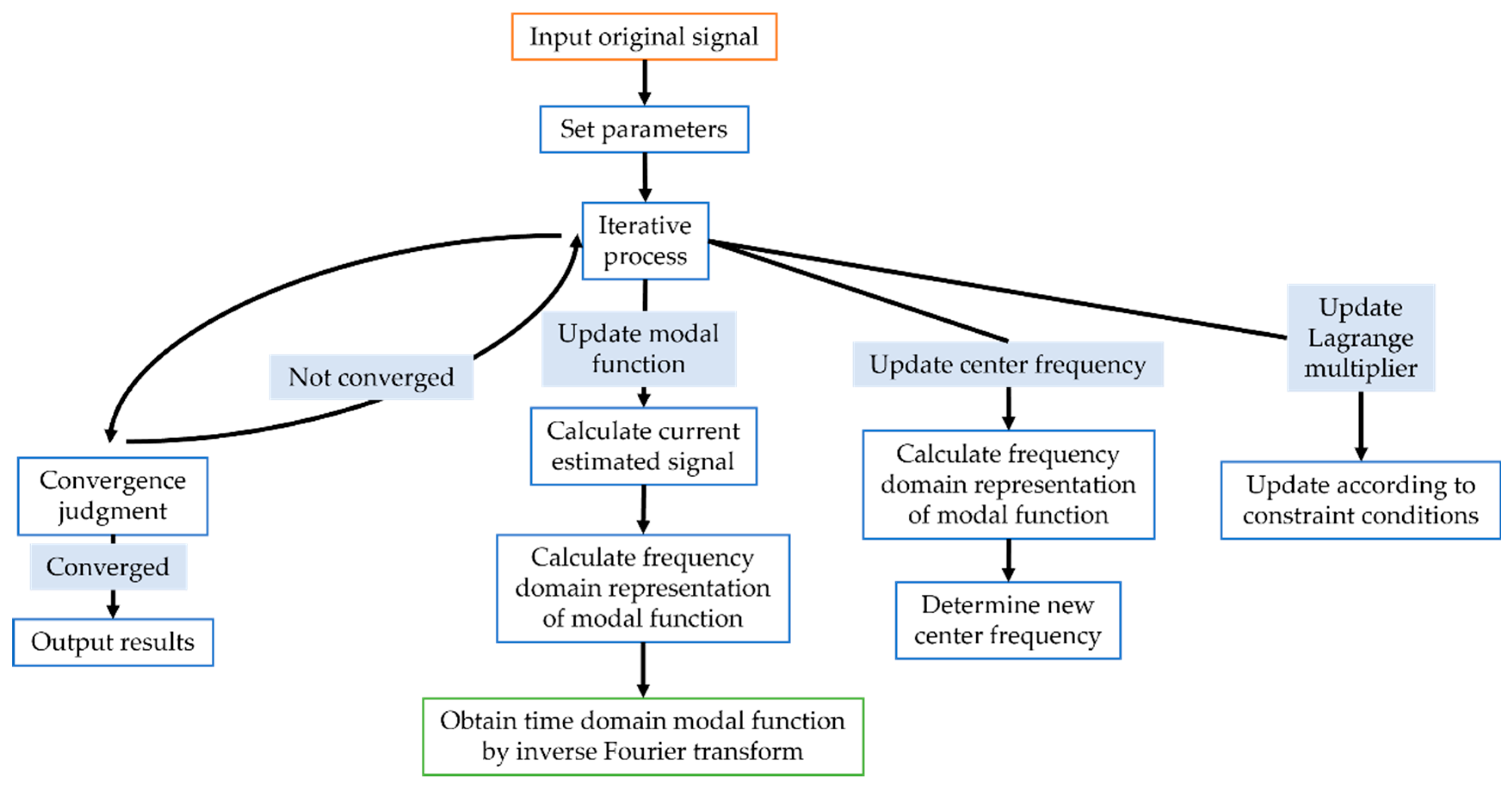
2.1. Variational Mode Decomposition (VMD)

Wang et al. [31] applied Variational Mode Decomposition (VMD) and integrated it with LSTM to develop a novel wind speed prediction model, VMD-LSTM. The proposed model significantly improved both the prediction accuracy and performance. VMD is a powerful signal processing tool that decomposes a complex signal into multiple Intrinsic Mode Function (IMF) components with different center frequencies. Figure 1 is a detailed flowchart of the VMD.

The center frequency and bandwidth of each mode function are determined adaptively without the need to pre-set the basis functions, making VMD suitable for processing non-stationary signals and signals with complex frequency characteristics. VMD uses the alternating-direction multiplier method (ADMM) to decompose $f(t)$ into K subsequences. The specific steps and formulas are given in Equations (1)–(4).

Step 1: for each $u_k$, the associated analytic signal is computed using the Hilbert transform and the spectrum is constructed.

$${\widehat{u}}_k^{n+1}(\omega )={\displaystyle \frac{\widehat{f}(\omega )-{\displaystyle {\sum }_{i\ne k}{\widehat{u}}_i^{n+1}(\omega )}+{\widehat{\lambda }}^n(\omega )/2}{1+2\alpha {(\omega +{\omega }_k^n)}^2}}$$

(1)

Step 2: the modal spectrum is shifted to the baseband using the respective estimated center frequencies, which are calculated as follows

$${\omega }_k={\displaystyle \frac{{{\displaystyle {\int }_0^{\infty }\omega \left|{\widehat{u}}_k(\omega )\right|}}^{2}d\omega }{{{\displaystyle {\int }_0^{\infty }\left|{\widehat{u}}_k(\omega )\right|}}^{2}d\omega }}$$

(2)

Step 3: Introducing a quadratic penalty term and the Lagrange multiplier $\lambda$ makes the problem unconstrained; the bandwidth is estimated by the Gaussian smoothness of the demodulated signal, i.e., the $L^2$-parameter of the gradient. The Lagrange multiplier $\lambda$ formula is updated as follows

$${\lambda }^{n+1}={\lambda }^n+\tau (f-{\displaystyle \sum _{k=1}^K{u}_k^{n+1}})$$

(3)

Step 4: The resulting constrained variational problem is as follows

$$\left\{\begin{array}{l}\underset{\left\{u_k\right\},\left\{{\omega }_k\right\}}{{\displaystyle \min }}\left\{{\displaystyle \sum _{k=1}^K{‖{\partial }_t\left[(\delta (t)+\frac{j}{\pi t})\ast u_k(t)\right]e^{-j{\omega }_{k}t}‖}_2^2}\right\}\\ S,T,{\displaystyle \sum _{k=1}^K{u}_k=f}\end{array}\right.$$

(4)

where $\widehat{f}(\omega )$ is the $f(t)$ Fourier transform of the input signal and ${\widehat{u}}_i^{n+1}$ and ${\widehat{\lambda }}^n(\omega )$ are the Fourier transforms of the updated modal function and the Lagrange multiplier, respectively.$\ast$ denotes the convolution operation, ${\partial }_t$ is the derivative with respect to time, $\delta (t)$ is the Dirac function, $j$ is the imaginary unit, ${‖·‖}_2^2$ is the $L^2$-parameter, and is $u_k$ the modal function. The solution is finally performed using the alternating-direction multiplier method (ADMM).

2.2. Optimization Algorithm

Zhao et al. [32] proposed a method to improve prediction accuracy and address the challenges associated with random selection and the difficulty of choosing parameters for LSTM networks. They employed the Sparrow Search Algorithm (SSA) algorithm to optimize model parameters and demonstrated that this approach significantly enhances prediction accuracy. This study employs the SSA to optimize three parameters of the LSTM model, with the aim of enhancing both prediction accuracy and model stability. The SSA is a novel swarm intelligence optimization technique inspired by the natural foraging and anti-predatory behaviors of sparrows. Figure 2 presents a detailed flowchart outlining its steps and mechanisms.

The SSA optimization process is specifically as follows:

• Producer update: A portion of sparrows (usually a certain percentage of the population, such as 10–20%) are considered producers. They are responsible for finding better food resources (i.e., better solutions) in the search space. The position update formula for producers is as follows:

$$X_{i,j}^{t+1}=\left\{\begin{array}{cc}{X}_{i,j}^t·\exp (-{\displaystyle \frac{i}{\alpha ·T}})& R_2<S_T\\ X_{i,j}^t+Q·L& R_2\ge S_T\end{array}\right.$$

(5)

where $X_{i,j}^t$ represents the position in the $j$-th dimension of the $i$-th sparrow in the $t$-th generation. $\alpha$ is a random number within the interval $\left(0,1\right]$, usually around 0.5, $T$ is the maximum number of iterations for the algorithm. $R_2\in \left[0,1\right]$ and $S_T\in \left[0.5,1\right]$ represent the range of the warning values and the range of the safe values, respectively. $Q$ is a random number that follows a standard normal distribution. $L$ is a matrix filled with ones. This formula allows producer sparrows to explore in the search space. As the number of iterations increases, the exploration range gradually decreases.

2.

Consumer update: The remaining sparrows are considered consumers. They follow the producers to find food resources. Consumer sparrows update their positions by randomly selecting a producer and approaching it. At the same time, they are also influenced by random factors to increase search diversity. The position update formula for consumers is as follows:

$$X_{i,j}^{t+1}=\left\{\begin{array}{cc}Q·\exp ({\displaystyle \frac{X_{w}os{t}^t-X_{i,j}^t}{i^2}})& i>{\displaystyle \frac{n}{2}}\\ X_p^{t+1}+\left|X_{i,j}^t-X_p^{t+1}\right|·A^{+}·L& i\le {\displaystyle \frac{n}{2}}\end{array}\right.$$

(6)

where $X_{w}os{t}^t$ represents the position of the global worst sparrow in the t-th generation, $X_p^{t+1}$ denotes the best position occupied by consumers in generation $t+1$, $n$ is the total number of sparrow populations, $A$ is a $1\times d$ matrix, and each element in the $A^{+}$ matrix is randomly assigned a value of 1 or −1.

3.

Scout update: In the sparrow population, there will also be some sparrows acting as scouts, responsible for monitoring the danger of the surrounding environment. When the warning value is less than the safety value, the scouts will guide the sparrow group to fly to other safe places. The position update formula for scouts is as follows:

$$X_{i,j}^{t+1}=\left\{\begin{array}{cc}{X}_{b}es{t}^t+\beta ·\left|X_{i,j}^t-X_{b}es{t}^t\right|& f_i>f\\ X_{i,j}^t+K·({\displaystyle \frac{\left|X_{i,j}^t-X_{w}os{t}^t\right|}{(f_i-f_w)+\epsilon }})& f_i=f_g\end{array}\right.$$

(7)

where $X_{b}es{t}^t$ represents the position of the global best sparrow in the t-th generation, and $\beta$ is a random number following a standard normal distribution. $K$ is a random number in the range [−1, 1], $f_i$ represents the fitness value of the $i$-th sparrow, $f_g$ represents the fitness value of the global best sparrow, $f_w$ represents the fitness value of the global worst sparrow, and $\epsilon$ is a very small number.

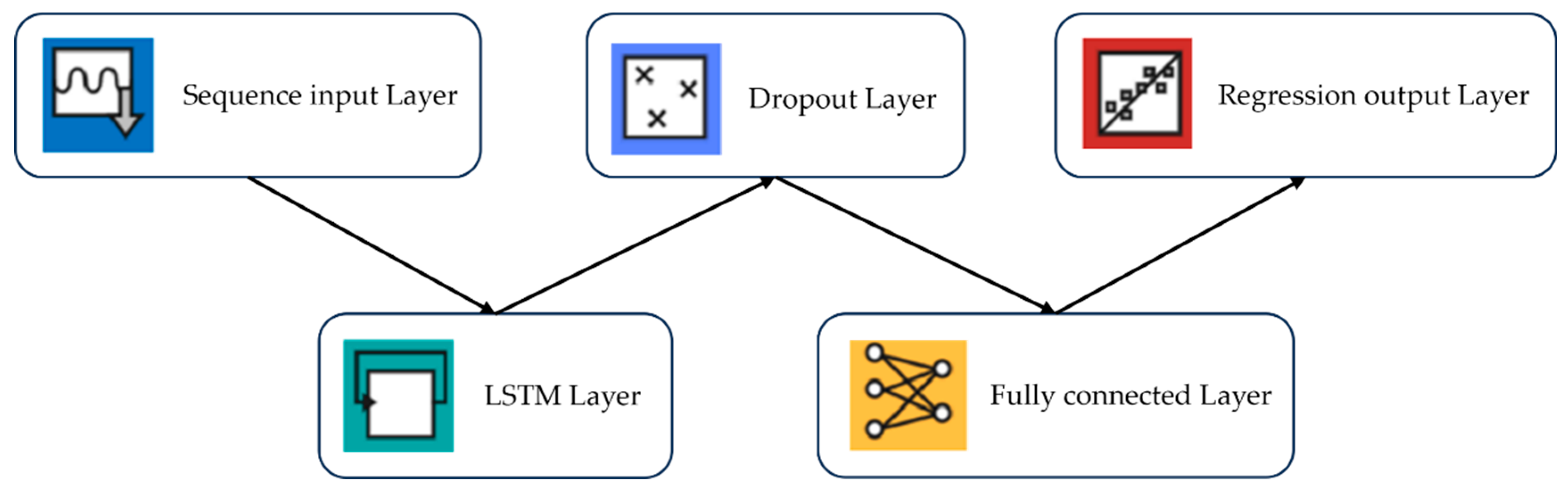
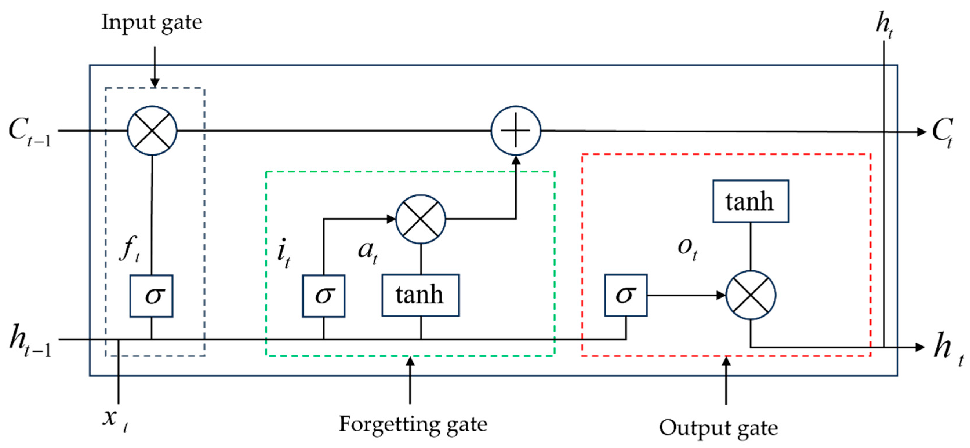
2.3. Long Short-Term Memory (LSTM)

The LSTM network structure is built on the foundation of recurrent neural networks (RNNs) and also includes forget gates, input gates, and output gates, allowing the model to selectively remember relevant information and discard irrelevant information. This structure addresses the issues of gradient explosion and vanishing gradients commonly found in RNNs. The LSTM network model enhances learning of long-term dependencies, enabling it to derive the state at the next time step from the previous state, thus achieving a “memory” function that effectively improves the model’s predictive accuracy.

Figure 3 shows the general single-layer LSTM network’s structure.

For a given sequence, the iterative formulation of the RNN structure is as stated in Equations (7) and (8).

$$h_t=f_a(w_{xh}{x}_t+w_{hh}{h}_{t-1}+b_h)$$

(8)

$$y_t=w_{hy}{h}_t+b_y$$

(9)

where $w$ is the matrix of weight coefficients; $b$ is the bias vector; $f_a$ represents the activation function; and the subscript $t$ denotes the moment.

The basic unit structure of LSTM is shown in Figure 4.

To solve the problem of a vanishing and exploding RNN gradient, the deep neural network, unfolding in time, becomes easy to train by introducing control gates, and its forward computation process is shown in Equations (9)–(13).

$$i_t=\sigma (w_{xi}{x}_t+w_{hi}{h}_{t-1}+w_{ci}{c}_{t-1}+b_i)$$

(10)

$$f_t=\sigma (w_{xf}{x}_t+w_{hf}{h}_{t-1}+w_{cf}{c}_{t-1}+b_f)$$

(11)

$$c_t=f_t{c}_{t-1}+i_t\tanh (w_{xc}{x}_t+w_{hc}{h}_{t-1}+b_c)$$

(12)

$$o_t=\sigma (w_{xo}{x}_t+w_{ho}{h}_{t-1}+w_{co}{c}_t+b_o)$$

(13)

$$h_t=o_t\tanh (c_t)$$

(14)

where $i$ is the input gate; $f$ is the forgetting gate; $c$ represents the cell state; $o$ is the output gate; $w$ stands for the corresponding weight coefficient matrix; $b$ stands for the corresponding bias term; $\sigma$ represents the activation function; and $\tanh$ denotes the hyperbolic tangent activation function.

3. Model Established

3.1. VMD-SSA-LSTM Model Established

Based on the above discussion, this paper constructs a coupled model VMD-SSA-LSTM for use in CMP prediction research. The specific steps of the actual prediction process are as follows.

Step 1: select the first n pieces of information as the model input.

Step 2: use the VMD method to decompose the original sequence to obtain k components.

Step 3: set parameters and finally establish the coupled model SSA-LSTM.

Step 4: input each component into the SSA-LSTM prediction model, respectively, to obtain k prediction models.

Step 5: finally, add up the predicted values of the k prediction models correspondingly to obtain the predicted value of CMP.

3.2. Model Evaluation

How can the quality of a model be assessed? When building and evaluating predictive models, selecting appropriate evaluation metrics is crucial. The accuracy of model predictions and the model’s applicability should be assessed in the context of the data characteristics. In order to test the predictive performance of the LSTM model and the LSTM model optimized by SSA algorithms, this paper uses common metrics such as root-mean-square error [33,34,35] ($RMSE$), mean absolute error [33,35] ($MAE$), and the correlation coefficient [36] ($R^2$) to evaluate the model’s performance. The specific calculation formulas are stated in Equations (15)–(17):

$MAE$ can visualize the degree of average absolute deviation of the predicted value from the true value and is easy to understand.

$$MAE={\displaystyle \frac{1}{n}}{\displaystyle \sum _{i=1}^n\left|\left(y_i-{\widehat{y}}_i\right)\right|}$$

(15)

A smaller $RMSE$ indicates lower prediction errors and higher model accuracy. $RMSE$ quantifies the difference between predicted and true values. It is intuitive and easy to interpret. Furthermore, $RMSE$ is highly sensitive to outliers (i.e., extreme values), making it effective at reflecting the model’s performance in the presence of large errors. This enables $RMSE$ to not only evaluate overall prediction accuracy but also uncover the model’s bias in extreme cases.

$$RMSE=\sqrt{{\displaystyle \frac{1}{n}}{\displaystyle \sum _{i=1}^n{(y_i-{\widehat{y}}_i)}^2}}$$

(16)

It has the following advantages: it is easy to calculate, intuitive to interpret, and unit-independent, and also allows cross-model comparison. $R^2$ is particularly suitable for preliminary evaluation and the selection of regression models, providing a quick performance assessment basis for practical applications. This simple scoring mechanism is intuitive and easy to understand, making it convenient for quickly comparing model performance. The value of $R^2$ ranges from [0, 1], with values closer to 1 indicating better model fit.

$$R^2=1-{\displaystyle \frac{{\displaystyle \sum _{i=1}^n(y_i-{\widehat{y}}_i)}}{{\displaystyle \sum _{i=1}^n(y_i-{\overline{y}}_i)}}}$$

(17)

$$\overline{y}={\displaystyle \frac{1}{n}}{\displaystyle \sum _{i=1}^n{y}_i}$$

(18)

where $y_i$ is the true value, ${\widehat{y}}_i$ is the predicted value, $n$ is the number of test samples, and the formula for $\overline{y}$ is given in Equation (18).

3.3. Parameter Settings

3.3.1. LSTM Initial Hyperparameter Settings

Some model hyperparameter settings are listed in

Table 2. LSTM initial hyperparameter.

Max Epochs	Initial Learn Rate	Learn Rate Drop Period	Learn Rate Drop Factor	L2 Regularization	Hidden-Layer Units
1200	0.005	600	0.2	0.0001	35

.

Adam [37] uses an Initial Learn Rate of 0.005, executes 1200 rounds, uses a first-order moment decay rate of 0.9, a second-order moment decay rate of 0.999, and a decay coefficient 0.2. The author updates the learning rate at 600-round intervals.

The above parameters only reflect the initial values of the model. Continuous testing and modification are needed later to continuously adjust and optimize the parameters to improve the accuracy of the results.

3.3.2. SSA Initial Hyperparameter Settings

In the model, the number of SSA sparrow population is set to 20, and the maximum number of iterations is 20. The producers account for 70%, and the remainder are consumers. The early warning value is 0.8. When the early warning value is less than 0.8, no predator appears; otherwise a predator appears. This is dangerous to the safety of the population, and the population need to go to other places to forage. Scouts constitute 20% of the population. SSA is mainly used in LSTM parameter optimization to find the optimal number of hidden-layer-reaching elements, the maximum training period, and the initial learning rate, where the SSA search ranges are [10, 500], [100, 1200], and [0.001, 0.05], respectively.

3.3.3. VMD Initial Hyperparameter Settings

When the VMD method is used to decompose the original data, the value of modal number K has a great influence on the prediction effect of the model. When the number of modal K decompositions is large, frequency mixing will occur; when the number of decompositions is small, the information of the original signal will be easily lost. The direct observation method can be used to find the best K value by observing the center frequencies corresponding to Intrinsic Mode Function (IMF) plots with different K values and simply distinguishing the dispersion degree of the center frequencies corresponding to different K values. To this end, the IMF plots obtained by VMD with different K values are given in Figure 5.

Direct observation of the optimal K value is challenging due to the complex and often non-obvious relationship between input features and output results. Consequently, determining the best K value through visual inspection or basic analysis is not practical. Instead, the model adopts an iterative approach, comparing predicted outcomes with actual experimental data. By evaluating the prediction accuracy for various K values, the model systematically identifies the outcome that minimizes error and maximizes reliability, thereby ensuring optimal performance for the dataset.

Table 3. Evaluation of model predictions at different values of K.

K	Data	Evaluating Indicator
		RMSE	MAE
7	Train	0.016	0.012
	Test	0.015	0.013
8	Train	0.012	0.009
	Test	0.026	0.022
9	Train	0.018	0.015
	Test	0.025	0.019
10	Train	0.016	0.012
	Test	0.018	0.015

shows the prediction error of the model for different K values of VMD-SSA-LSTM.

As can be seen from the above Table 3, when K = 8, the RMSE and MAE of the model are 0.012 and 0.009 for the training set a, corresponding to the highest model prediction accuracy compared to other K values. In summary, the optimal K value of the VMD-SSA-LSTM model for CMP prediction is 8.

4. Experimental Data Processing and Analysis

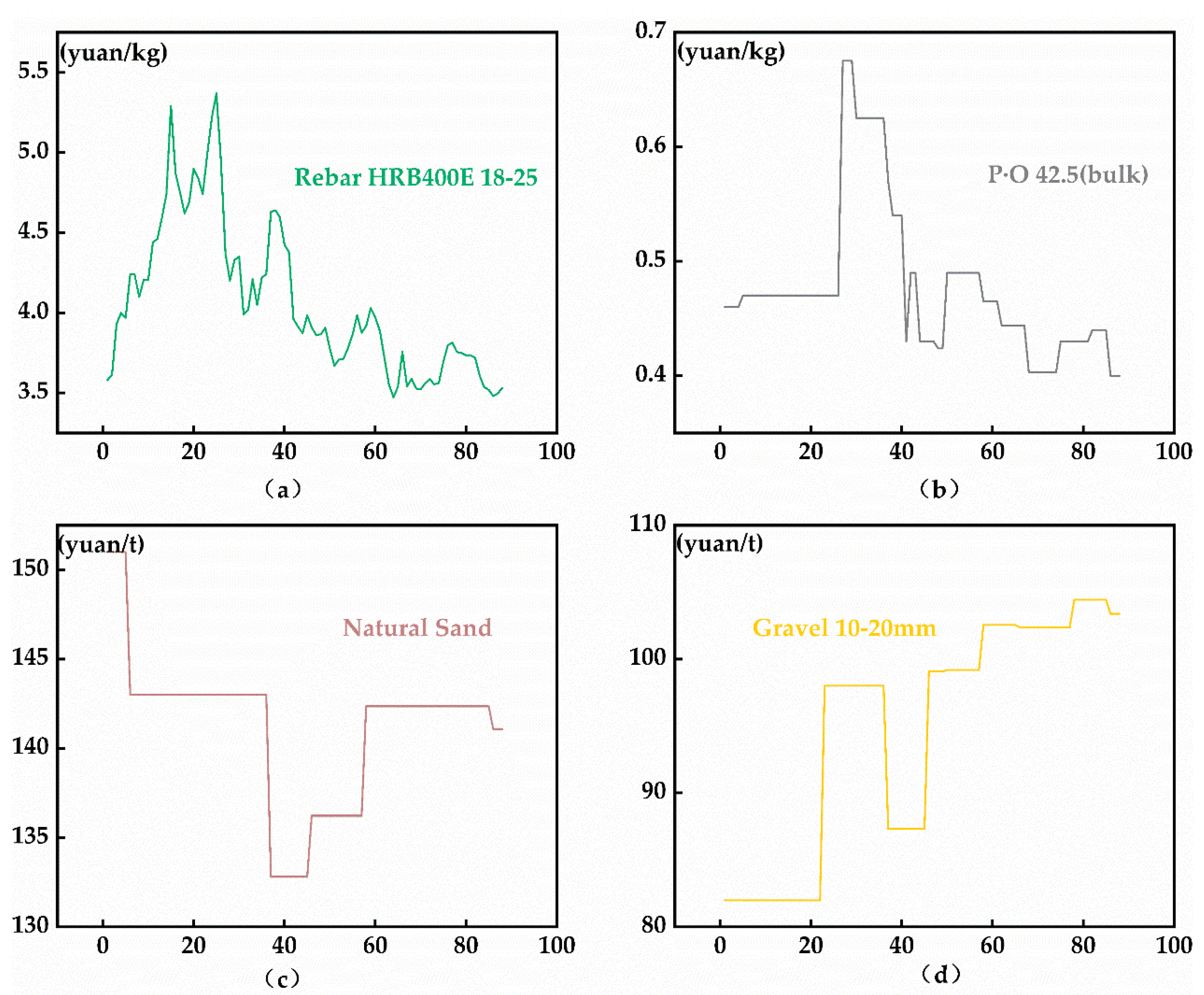
4.1. CMP Analysis

CMP is influenced by various factors, including market demand, supply chain fluctuations, and policy adjustments. The cost of building materials plays a significant role in construction projects, and fluctuations in material prices directly impact project budgets and cost control. Figure 6 shows the price of some construction materials in Hengyang City. The data source is the price information from October 2020 to May 2024 for Hengyang City, as per the General Station of Cost Management of Hunan Department of Housing and Construction. The data are sourced from the Hunan Provincial Construction Engineering Cost Management Station https://zjt.hunan.gov.cn/zjt/hnweb/index.html (accessed on 15 September 2024), which operates under the National Construction Project Cost Data Monitoring Platform. It consists of biweekly data collected and calculated by the cost management departments of various cities and districts in the province, as outlined in the “Biweekly Price Trends for Rebar, Cement, Sand, Gravel, and Concrete Materials”. The prices include the base cost, handling fees, insurance fees, and transportation costs, but exclude VAT. The author compiled and summarized the material price trends specifically for Hengyang City.

This study was approved by the Ethics Committee of the School of Civil Engineering, University of South China. The data were analyzed anonymously and therefore no additional informed consent was required.

From the Figure 6, it can be seen that the CMPs show an irregular and fluctuating phenomenon subject to market constraints. In construction projects, material costs typically account for a large proportion of the project cost. Considering the characteristics of general construction projects, it is evident that construction project investment is substantial and difficult to manage. Many project contractors and builders are prone to fall into a passive state of cost control, resulting in serious cost issues [38]. Since material price fluctuation is one of the most important contributors to deviations from the initial estimated cost in construction projects, the accurate prediction of material costs is essential for the proper management and budgeting of construction projects.

Hence, it is essential to conduct the prediction and analysis of CMP, which is of crucial significance for rationally controlling project costs, ensuring project quality, and guaranteeing project progress.

4.2. Data Pre-Processing

The collected and organized dataset may contain missing values due to human errors or force majeure factors. Additionally, missing data can have a certain impact on the prediction accuracy of the model. Therefore, addressing the missing values in the dataset helps improve data quality, thereby enhancing the model’s predictive accuracy. The specific steps for data preprocessing are as follows.

• Missing data

Missing data can interfere with statistical calculations and model training, increasing errors, and potentially leading to overfitting or underfitting, thereby affecting prediction accuracy. In addition, missing data result in incomplete data, reducing data quality, which in turn affects the accuracy of analysis results and further weakens the model’s performance. To improve data quality and minimize the impact of missing data on the prediction model, the missing data should be filled using the average of the non-missing values from the previous and subsequent periods, based on the characteristics of the experimental data. The calculation formula is as follows Equation (19):

$$\mathrm{D}(x,t)={\displaystyle \frac{D(x-1,t)+D(x+1,t)}{2}}$$

(19)

where $D(x,t)$ represents the filled data value, $x$ is the missing data, $t$ is the corresponding collection point of the missing data, $D(x-1,t)$ are the data at the same time as the previous period of the data point, and $D(x+1,t)$ represent the data at the same time as the next period of the data point.

2.

Normalization data

Normalization, also known as data standardization, is the removal of magnitudes from data. At the same time, normalization helps the data distribution align more closely with the assumptions of the algorithm, speeds up model training, and improves the model’s accuracy and stability. The method used in this paper is Min–Max Scaling. The specific calculation formula is given as Equation (20).

$$x_i={\displaystyle \frac{x-x_{\min }}{x_{\max }-x_{\min }}}$$

(20)

where $x_{\min }$ and $x_{\max }$ are the minimum and maximum values of the dataset, respectively.

5. Model Application and Results Discussion

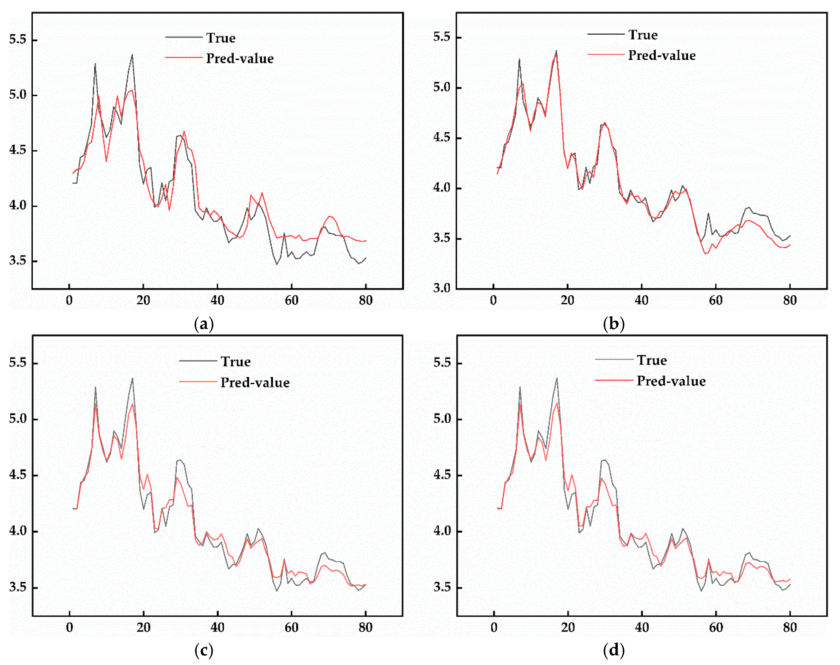
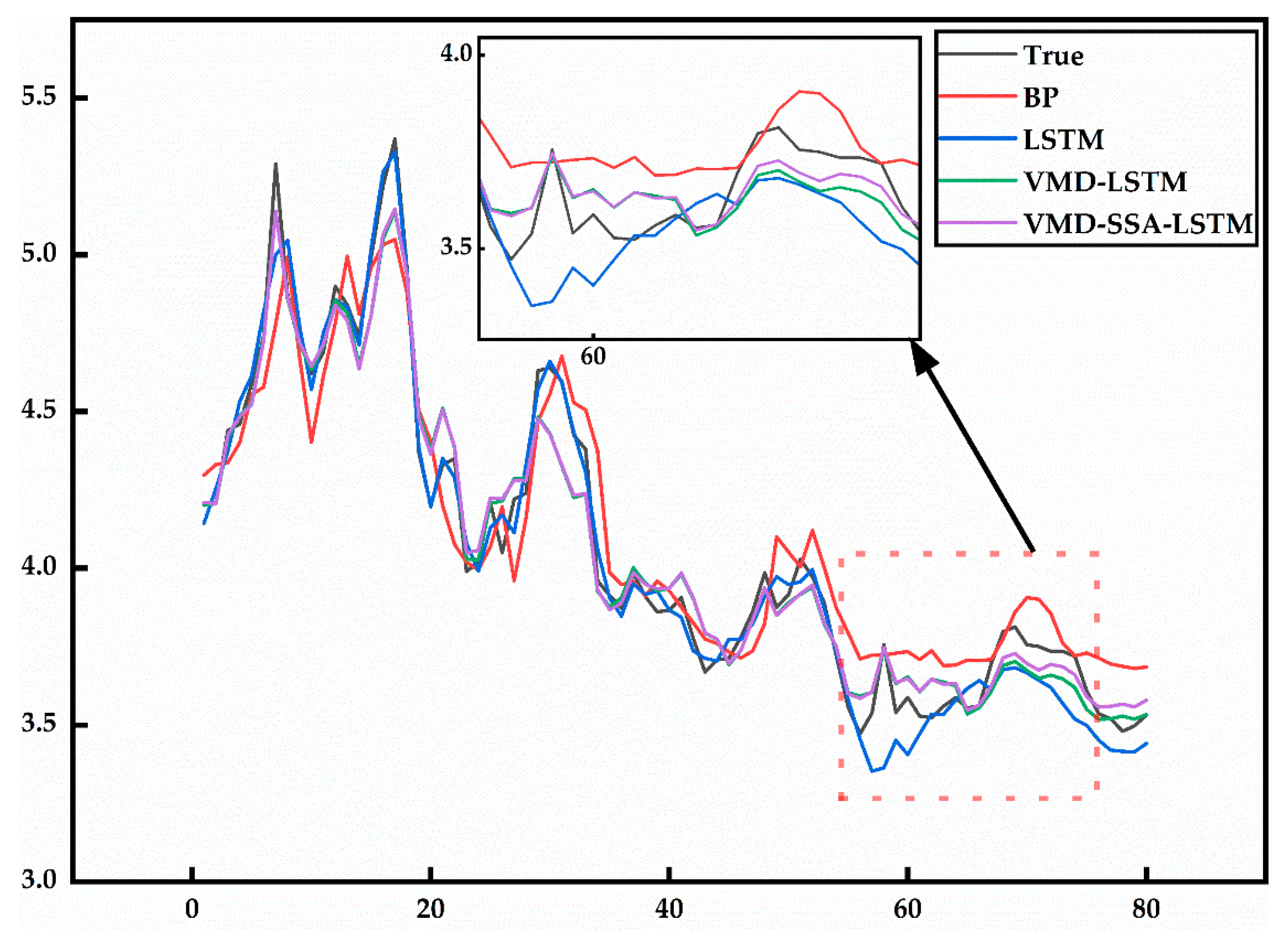
5.1. Model Application Comparison

This paper uses the experimental sample data for the Hunan Housing and Construction Department cost management station, Hengyang City, for 1 October 2020–31 May 2024 based on the re-bar HRB400E 18–25 half-monthly market information price. Using the same experimental data, it is necessary to divide the dataset, with the training set accounting for 70% and the testing set accounting for 30%. Then, the researcher should input the processed experimental data into the established model for prediction to compare and verify the prediction effect and prediction accuracy of the coupled model.

First, a BP neural network prediction model with a topology of 8-5-1 and a single LSTM prediction model are established for prediction. The results and prediction errors of the models are shown in Figure 7 and Figure 8, respectively.

Regarding the prediction results, comparing Figure 7a,b reveals that both the BP model and the LSTM model can approximately predict the change trend of CMP. However, the LSTM model in Figure 7b aligns significantly better with the fluctuation trend of material prices compared to the BP model in Figure 7a. This indicates that the predictive performance of the LSTM model is superior to that of the BP model. In terms of prediction error, the BP model’s error range shown in Figure 8a is [−0.5102, 0.4144], while the LSTM model’s error range in Figure 8b is [−0.3929, 0.1761]. The length of the prediction error interval for the BP model is 0.9246, whereas for the LSTM model it is 0.5690. This means that the prediction error of the LSTM model is reduced by 38.46% compared to the BP model. The variation range of the error interval for the LSTM model is significantly smaller, indicating that the LSTM model has higher prediction accuracy and greater stability in CMP prediction compared to the BP model.

Secondly, the above comparison of single-model predictions shows that while the LSTM model has clear advantages for predicting time series data, its prediction accuracy still does not meet the expected level in the experiment and remains relatively low. To enhance prediction accuracy, VMD is employed to decompose and denoise the original data sequence, thereby improving data quality and achieving better prediction accuracy.

Regarding prediction effect, the VMD-LSTM model in Figure 7c does not show significant improvement compared to the LSTM model in Figure 7b; it may even be considered a case of negative optimization. However, in terms of prediction error, the error range of the LSTM model in Figure 8b is [−0.3929, 0.1761], while the error range of the VMD-LSTM model in Figure 8c is [−0.0716, 0.0327]. The prediction error interval length for the LSTM model is 0.5690, and for the VMD-LSTM model it is 0.1043. The prediction error of the VMD-LSTM model is thus reduced by 81.66% compared to the LSTM model. The variation range of the error interval for the VMD-LSTM model is significantly smaller, indicating that the model is more stable.

Simultaneously, to avoid the negative impact of the observed negative optimization while improving prediction accuracy, SSA is used to optimize the hyperparameters of the LSTM model. The experimental results for the VMD-SSA-LSTM model are shown in Figure 7d and Figure 8d. In terms of prediction error, the error range of the VMD-LSTM model in Figure 8a is [−0.0716, 0.0327], while the error range of the VMD-SSA-LSTM model in Figure 8b is [−0.0444, 0.0228]. The prediction error interval length for the VMD-LSTM model is 0.1043, and it is 0.0672 for the VMD-SSA-LSTM model. The prediction error of the VMD-SSA-LSTM model is reduced by 35.57% compared to the LSTM model. Additionally, the VMD-SSA-LSTM model in Figure 7d does not exhibit negative optimization compared to the VMD-LSTM model in Figure 7c.

5.2. Results Discussion

To verify the superiority of the VMD-SSA-LSTM material price prediction model proposed in this paper, as well as the necessity of VMD decomposition and the effectiveness of SSA in optimizing parameters, and to further clarify that the proposed method has significant improvement and enhancement in predicting CMP it is necessary to select the historical price information data of threaded steel bars in CMP as the experimental sample, and use the BP, LSTM, VMD-LSTM, and VMD-SSA-LSTM models for prediction. Then, the researcher should compare the four prediction models. Figure 9 shows the comparison of the prediction effects of the four models. Figure 10a is an error curve graph of the prediction results of the four models, and Figure 10b is the error box plot of the prediction results of the four models.

Table 4. Prediction effects of various models.

Model	$\mathit{R}\mathit{M}\mathit{S}\mathit{E}$	$\mathit{M}\mathit{A}\mathit{E}$	${\mathit{R}}^2$/%
BP	0.1543	0.1271	89.966
LSTM	0.0935	0.0681	96.315
VMD-LSTM	0.0932	0.0712	96.336
VMD-SSA-LSTM	0.0907	0.0699	96.532

shows the comparison of the evaluation index results of all models in the performance of the same experimental sample.

From the analysis of the chart and table above, the locally enlarged view indicated by the arrow in Figure 9 shows that all four models exhibit relatively good fitting effects, with the VMD-SSA-LSTM model performing the best. The error curve in Figure 10a indicates that the prediction error range for those models is within [−0.6, 0.4]. Additionally, the error box plot in Figure 10b reveals that the BP model has the largest error and fluctuates significantly, while the prediction error of the VMD-SSA-LSTM model is the smallest, demonstrating a stable curve trend that indicates high stability. For the LSTM model (i.e., VMD-SSA-LSTM) optimized by VMD decomposition and SSA parameters, the $RMSE$ and $MAE$ are reduced by 2.68% and 1.82%, respectively, compared to the VMD-LSTM model; by 2.99% and −2.57%, respectively, compared to the single LSTM model; and by 41.22% and 45%, respectively, compared to the BP model. Furthermore, the $R^2$ values increase by 0.196%, 0.217%, and 6.566%, respectively. This demonstrates that the VMD-SSA-LSTM model effectively improves prediction accuracy by enhancing data quality through VMD and optimizing LSTM parameters using SSA.

The empirical results demonstrate that the VMD-SSA-LSTM model achieves significant improvements in prediction accuracy over traditional models. Key findings include the following:

• The model’s RMSE is reduced by 41.22% compared to the BP model and by 2.99% compared to the standalone LSTM model, indicating superior performance in capturing complex price patterns.
• The R² value for the VMD-SSA-LSTM model is 96.532%, showcasing its robustness in fitting observed data.

From a practical perspective, these results highlight the model’s utility in real-world scenarios. For instance, construction managers can leverage the improved predictive accuracy to prepare more precise budgets and mitigate financial risks associated with material price volatility. Moreover, the model’s ability to process noisy data ensures reliability across diverse market conditions, making it a valuable tool for strategic planning. Unlike conventional models, which often struggle with noisy and nonlinear data, the VMD-SSA-LSTM framework effectively addresses these challenges. The integration of VMD enhances data quality by isolating noise, while SSA optimizes LSTM’s learning process, leading to more accurate and stable predictions. These improvements align with previous findings on the benefits of hybrid models but extend their application to the underexplored domain of CMP forecasting.

6. Conclusions

Material price prediction is crucial for managing cost risks in engineering projects. It aids in accurately preparing budgets and formulating strategies to optimize the cost structure, ensuring that project budgets remain controllable. By optimizing the supply chain, identifying price risks, and formulating corresponding countermeasures, it effectively reduces the risks of cost fluctuations and ensures project progress. Additionally, it provides a foundation for investment decisions, enabling enterprises to enhance their competitiveness through optimized quotations and improved reputations. Furthermore, it encourages innovation to reduce costs, thereby strengthening enterprises’ ability to manage cost risks [3,7,9,10,11] and facilitating the smooth progression of engineering projects.

This paper introduces a novel hybrid prediction model, VMD-SSA-LSTM, for CMP forecasting. Empirical validation and model comparisons show that the proposed model significantly enhances both prediction accuracy and goodness of fit. The findings are highly relevant for stakeholders in the construction industry, particularly in terms of cost risk management, budget planning, and decision-making. The key conclusions are as follows:

• A novel framework is developed for CMP forecasting that surpasses traditional methods in both accuracy and stability. By employing VMD to decompose and denoise the data, critical features are extracted, enhancing data quality and mitigating the limitations of single-model approaches that often result from insufficient data learning. Furthermore, SSA addresses issues like rapid convergence and local optima, complementing the LSTM model and significantly improving its predictive performance and robustness.
• The constructed VMD-SSA-LSTM prediction model shows a reduction in RMSE of 2.68% compared to the VMD-LSTM model, 2.99% compared to the single LSTM model, and 41.22% compared to the BP model. Additionally, the R² values increase by 0.196%, 0.217%, and 6.566%, respectively. The model enhances budget accuracy by reducing material price prediction errors by over 40% compared to traditional methods, leading to better financial planning and fewer cost overruns.
• Risk mitigation and strategic planning: accurate forecasts allow companies to proactively manage risks by locking in prices or adjusting project schedules, minimizing financial uncertainties and delays.
• Optimized resource allocation and bidding: the model’s improved predictive accuracy supports efficient resource allocation, competitive bidding, and strategic procurement, helping firms stay within budget and maintain profitability.

This study confirms the practicality of the VMD-SSA-LSTM model in CMP prediction, broadening the application scope of deep learning technologies in this domain. Future research could explore the extension of this approach to other industries or the integration of additional optimization techniques to enhance predictive accuracy further. The proposed hybrid prediction method holds significant reference value for advanced studies in project cost risk management, showcasing strong potential for practical implementation and substantial engineering value.

References

1. Barg, S.; Flager, F.; Fischer, M. An analytical method to estimate the total installed cost of structural steel building frames during early design. J. Build. Eng. 2018, 15, 41–50. [Google Scholar] [CrossRef]
2. Tao, X.; Li, Y. Research on risk management of material price in engineering cost control. Constr. Econ. 2006, 7, 73–75. [Google Scholar]
3. Bayram, S.; Al-Jibouri, S. Efficacy of estimation methods in forecasting building projects’ costs. J. Constr. Eng. Manag. 2016, 142, 05016012. [Google Scholar] [CrossRef]
4. Wang, X.; Xing, L. Significant project cost estimation method based on BP neural network. People’s Yellow River 2011, 33, 115–116+119. [Google Scholar]
5. Weidman, J.E.; Miller, K.R.; Christofferson, J.P.; Newitt, J. Best practices for dealing with price volatility in commercial construction. Int. J. Constr. Educ. Res. 2011, 7, 276–293. [Google Scholar] [CrossRef]
6. Hwang, S.; Park, M.; Lee, H.S.; Kim, H. Automated time-series cost forecasting system for construction materials. J. Constr. Eng. Manag. 2012, 138, 1259–1269. [Google Scholar] [CrossRef]
7. Shahandashti, S.M.; Ashuri, B. Forecasting engineering news-record construction cost index using multivariate time series models. J. Constr. Eng. Manag. 2013, 139, 1237–1243. [Google Scholar] [CrossRef]
8. Lu, Y.; Nie, C.; Zhou, D.; Shi, L. Research on programmatic multi-attribute decision-making problem: An example of bridge pile foundation project in karst area. PLoS ONE 2023, 18, e0295296. [Google Scholar] [CrossRef]
9. Joukar, A.; Nahmens, I. Volatility forecast of construction cost index using general autoregressive conditional heteroskedastic method. J. Constr. Eng. Manag. 2016, 142, 04015051. [Google Scholar] [CrossRef]
10. Cao, M.T.; Cheng, M.Y.; Wu, Y.W. Hybrid computational model for forecasting Taiwan construction cost index. J. Constr. Eng. Manag. 2015, 141, 04014089. [Google Scholar] [CrossRef]
11. Elfahham, Y. Estimation and prediction of construction cost index using neural networks, time series, and regression. Alex. Eng. J. 2019, 58, 499–506. [Google Scholar] [CrossRef]
12. Mir, M.; Kabir, H.M.D.; Nasirzadeh, F.; Khosravi, A. Neural network-based interval forecasting of construction material prices. J. Build. Eng. 2021, 39, 102288. [Google Scholar] [CrossRef]
13. Yip, H.; Fan, H.; Chiang, Y. Predicting the maintenance cost of construction equipment: Comparison between general regression neural network and Box–Jenkins time series models. Autom. Constr. 2014, 38, 30–38. [Google Scholar] [CrossRef]
14. Graves, A. Long short-term memory. In Supervised Sequence Labelling with Recurrent Neural Networks; Springer: Berlin/Heidelberg, Germany, 2012; pp. 37–45. [Google Scholar]
15. Jiang, J.; Qi, C.; Bo, B.; Li, P. Research on Prediction of Construction Material Prices Based on BP Neural Network. Proj. Manag. Technol. 2022, 20, 24–27. [Google Scholar]
16. Ouyang, H.; Li, X.; Zhang, X. Application of Artificial Neural Network in the Prediction of Building Material Prices. J. Wuhan Univ. Technol. (Inf. Manag. Eng.) 2013, 35, 115–118. [Google Scholar]
17. Wang, Y. Major Material Price Forecast based on GM (1,1) Grey Dynamic Model in Tender Offer. Railw. Eng. Technol. Econ. 2013, 28, 39–43. [Google Scholar]
18. Suad, H.; Elshaimaa, E.; Hossam, H. Prediction of construction material prices using ARIMA and multiple regression models. Asian J. Civ. Eng. 2023, 24, 1697–1710. [Google Scholar]
19. Wang, J.; Fang, X. Price prediction of mass engineering materials based on ARIMA construction research. Eng. Cost Manag. 2020, 65–75. [Google Scholar] [CrossRef]
20. Wang, J.; Wang, C. Analysis and Prediction of Building Material Prices. Energy Conserv. 2015, 34, 7–10. [Google Scholar]
21. Nguyen, V.H.; Naeem, A.M.; Wichitaksorn, N.; Pears, R. A smart system for short-term price prediction using time series models. Comput. Electr. Eng. 2019, 76, 339–352. [Google Scholar] [CrossRef]
22. Peng, Y.; Liu, Y.; Zhang, R. Modeling and analysis of stock price forecast based on LSTM. Comput. Eng. Appl. 2019, 55, 209–212. [Google Scholar]
23. Huang, C.; Cheng, X. Research on Stock Price Prediction Based on LSTM Neural Network. J. Beijing Inf. Sci. Technol. Univ. (Sci. Technol. Ed.) 2021, 36, 79–83. [Google Scholar] [CrossRef]
24. Fang, J.; Liu, H.; Hu, Y. Soybean Futures Price Prediction Based on LSTM Deep Learning. Prices Mon. 2021, 7–15. [Google Scholar] [CrossRef]
25. Tu, J.; Liu, Y.; Zhou, M.; Li, R. Prediction and analysis of compressive strength of recycled aggregate thermal insulation concrete based on GA-BP optimization network. J. Eng. Des. Technol. 2021, 19, 412–422. [Google Scholar] [CrossRef]
26. Luo, Z.; Bu, Y. Research on Price Forecast Method of Building Materials Based on Grey Neural Network PGNN Model. Constr. Econ. 2020, 41, 115–120. [Google Scholar] [CrossRef]
27. Shiha, A.; Dorra, M.E.; Nassar, K. Neural Networks Model for Prediction of Construction Material Prices in Egypt Using Macroeconomic Indicators. J. Constr. Eng. Manag. 2020, 146, 04020010. [Google Scholar] [CrossRef]
28. Tang, B.; Han, J.; Guo, G.; Yi, C.; Sai, Z. Building material prices forecasting based on least square support vector machine and improved particle swarm optimization. Archit. Eng. Des. Manag. 2019, 15, 196–212. [Google Scholar] [CrossRef]
29. Dragomiretskiy, K.; Zosso, D. Variational mode decomposition. IEEE Trans. Signal Process. 2013, 62, 531–544. [Google Scholar] [CrossRef]
30. Xue, J.; Shen, B. A novel swarm intelligence optimization approach: Sparrow search algorithm. Syst. Sci. Control. Eng. 2020, 8, 22–34. [Google Scholar] [CrossRef]
31. Wang, J.; Li, X.; Zhou, X.; Zhang, K. Ultra-short-term wind speed prediction based on VMD-LSTM. Power Syst. Prot. Control 2020, 48, 45–52. [Google Scholar] [CrossRef]
32. Zhao, J.; Chi, Y.; Zhou, Y. Short-term power load forecasting based on SSA-LSTM model. Adv. Technol. Electr. Eng. Energy 2022, 41, 71–79. [Google Scholar]
33. Willmott, C.J.; Matsuura, K. Advantages of the mean absolute error (MAE) over the root mean square error (RMSE) in assessing average model performance. Clim. Res. 2005, 30, 79–82. [Google Scholar] [CrossRef]
34. Wang, Z.; Bovik, C.A. Mean squared error: Lot it or leave it? A new look at Signal Fidelity Measures. IEEE Signal Process. Mag. 2009, 26, 98–117. [Google Scholar] [CrossRef]
35. Chai, T.; Draxler, R. Root mean square error (RMSE) or mean absolute error (MAE)?—Arguments against avoiding RMSE in the literature. Geosci. Model Dev. 2014, 7, 1247–1250. [Google Scholar] [CrossRef]
36. Cameron, A.C.; Windmeijer, F.A.G. An R-squared measure of goodness of fit for some common nonlinear regression models. J. Econom. 1997, 77, 329–342. [Google Scholar] [CrossRef]
37. Kingma, D.; Ba, J. Adam: A Method for Stochastic Optimization. arXiv 2014, arXiv:1412.6980. [Google Scholar] [CrossRef]
38. Chen, T.; Wang, Y. Analysis of Budget and Control of New Green Buildings’ Project Cost. Eng. Econ. 2015, 31–36. [Google Scholar] [CrossRef]
Figure 1. The flow chart of VMD.
Applsci 15 02005 g001
Figure 2. The flow chart of SSA.
Applsci 15 02005 g002
Figure 3. LSTM network structure.
Applsci 15 02005 g003
Figure 4. LSTM basic unit structure.
Applsci 15 02005 g004
Figure 5. Intrinsic Mode Function. (a) The value of the modal function K is 7. (b) The value of the modal function K is 8. (c) The value of the modal function K is 9. (d) The value of the modal function K is 10.
Applsci 15 02005 g005
Figure 6. The prices of some construction materials in Hengyang. (a) The graph shows historical information price data for Rebar HRB400E 18–25. (b) The graph shows historical information price data for Ordinary Silicate Cement (P-O) 42.5 (bulk). (c) The graph shows historical information price data for Natural Sand. (d) The graph shows historical information price data for Gravel 10–20 mm.
Applsci 15 02005 g006
Figure 7. Prediction results of four models. (a) The graph represents the trend of change between the predicted and true values of the BP model, i.e., the BP model fit. (b) The graph represents the trend of change between the predicted and true values of the LSTM model, i.e., the LSTM model fit. (c) The graph represents the trend of change between the predicted and true values of the VMD-LSTM model, i.e., the VMD-LSTM model fit. (d) The graph represents the trend of change between the predicted and true values of the VMD-SSA-LSTM model, i.e., the VMD-SSA-LSTM model fit.
Applsci 15 02005 g007
Figure 8. The model’s prediction error. (a) The graph represents the error range and error fluctuations between the BP model’s prediction error and the true value. (b) The graph represents the error range and error fluctuations between the LSTM model’s prediction error and the true value. (c) The graph represents the error range and error fluctuations between the VMD-LSTM model’s prediction error and the true value. (d) The graph represents the error range and error fluctuations between the VMD-SSA-LSTM model’s prediction error and the true value.
Applsci 15 02005 g008
Figure 9. Comparison of prediction results of four models.
Applsci 15 02005 g009
Figure 10. The comparison of prediction results errors of four models. (a) The comparison of standard errors of the 4 prediction models’ curve plot. (b) Box line plots of standard error comparisons for each prediction model, representing the distribution of model prediction data.
Applsci 15 02005 g010