Research on the Time Series Prediction of Acoustic Emission Parameters Based on the Factor Analysis–Particle Swarm Optimization Back Propagation Model

Abstract

Early warning for rock blasting is crucial for ensuring the safety of deep underground engineering. Existing methods primarily focus on classifying rock blasting levels, which makes it difficult to provide timely warnings. This paper proposes a novel early warning framework for rock blasting based on time series prediction of acoustic emission (AE) parameters. Based on uniaxial rock tests, ten AE parameters (rise time, ring count, energy, duration, amplitude, average frequency, RMS voltage, average signal level, peak frequency, and initial frequency) are identified as potential indicators for rock blasting early warning. These ten parameters collectively affect the accuracy of AE monitoring. Factor analysis is employed to process the normalized AE data, simplifying the data structure and identifying common variables. Additionally, it is found that the BP neural network optimized by Particle Swarm Optimization (PSO) is more suitable for predicting the future evolution of these AE parameters. This makes it possible to establish a comprehensive multi-indicator early warning system. The proposed framework provides a new perspective for rock blasting early warning systems.

1. Introduction

Rockburst, a geological hazard phenomenon that is a key concern in the fields of underground engineering and rock mechanics, refers to the brittle fracture and failure that occurs suddenly in the exposed rock mass in deep underground mining areas or regions with high tectonic stress. The underlying cause is the instantaneous, violent, and unreserved release of the strain energy accumulated within the exposed rock mass, which leads to a brittle fragmentation state of the rock mass similar to that caused by an explosive impact. The accompanying phenomenon of rockburst-induced pressure not only causes a large amount of rock to collapse and peel off, generating intense acoustic effects and impactful air waves that can damage the internal facilities of the mine, but the seismic waves generated can also propagate outward and pose a threat to the stability of surface buildings [1,2]. In view of this, how to effectively control rockburst has become a core problem in the fields of underground engineering and rock mechanics.

At present, numerous scientific research efforts focus on uncovering the underlying physical mechanisms behind rockburst phenomena and, at the same time, strive to formulate forward-looking prediction strategies and practical prevention measures, aiming to anticipate the probability of rockburst occurrence in advance and minimize its negative impacts. At this stage, by leveraging advanced deep learning frameworks to construct a quantitative risk assessment model for rockburst, it provides technical support for accurately measuring the probability of such events [3].

In terms of rock mass monitoring techniques, acoustic emission monitoring and microseismic monitoring are two commonly used conventional methods in the industry [4]. The high–frequency part of the signal spectrum captured by AE monitoring is distributed in the range of 10⁴ to 10⁷ Hz [5]. With this characteristic, this technique has unique advantages in the study of the fracture process of rocks on a micro-scale [6] and has become a commonly used monitoring method in laboratory rockburst simulation tests. In contrast, the operating frequency range of MS monitoring is between 10⁻¹ and 10⁻³ Hz [7]. Based on its high-sensitivity ability to capture the dynamic responses of large-scale rock masses, this technique is more often applied to the monitoring of rock mass stability at actual engineering sites. It is worth noting that, during the laboratory rockburst simulation tests relying on AE monitoring, researchers have found that high-amplitude AE signals are often difficult to detect on the eve of a rockburst [8]. At the same time, the fractal dimension index of AE signals shows a dynamic change characteristic of first rising steadily and then dropping sharply over time [9].

An in-depth analysis of AE spectrum evolution is crucial for evaluating and predicting rockburst risk. When it shows a low amplitude, wide band, and multi-peaks, the dominant frequency decreases [9] and the band shifts from a low to high frequency [10]. He et al.’s team [11] found via studies that, when AE energy deviation rises and the daily high-energy sum peaks, rockburst is imminent. Also, sandstone AE location-monitoring shows increased high-energy AE events and inflection points in variance curves of AE rise time/amplitude and AF, and rise time and duration curves can serve as key precursors [12]. The AE signals in the rockburst process possess distinct TS characs. Currently, the industry usually uses advanced algorithm tools like GRNN [13], SVM [14], LW C4.5 Alg [15], RF, AdaBoost, GBDT, XGBoost, and LGBM [16] for the processing and analysis of such signals. Although these methods previously showed good predictive accuracy, they have inherent flaws that are hard to overcome by conventional options, e.g., a grey predictive model requires stable data, so its effect drops for volatile data; SVM has difficulty in operating key parameters during modeling; conventional neural nets converge slowly and tend to become stuck in local optima due to gradual descent limits; wavelet analysis has a complex calculation process. How to select a prediction method suitable for the time series characteristics of AE is also one of the key issues that requires solving in the current rockburst research field. In order to effectively improve the actual performance of the above-mentioned various prediction models, researchers have innovatively introduced a target weighting strategy and combined it with the Particle Swarm Optimization algorithm [17,18,19].

After discretizing the original rockburst monitoring data, fine-grained dynamic adjustments are made to the weights of the various parameters input into the model. Facing dataset imbalance due to sample size differences in rockburst cases, researchers adopted advanced data-augmentation techniques like random oversampling [20] and SMOTE to optimize the original dataset, enhancing the model’s generalization in complex conditions [21,22]. Researchers used the Random Gradient Boosting model to classify rockburst damage in a 254-event database and received five predictive indicators [23,24]. Ma [25] proved that, after dataset optimization, the model based on Borderline-SMOTE1 and Adaboost had significantly better prediction accuracy. Although deep learning for rockburst intensity prediction is quite advanced, research on predicting future trends of rockburst-related parameters based on monitoring data time series changes is still in its infancy. By combining enhanced CNN with dynamic sliding window technology, a model to capture rockburst evolution trends and predict microseismic parameters or combinations is expected [26]. The BiLSTM, with its unique mechanisms, can identify and classify microseismic, AE, and EMR signals related to rockburst [27,28,29].

Addressing the aforementioned issues, the author proposes a fundamental approach to predicting rockbursts using AE time series. Firstly, factor analysis is utilized to reduce the dimensionality of AE characteristic parameters, eliminating redundant information, and the reorganized parameters are used as observation indicators for the AE time series prediction model. Subsequently, a Back Propagation (BP) neural network is employed to establish an AE data prediction model. To mitigate the poor prediction performance caused by initial weights and thresholds when BP networks process large-scale time series, a related fitness function can be established, and the Particle Swarm Optimization (PSO) algorithm is used to optimize the weights and thresholds of the BP neural network, ultimately achieving better prediction results. Finally, a performance analysis of the FA-PSOBP AE time series model is conducted.

2. Materials and Methods

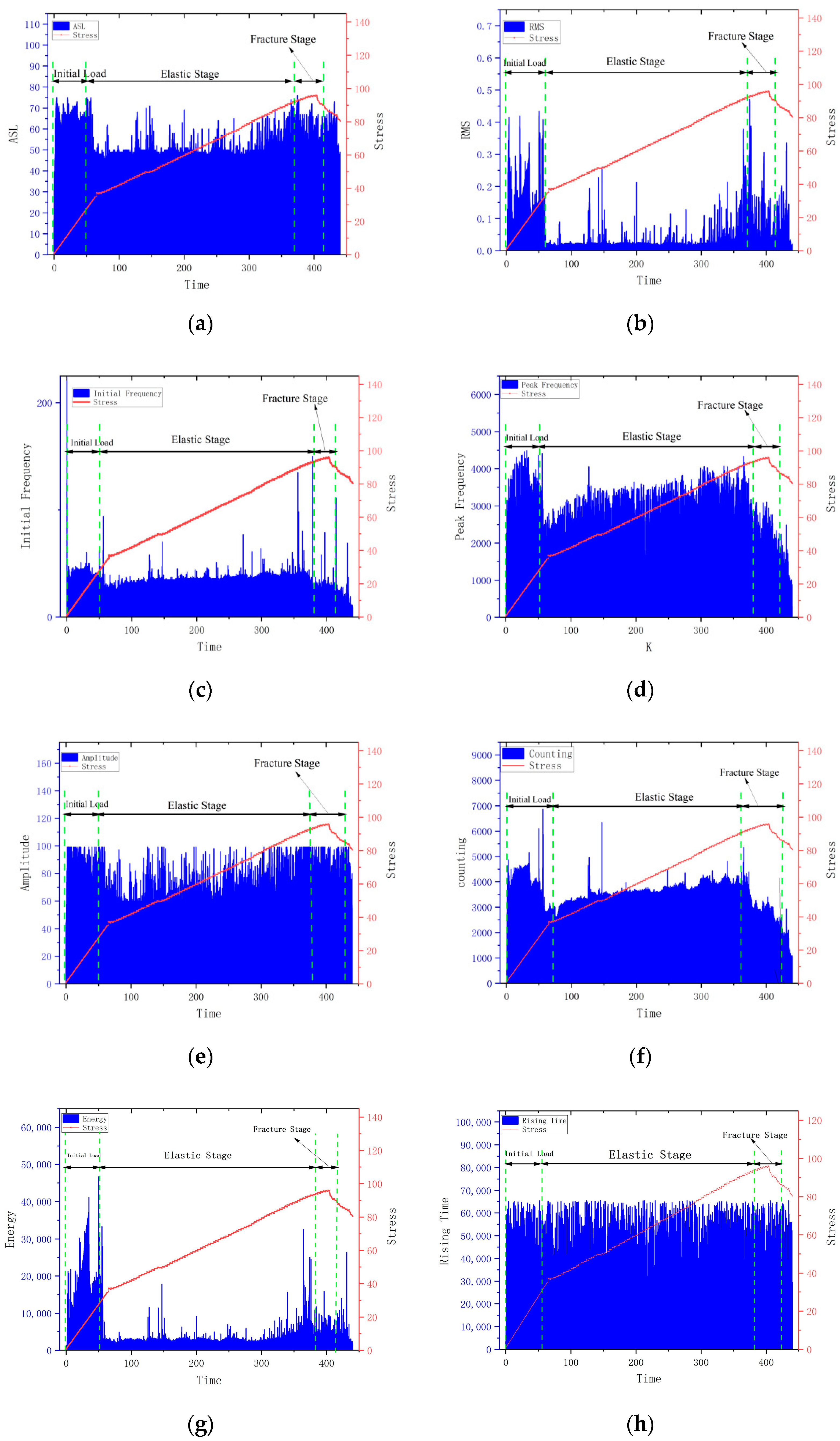
2.1. Determination of Acoustic Emission Parameters

The pressure machines used for the acoustic emission (AE) tests on rocks under uniaxial compression are INSTRON 1346 electro-hydraulic servo-controlled rigid material testing machines, while those for AE tests on rocks under indirect tensile stress are INSTRON 1342 electro-hydraulic servo-controlled rigid material testing machines. The AE instrument used to measure AE parameters during rock loading is the PCI-2 multi-channel AE testing system produced by the Physical Acoustics Corporation (PAC) in the United States. The AE sensors are R6α resonant high-sensitivity sensors. The AE instrument and sensors are shown in Figure 1. The rock samples used in this study were collected from the vicinity of the 307 stope at the −70 m level with the sample F1-1. The samples are cuboid in shape, with dimensions of 53.65 mm × 52.30 mm × 99.50 mm, a weight of 849 g, and a density of 3.04 g/cm³. The samples exhibit good integrity and show slight weathering on the surface, indicating that their physical properties have not been significantly affected by environmental factors. The samples were stored at the stope for approximately 1–2 years prior to testing, during which they were not subjected to significant mechanical damage or chemical erosion. The number of samples collected meets the requirements for specimen processing, ensuring the reliability and representativeness of the experimental data. As shown in Figure 2, Vaseline was used for coupling between the samples and the AE sensors, and electrical tape was used for fixation. The samples were continuously loaded under uniaxial compression until complete failure, with displacement control and a loading rate of 0.005 mm/s. The AE monitoring instrument had a sampling frequency of 1 MHz and a threshold value of 40 dB, and the AE sensors had a resonant frequency of 150 kHz. The changes in AE events, energy, load, duration, and other parameters during the failure process of the samples were recorded.

As shown in Figure 3, the curve illustrates that the intensity of acoustic emission (AE) activity has good consistency with the trend of load variation.

In acoustic emission (AE) research, it is common to randomly select variables for analysis without exploring the correlation between each variable. Factor analysis is a multivariate statistical method that starts with studying the internal correlation and dependence among variables, and it reduces a number of complexly related variables into a few comprehensive factors. The basic idea of factor analysis is to classify observed variables by grouping those with high correlation, i.e., closely related variables, into the same category, while variables in different categories have low correlation. Each category of variables thus represents a basic structure, known as a common factor. The goal of factor analysis in the context of the studied problem is to describe each original observed variable as a linear function of the smallest possible number of unobservable common factors plus a unique factor.

2.2. Data Preprocessing

Due to the different dimensions of various indicators, which make them incomparable, it is necessary to standardize the original data to eliminate the influence of these dimensions. The standardization formula is as follows:

$$x_{st}={\displaystyle \frac{x-x_{\min }}{x_{\max }-x_{\min }}}$$

(1)

In the formula, $x$ represents the original data and $x_{st}$ represents the standardized data.

2.2.1. Adaptability Analysis

We selected 200 acoustic emission signals as sample data and set the characteristic parameters as rise time d1, ring count d2, energy d3, duration d4, amplitude d5, average frequency d6, RMS voltage d7, average signal level d8, peak frequency d9, and initial frequency d10, denoted as D = (d1, d2, d3, d4, d5, d6, d7, d8, d9, d10). To verify whether these data are suitable for factor analysis, we conducted a Kaiser–Meyer–Olkin (KMO) test and Bartlett’s test of sphericity and assessed the Sig value and KMO value. The results are shown in

Table 1. Results of KMO and Bartlett’s Test of Sphericity.

KMO and Bartlett’s Test
Kaiser–Meyer–Olkin Measure of Sampling Adequacy		0.842
Bartlett’s test of sphericity	Approximate Chi-Square	151,302.068
	Degree of freedom	45
	Significance	0.000

.

In Table 1, the KMO value is 0.842, which is greater than the critical value of 0.6, indicating that the data are suitable for factor analysis. Additionally, the results of Bartlett’s test of sphericity show a significance level of 0.000, which is less than the standard of 0.05. Therefore, the data are appropriate for factor analysis.

The following is a description of the scree plot, as shown in Figure 4:

The scree plot displays the components (variables) on the horizontal axis and the corresponding eigenvalues of the indicator variables on the vertical axis. The eigenvalues are arranged in descending order. As shown in the plot, there is a steep slope from the first to the second indicator, with a noticeable inflection point at the third factor. The subsequent indicator variables gradually form a relatively flat curve. This suggests that selecting three factors is appropriate.

2.2.2. Extraction of Common Factors

Using SPSS (version 27), we obtained the characteristic values and variance contribution rates for each factor (see table below).

In

Table 2. Total variance explained.

Ingredients	Initial Eigenvalues			Extract the Sum of Squares of the Loadings			Sum of the Rotating Load Squares
	Total	Percentage Variance	Accumulate %	Total	Percentage Variance	Accumulate %	Total
1	5.696	56.955	56.955	5.696	56.955	56.955	4.104
2	1.476	14.756	71.711	1.476	14.756	71.711	2.509
3	1.019	10.186	81.898	1.019	10.186	81.898	1.577
4	0.462	4.625	86.523
5	0.443	4.427	90.950
6	0.343	3.433	94.383
7	0.298	2.981	97.364
8	0.132	1.317	98.681
9	0.094	0.937	99.618
10	0.038	0.382	100.000

, we can see that the first three factors explain 81.898% of the total variance. This means that the three extracted common factors can represent 81.898% of the original 10 indicators that measure the characteristics of acoustic emission energy. This indicates that there is relatively little loss of data information and that the initial data can be well explained. Therefore, we extract three common factors as Y1, Y2, and Y3. By performing weighted calculations on these factors, we can obtain a comprehensive scoring model Y.

The three common factors (Y1, Y2, Y3) extracted through factor analysis correspond to composite indicators for the dimensions of energy, time, and frequency, respectively:

Y1 (Energy Factor): Composed of energy, amplitude, and average signal intensity, it reflects the trend of energy accumulation during rock mass failure.

Y2 (Time Factor): Consisting of duration, rise time, and ring-down count, it characterizes the temporal evolution pattern of failure events.

Y3 (Frequency Factor): Made up of peak frequency and initial frequency, it indicates the dynamic changes in failure frequency.

Collectively, these three factors explain 81.9% of the total variance, effectively encapsulating the physical meanings of the original 10 parameters.

As shown in

Table 3. Factor Loadings and interpretation of acoustic emission parameters.

Parameter	Y1 (Energy-Related)	Y2 (Time-Related)	Y3 (Frequency-Related)
Energy (d3)	0.92	0.15	0.08
Amplitude (d5)	0.88	0.21	0.12
Average Signal Strength (d8)	0.85	0.18	0.09
Duration (d4)	0.13	0.91	0.07
Rise Time (d1)	0.11	0.89	0.05
Ringing Count (d2)	0.24	0.83	0.14
Peak Frequency (d9)	0.08	0.12	0.95
Initial Frequency (d10)	0.09	0.07	0.93
RMS Voltage (d7)	0.76	0.31	0.22
Average Frequency (d6)	0.18	0.27	0.82

, the factor analysis has extracted three main factors:

Factor 1 (Energy-Related): The dominant parameters are energy (d3), amplitude (d5), and average signal intensity (d8). This factor reflects the intensity of energy release during rock mass fracture and is the most critical indicator for predicting rockbursts (with a cumulative contribution rate of 56.9%).

Factor 2 (Time-Related): The dominant parameters include duration (d4), rise time (d1), and ring-down count (d2). This factor characterizes the temporal features of fracture events and has a contribution rate of 14.8%.

Factor 3 (Frequency-Related): The dominant parameters are peak frequency (d9) and initial frequency (d10). This factor reflects the frequency characteristics of fractures and contributes 10.2% to the total variance.

Among these, the factor loadings of energy (d3) and amplitude (d5) are the highest (>0.85), indicating their greatest direct impact on rockburst warning.

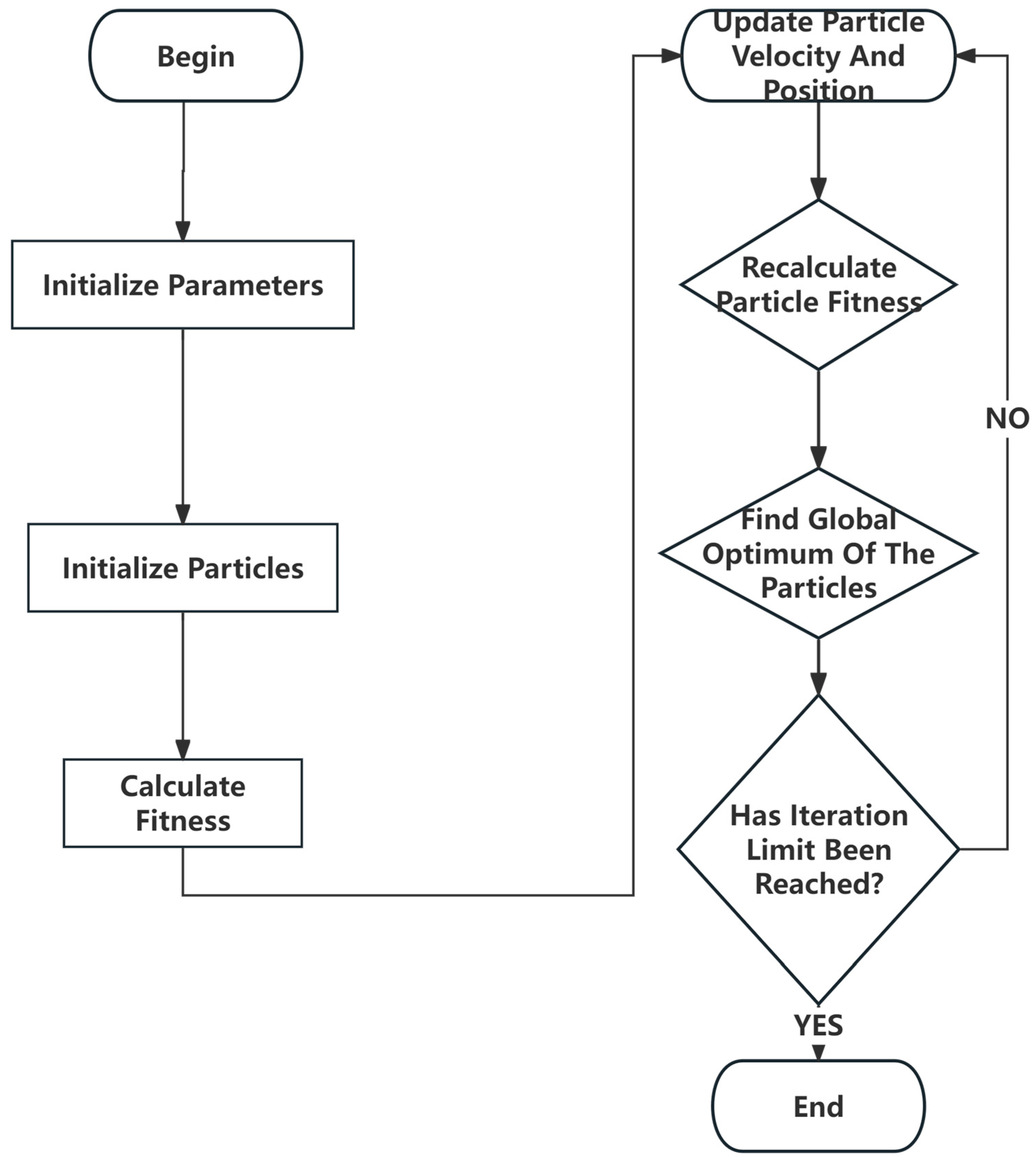
2.3. Particle Swarm Optimization (PSO) Algorithm

Particle Swarm Optimization (PSO) is an evolutionary computation technique inspired by the study of bird flock foraging behavior. The core idea of PSO is to utilize the information sharing among individuals within a group to produce an evolutionary process from disorder to order in the problem-solving space, thereby obtaining feasible solutions to the problem.

In the PSO algorithm, each particle in the search space can be regarded as a solution to the actual problem. The quality of the solution is reflected by the fitness value calculated using a fitness function; a higher fitness value indicates a closer proximity to the optimal solution. Each particle has a random initial position and velocity. Based on its individual historical best and the group’s historical best information, the particle searches for the optimal position in the space. Through continuous iteration and updates, the particle swarm is able to converge towards the global optimal position, thereby obtaining the optimal solution to the problem (for references, see acoustic emission research). The particles update their velocities and positions according to specific formulas.

$$v_i^{k+1}=\omega \times v_i^k+c_1\times r_1\times \left[x_{bes{t}^{(i)}}^k-x_i^k\right]+c_2\times r_2\times \left[x_{best}^k-x_i^k\right]$$

(2)

$$x_i^{k+1}=x_i^k+v_i^{k+1}$$

(3)

In the formula provided, $v_i^k$ and $x_i^k$ represent the velocity and position of the i-th particle during the k-th iteration, respectively. Additionally, pi(k) and g(k) denote the historical best position of the i-th particle and the global best position of the entire swarm during the k-th iteration, respectively. The inertia weight is represented by w, while c1 and c2 are the individual and social learning factors, typically ranging between [0, 2]. Both r1 and r2 are random numbers generated within the range [0, 1]. To ensure that particles conduct effective searches within a certain space during the search process, the particles’ positions and velocities need to be constrained within specific ranges, namely [−x_max, x_max] and [−v_max, v_max], respectively. These constraints help to prevent particles from straying too far from promising regions of the search space and ensure that the search remains focused and efficient.

The main implementation steps of the Particle Swarm Optimization (PSO) algorithm are outlined in the following Figure 5:

2.4. Backpropagation Neural Network

The BP (Back Propagation) neural network employs the gradient descent method for error backpropagation, adjusting weights and thresholds based on the error to achieve a desired level of accuracy. During forward propagation, signals travel through the neurons. We denote the input layer neurons as X_i, the hidden layer neurons as H_j, the activation function as f(x), the weights as ωij, and the thresholds as b_j. The actual and simulated values are represented as Y_n and y_n, respectively, while E(ω,b) is the error function with respect to the variables ω (weights) and b (thresholds).

$$H_j=f(\sum {\omega }_{ij}{x}_i+b_j)$$

(4)

$$E(\omega ,b)=\sqrt{{{\displaystyle \frac{(Yn-yn)}{n}}}^2}$$

(5)

$${\omega }_{ij}=-\eta {\displaystyle \frac{\partial E\left(\omega ,b\right)}{{\partial }_{\omega }}}$$

(6)

To evaluate the performance of a predictive model, three commonly used performance indicators are the Mean Absolute Percentage Error (MAPE), Root Mean Squared Error (RMSE), and the coefficient of determination (R²). A lower MAPE and RMSE, or an R² closer to 1, indicate a better predictive performance for the model. The formulas used to calculate these performance metrics for prediction results are as follows:

$$E_{MAP}={\displaystyle \frac{1}{n}}{\displaystyle \sum _{i=1}^n\frac{\left|Y_i-y_i\right|}{Y_i}}\times 100\%$$

(7)

$$E_{RMS}={{\displaystyle \sum _{i=1}^n\sqrt{\frac{\left(Y_i-y_i\right)}{n}}}}^2$$

(8)

$$R^2=1-{\displaystyle \frac{{{\displaystyle \sum _{i=1}^n\left(Y_i-y_i\right)}}^2}{{\displaystyle \sum _{i=1}^n{\left(Y_i-y_i\right)}^2}}}$$

(9)

In the formula, n denotes the number of data points; Y_i represents the actual value; y_i represents the predicted value; and Y⁻ (or sometimes denoted as μY or simply mean (Y)) denotes the average of the actual values.

3. Model Construction

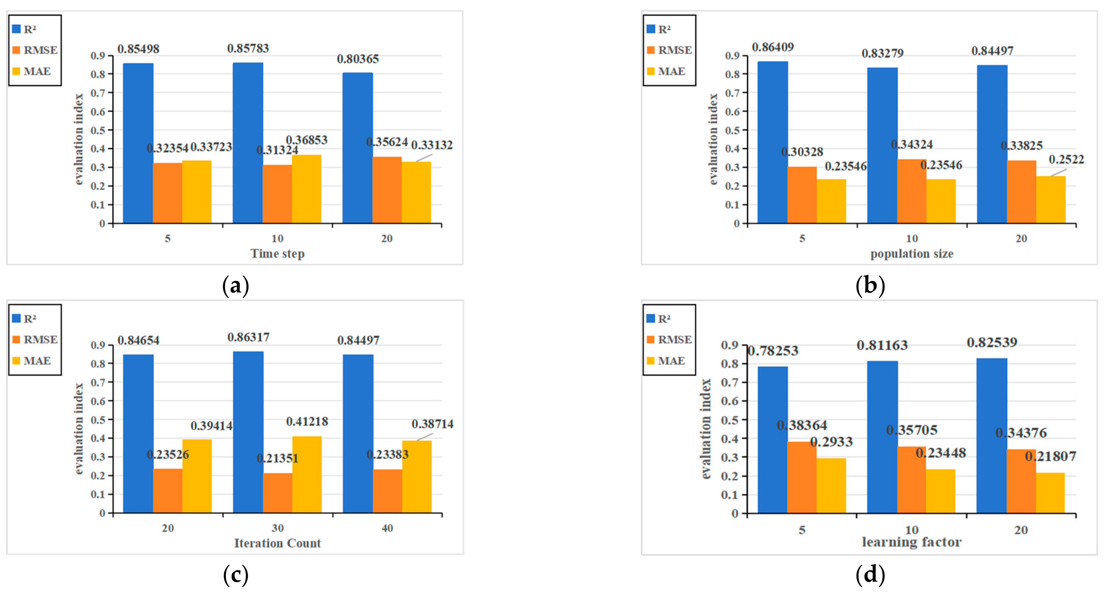
3.1. Hyperparameter Optimization

This study evaluates performance using the Root Mean Squared Error (RMSE), coefficient of determination (R²), and Mean Absolute Error (MAE) scores. Lower RMSE and MAE values indicate better predictive performance of the model. The R² value ranges from 0 to 1, with values closer to 1 indicating a better fit of the model to the data. Figure 6 presents the selection of four hyperparameters: time step, number of iterations, population size, and learning factor. The central value on the x-axis of each bar chart represents the optimal hyperparameter value used in the model. The average and minimum RMSE values for the four hyperparameters are very similar, so the R² score is used for comparison.

It is worth noting that, while RMSE and MAE provide insights into the absolute errors between predictions and actual values, R² offers a measure of how well the model’s predictions explain the variability of the actual data. By comparing R² scores, we can assess which hyperparameter configuration results in a model that best captures the underlying patterns in the data. Additionally, the similarity in RMSE values across different hyperparameter settings suggests that the model’s performance in terms of absolute error may not be highly sensitive to these specific hyperparameters within the tested range.

As shown in Figure 6a, a time step unit value of 10 yields a higher R² score. Excessively large values may lead to memory overflow and becoming stuck in local optima, while excessively small values may reduce computational efficiency. For the population size, which typically ranges from 3 to 10, smaller values can reduce the number of iterations in model training but may increase the bias in model validation accuracy. Larger values, on the other hand, increase the number of training iterations but reduce the bias in model validation accuracy. As illustrated in Figure 6b, a population size of 5 significantly improves the R² value compared to 10 and 20, making it a reasonable choice for conserving computational resources. In Figure 6c, an iteration count of 30 results in a higher R² value. As shown in Figure 6d, selecting a learning factor of 20 yields a significantly higher R² score compared to 5 and 10. Therefore, the optimal values for the four hyperparameters are determined to be 10, 5, 30, and 20, respectively.

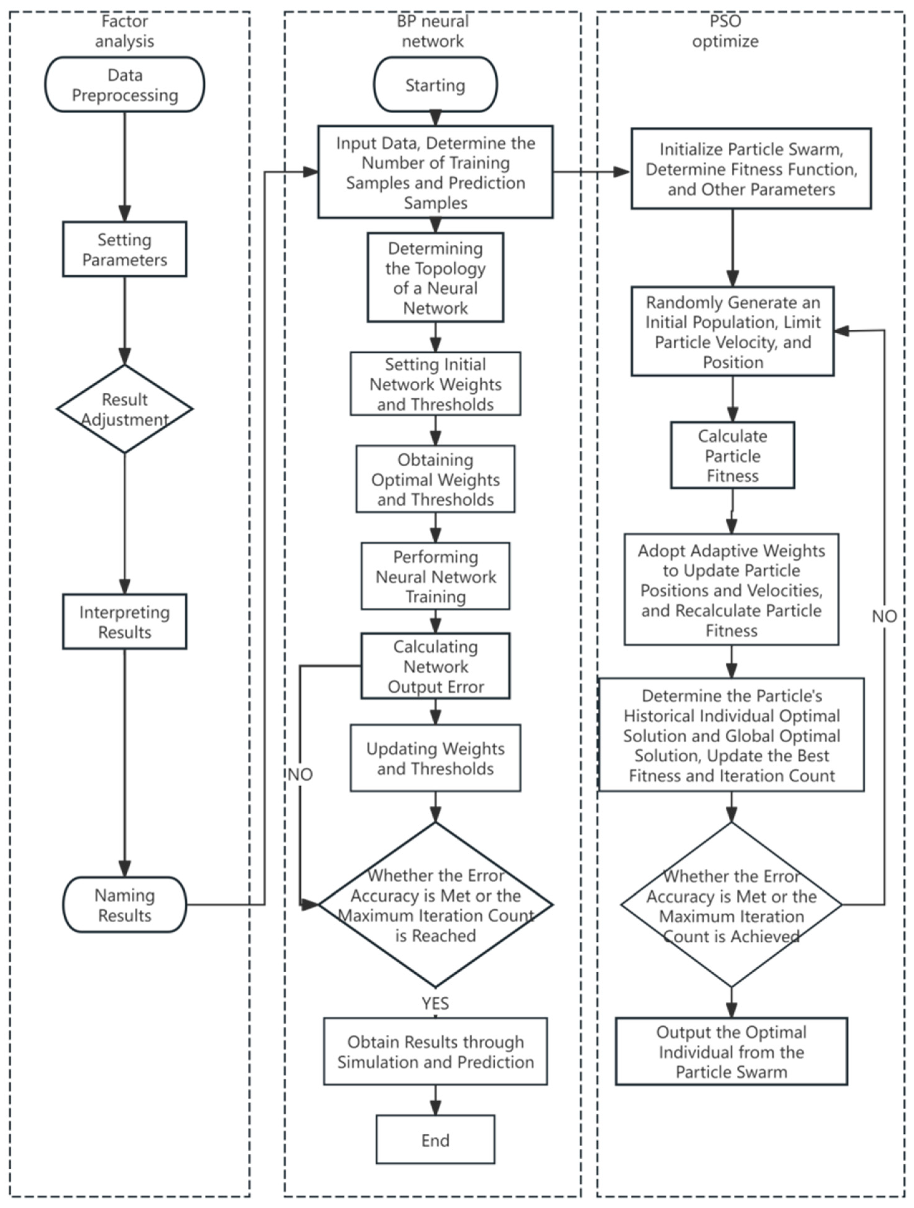
3.2. FA-PSOBP Construction of Optimized Model

The Particle Swarm Optimization (PSO) algorithm mimics evolutionary or physical processes in nature to achieve efficient search and optimization within a larger parameter space. These algorithms leverage population-based search and random selection mechanisms, allowing for the exploration of a broader range of parameter combinations and the discovery of global optimal solutions to avoid local optima. The flowchart for the FA-PSOBP prediction model is illustrated in Figure 7.

The specific process for rock mass acoustic emission prediction based on the FA-PSOBP model is as follows:

Step 1: Prepare and preprocess the dataset for model training.

Randomly divide the acoustic emission sample dataset into a 70% training set and a 30% testing set. Normalize the data for model training to ensure that it is within a suitable range for the neural network.

Step 2: Perform factor analysis and weighting.

Conduct factor analysis on 10 units to identify significant factors. Assume that the factor analysis results in 3 factors, y1, y2, and y3, which together account for 88.325% of the total variance and are considered meaningful. Perform weighting calculations on these factors to obtain a composite input for the BP neural network.

Step 3: Determine the BP neural network structure.

Define the number of neurons in the input layer and output layer. In this case, both are set to 1, as we are predicting a single output value based on a single input (the composite factor obtained from Step 2). Determine the number of hidden layer nodes. This is typically conducted using empirical formulas or through trial and error. One common formula for determining the number of hidden layer nodes (H) is

$$H={\left(R+C\right)}^{0.5}+r$$

(10)

In Equation (10), R represents the number of input layer neurons (Input Nodes) (in this study, it is 3 (corresponding to Y1, Y2, Y3)); C represents the number of output layer neurons (Output Nodes) (in this study, it is 1 (the predicted value Y)); and r represents the empirical adjustment factor (Empirical Adjustment Factor), which typically ranges from 1 to 10 (in this study, it was determined to be 3 through grid search).

Step 4: Particle Swarm Optimization (PSO) for BP Neural Network.

In this step, the initial connection weights and thresholds of the BP neural network are treated as the target parameters for optimization using the Particle Swarm Optimization (PSO) algorithm. Through the iterative process of PSO, the optimal initial connection weights and thresholds are obtained. The specific implementation steps are as follows:

Initialize PSO parameters. Set the population update iterations F = 200, population size p = 30, and individual and social learning factors c1 = c2 = 2. Initialize the particle swarm’s positions and velocities, both constrained within the range [−1,1]. The fitness function is consistent with the objective function of the BP neural network in Equation (8), which is the mean squared error of the network’s predictions, thus minimizing the network error.

Perform PSO iterative optimization. Calculate the initial fitness of the particles based on the fitness function to obtain the initial best particle. Calculate the population fitness and update the particles’ velocities and positions using Equations (2) and (3) to determine the particles’ individual best solutions and the global best solution. After iterations, all particles in the swarm will move towards the optimal solution until the minimum error accuracy is achieved or the maximum number of iterations is reached, at which point the optimal particle individual is output.

Run the BP neural network optimized by PSO. Assign the parameters corresponding to the optimal individual obtained in Step 2 to the weights and thresholds in the BP neural network net structure parameters. Then, run the neural network to train and obtain the optimal model.

Step 5: Performance Error Analysis.

Performance error analysis focuses on analyzing the prediction errors for the test set. The error metrics include the following:

Mean Absolute Error (MAE): Measures the average absolute difference between the predicted values and the actual values.

Mean Relative Error (MRE): Measures the average relative difference between the predicted values and the actual values.

Mean Squared Error (MSE): Measures the average squared difference between the predicted values and the actual values.

Root Mean Squared Error (RMSE): The square root of MSE, providing a measure of the standard deviation of the prediction errors.

$$\mathrm{MAE}={\displaystyle \frac{1}{\mathrm{n}}}{\displaystyle \sum _{i=1}^n\left|Yi-yi\right|}$$

(11)

$$\mathrm{MSE}={\displaystyle \frac{1}{n}}{\displaystyle \sum _{i=1}^n{\left(Yi-yi\right)}^2}$$

(12)

$$\mathrm{RMSE}=\sqrt{{\displaystyle \frac{1}{n}}{\displaystyle \sum _{i=1}^n{\left(Yi-yi\right)}^2}}$$

(13)

$$\mathrm{MRE}={\displaystyle \frac{1}{n}}{\displaystyle \sum _{i=1}^n\left|\frac{Yi-yi}{Yi}\right|}$$

(14)

Specifically, Y_i denotes the “actual value” for a given data point, y_i signifies the corresponding “predicted value”, and n stands for the “total number of data points”.

The linear fit assesses the degree of linear correlation between the predicted values and the actual values.

By analyzing these error metrics and the linear fit, we can evaluate the prediction accuracy and the degree of fit of the model. This helps in assessing the performance of the FA-PSOBP model in predicting rock mass acoustic emissions.

4. Result and Discussion

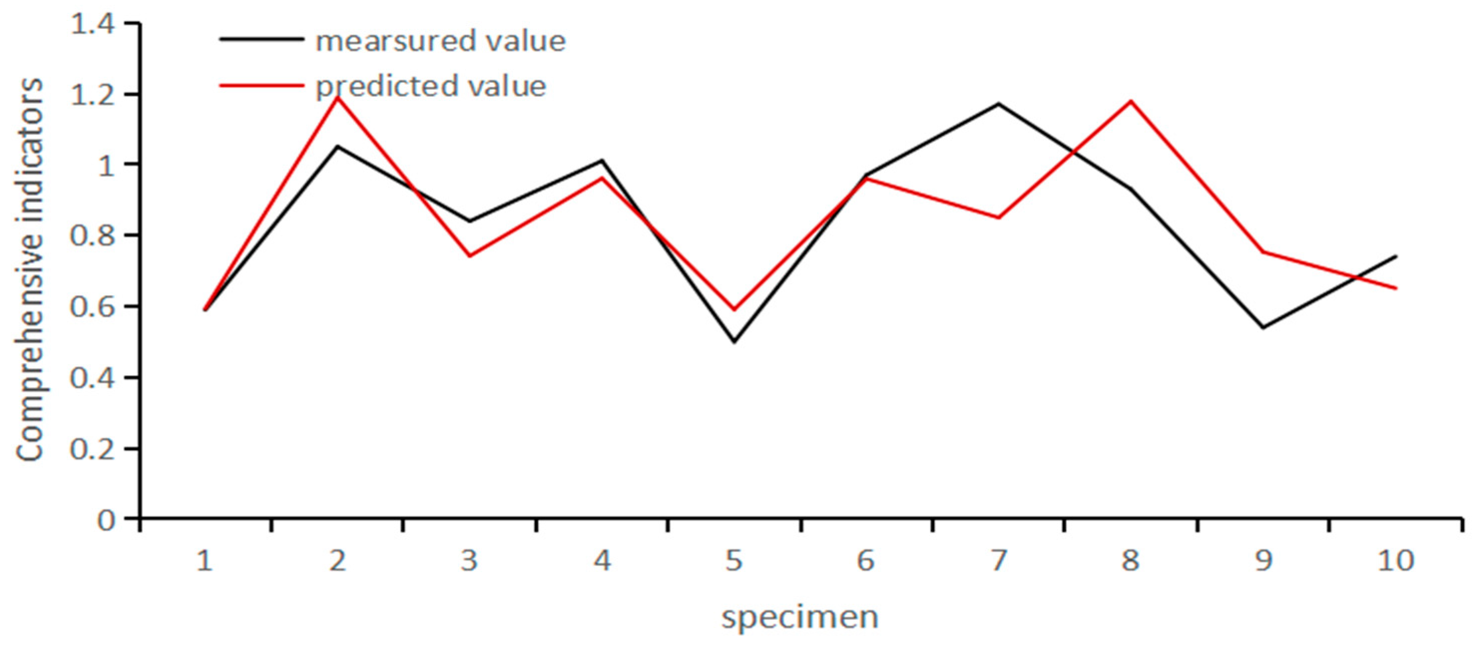
4.1. Prediction Performance Comparison

To validate the performance of the FA-PSOBP prediction model proposed by the author, simulations of the prediction model were conducted using Matlab functions and the Neural Network Toolbox. The parameter settings are as follows: the prediction time horizon length was set to 1, indicating a single-step prediction; the time step, number of iterations, population size, and learning factor were set to 10, 5, 30, and 20, respectively. The reduced dimensional acoustic emission signals collected in Section 2 were used as input samples for the acoustic emission time series prediction model. Among these, 190 sets of data were selected as training data for the prediction model, while the remaining 10 sets were used as test samples for the training, learning, and predictive analysis of the acoustic emission time series. The results are presented in

Table 4. Prediction Results Table.

Number	Comprehensive Indicator Y
	Measured Value	Predicted Value	Relative Error
191	0.59	0.593268406	0.55%
192	1.05	1.188406557	14.54%
193	0.84	0.741827053	11.61%
194	1.01	0.960578817	4.89%
195	0.5	0.59110598	18.23%
196	0.97	0.959367536	1.03%
197	1.17	0.849890528	27.35%
198	0.93	1.177363619	25.80%
199	0.54	0.652859941	20.37%
200	0.74	0.650975516	12.16%
Average Relative Error %	13.653%

and Figure 8.

The experiment utilized 200 sets of acoustic emission data which were divided into a training set (140 sets) and a test set (60 sets) in a 7:3 ratio. This division follows conventional practices in time series prediction, ensuring that the training set covers complete evolutionary cycles, while the test set focuses on the critical failure stage (the last 60 sets of data corresponding to rockburst precursors). The model was optimized for hyperparameters through 5-fold cross-validation within the training set to avoid overfitting.

The prediction errors for samples 197, 198, and 199 in Figure 8 are relatively high (27.35%, 25.80%, and 20.37%, respectively). Possible reasons for this include the following:

Data noise interference: During the stage approaching rockburst, acoustic emission signals are susceptible to interference from equipment vibration or ambient noise, leading to abnormal parameter measurements (such as sudden changes in d7-RMS voltage).

Model sensitivity: The PSO-BP model has limited capability in capturing high-frequency transient signals. Further optimization is needed, potentially through the integration of wavelet denoising techniques.

Heterogeneity of rock mass: The uneven distribution of microcracks within the samples may cause the acoustic emission response of local failure events to deviate from statistical laws.

These factors could collectively contribute to the higher prediction errors observed for these specific samples.

Simultaneously, we need to evaluate the predictive performance of the FA-PSOBP model from both vertical and horizontal perspectives. Firstly, by comparing the average accuracy of the model before and after optimization, we must analyze the impact of the PSO process on the original model to determine whether it has a positive or negative effect. To assess the optimization capability of PSO compared to other algorithms, it is necessary to conduct a comprehensive comparison of the performance of FA-PSOBP with common optimization models.

As shown in

Table 5. Performance Comparison of different machine learning models in rockburst prediction.

Title 1	R2	Mean Relative Error
FA-PSOBP	0.864	13.65%
LSTM	0.845	18.76%
CNN	0.744	21.44%
SVM	0.782	19.88%
Random Forest	0.721	23.12%

, the FA-PSOBP model outperforms the comparison models in terms of both R² and error indicators. Although LSTM and CNN perform well due to their inherent advantages in processing time series, they still suffer from relatively high errors. By utilizing factor analysis for dimensionality reduction and PSO for optimizing weights, FA-PSOBP effectively balances accuracy and efficiency, verifying its reliability as a tool for rockburst prediction.

The table reveals that the relative error of the FA-PSOBP prediction model is relatively small. To provide a more intuitive comparison of model performance, when compared to the unoptimized BP prediction model, the FA-PSOBP prediction model demonstrates better fitting between its predicted values and the target values of the training set, exhibiting higher prediction accuracy. This proves the effectiveness of the FA-PSOBP prediction model in predicting acoustic emission time series and provides a certain theoretical basis for accurate predictions.

From

Table 6. Performance comparison between FA-PSOBP and benchmark models in rockburst prediction.

Title 1	R2	Mean Relative Error
FA-PSOBP	0.864	13.65%
BP	0.714	22.27%
GA-BP	0.824	19.18%

, it can be observed that the FA-PSOBP model exhibits higher accuracy compared to other machine learning methods.

4.2. Discussion

The results of this study demonstrate that the FA-PSOBP model exhibits superior performance in predicting acoustic emission (AE) parameters compared to traditional BP and LSTM models. This improvement can be attributed to the effective integration of factor analysis (FA) and Particle Swarm Optimization (PSO), which enhances the model’s ability to handle high-dimensional data and avoid local optima. Compared to previous studies, our model achieves a higher R² value (0.86409) and a lower mean relative error (13.653%), indicating better predictive accuracy.

Notably, prior research employing machine learning for AE-based rockburst prediction has predominantly focused on classification tasks (e.g., severity levels) rather than regression-based time series forecasting. For instance:

Pu et al. [24] compared 10 machine learning methods (including SVM, BP, and RF) for microseismic event identification, achieving classification accuracies of 75–85% but did not report R² values for regression tasks. Zhang et al. [26] utilized a CNN with dynamic moving windows to predict microseismic parameter trends, reporting an R² of 0.79–0.82, which is lower than our model’s 0.864. Hu et al. [29] applied LSTM to predict microseismic information, achieving an R² of 0.83, slightly below the FA-PSOBP’s performance. Jian et al. [23] employed a Random Gradient Boosting model for rockburst classification using AE data but focused on accuracy metrics rather than regression scores.

These comparisons highlight that, while existing studies often prioritize classification, our work advances the regression-based prediction of AE parameters, offering a more granular tool for early warning systems. The FA-PSOBP’s R² surpasses both conventional models (e.g., BP neural networks at 0.714) and hybrid approaches like GA-BP (0.824), as shown in Table 6. This underscores the efficacy of factor analysis in reducing dimensionality and PSO in optimizing neural network weights, addressing key limitations in prior AE signal processing.

The implications of this research are significant for the field of rockburst early warning systems. By accurately predicting AE parameters, the FA-PSOBP model can provide timely warnings for potential rockburst events, thereby improving safety in deep underground engineering projects. This is particularly relevant in mining and tunneling operations, where rockbursts pose serious risks to personnel and equipment.

Future research could focus on further optimizing the FA-PSOBP model by incorporating additional data sources, such as microseismic monitoring or electromagnetic radiation signals. Additionally, the model could be tested on larger datasets from different geological conditions to validate its generalizability. Exploring other optimization algorithms, such as genetic algorithms or simulated annealing, may also yield further improvements in prediction accuracy.

5. Conclusions

5.1. Acoustic Emission (AE) Signal Analysis for Rockburst Prediction

The variation patterns of various characteristic parameters of acoustic emission signals can be used to infer the evolution of rock mass fracture activities and assess the stability status of rock masses. This, in turn, allows for the prediction of dynamic disasters such as rockbursts. Therefore, acoustic emission technology demonstrates certain effectiveness and feasibility in studying the processes of rock mass fracture instability and disaster evolution.

5.2. Factor Analysis for AE Time Series

To address the issue of information redundancy in rock mass fracture acoustic emission time series, a factor analysis is applied to extract the different characteristic parameters of AE signals, resulting in new comprehensive indicator parameters. By using the factor analysis algorithm to reduce the complexity of high-dimensional AE signals, not only is sample redundancy eliminated and the utilization rate of effective information improved, but also a solid foundation is laid for subsequent predictions of AE time series and accurate predictions of rockbursts.

5.3. Improved FA-PSOBP Model for AE Time Series Prediction

By modifying the connection weights of the FA-PSOBP model’s interconnected nodes, and through practical examples, it has been proven that the FA-PSOBP prediction model exhibits high prediction accuracy in forecasting acoustic emission time series. This demonstrates the model’s potential in providing reliable predictions for rockburst-related phenomena based on AE data.

In summary, acoustic emission technology combined with factor analysis and improved prediction models like FA-PSOBP offers a promising approach for monitoring and predicting rock mass stability and potential rockburst hazards.

References

1. Hoek, E.; Kaiser, P.K.; Bawden, W.F. Support of Underground Excavations in Hard Rock; Taylor and Francis, CRC Press: Boca Raton, FL, USA, 2000. [Google Scholar]
2. Wang, S.; Huang, L.; Li, X. Analysis of rockburst triggered by hard rock fragmentation using a conical pick under high uniaxial stress. Tunn. Undergr. Space Technol. 2020, 96, 103195. [Google Scholar] [CrossRef]
3. Prabhat, B.S.M.; Shakil, M.; Aibing, J. A comprehensive review of intelligent machine learning based predicting methods in long-term and short-term rock burst prediction. Tunn. Undergr. Space Technol. Inc. Trenchless Technol. Res. 2023, 142, 105434. [Google Scholar]
4. Song, Z.; Cheng, Y.; Yang, T.; Huo, R.; Wang, J.; Liu, X.; Zhou, G. Analysis of compression failure and acoustic emission characteristics of limestone under permeability-stress coupling. J. China Coal Soc. 2019, 44, 2751–2759. (In Chinese) [Google Scholar]
5. Ohtsu, M.; Grosse, C. Acoustic Emission Testing: Basics for Research-Applications in Civil Engineering; Springer: Berlin/Heidelberg, Germany, 2008. [Google Scholar]
6. Cheng, Y.; Song, Z.; Xu, Z.; Yang, T.; Tian, X. Failure mechanism and infrared radiation characteristic of hard siltstone induced by stratification effect. J. Mt. Sci. 2024, 21, 700–716. [Google Scholar] [CrossRef]
7. Glazer, S. Mine Seismology: Data Analysis and Interpretation; Springer: Cham, Switzerland, 2016. [Google Scholar]
8. Hu, X.; Su, G.; Chen, G.; Mei, S.; Feng, X.; Mei, G.; Huang, X. Experiment on Rockburst Process of Borehole and Its Acoustic Emission Characteristics. Rock Mech. Rock Eng. 2019, 52, 783–802. [Google Scholar] [CrossRef]
9. Su, G.; Shi, Y.; Feng, X.; Jiang, J.; Zhang, J.; Jiang, Q. True-Triaxial Experimental Study of the Evolutionary Features of the Acoustic Emissions and Sounds of Rockburst Processes. Rock Mech. Rock Eng. 2018, 51, 375–389. [Google Scholar] [CrossRef]
10. Mei, F.; Hu, C.; Li, P.; Zhang, J. Study on main Frequency precursor characteristics of Acoustic Emission from Deep buried Dali Rock explosion. Arab. J. Geosci. 2019, 12, 645. [Google Scholar] [CrossRef]
11. He, S.; Song, D.; Li, Z.; He, X.; Chen, J.; Li, D.; Tian, X. Precursor of Spatio-temporal Evolution Law of MS and AE Activities for Rock Burst Warning in Steeply Inclined and Extremely Thick Coal Seams Under Caving Mining Conditions. Rock Mech. Rock Eng. 2019, 52, 2415–2435. [Google Scholar] [CrossRef]
12. Li, J.; Liu, D.; He, M.; Guo, Y.; Wang, H. Experimental investigation of true triaxial unloading rockburst precursors based on critical slowing-down theory. Bull. Eng. Geol. Environ. 2023, 82, 65. [Google Scholar] [CrossRef]
13. Jia, Y.; Lu, Q.; Shang, Y. Rockburst prediction using particle swarm optimization algorithm and general regression neural network. Chin. J. Rock Mech. Eng. 2013, 32, 343–348. [Google Scholar]
14. Zhao, Z.; Gross, L. Using supervised machine learning to distinguish microseismic from noise events. In Proceedings of the SEG International Exposition and Annual Meeting, Houston, TX, USA, 24–29 September 2017; p. SEG-2017-17727697. [Google Scholar]
15. Wang, Y. Prediction of rockburst risk in coal mines based on a locally weighted C4.5 algorithm. IEEE Access 2021, 9, 15149–15155. [Google Scholar] [CrossRef]
16. Liang, W.; Sari, A.; Zhao, G.; McKinnon, S.D.; Wu, H. Short-term rockburst risk prediction using ensemble learning methods. Nat. Hazards 2020, 104, 1923–1946. [Google Scholar] [CrossRef]
17. Ke, B.; Khandelwal, M.; Asteris, P.G.; Skentou, A.D.; Mamou, A.; Armaghani, D.J. Rock-burst occurrence prediction based on optimized Naïve Bayes models. IEEE Access 2021, 9, 91347–91360. [Google Scholar] [CrossRef]
18. Wu, S.; Wu, Z.; Zhang, C. Rock burst prediction probability model based on case analysis. Tunn. Undergr. Space Technol. 2019, 93, 103069. [Google Scholar] [CrossRef]
19. Xue, Y.; Bai, C.; Qiu, D.; Kong, F.; Li, Z. Predicting rockburst with database using particle swarm optimization and extreme learning machine. Tunn. Undergr. Space Technol. 2020, 98, 103287. [Google Scholar] [CrossRef]
20. Zhili, T.; Xue, W.; Qianjun, X. Rockburst prediction based on oversampling and objective weighting method. J. Tsinghua Univ. (Sci. Technol.) 2021, 61, 543–555. [Google Scholar]
21. Papadopoulos, D.; Benardos, A. Enhancing machine learning algorithms to assess rock burst phenomena. Geotech. Geol. Eng. 2021, 39, 5787–5809. [Google Scholar] [CrossRef]
22. Yin, X.; Liu, Q.; Huang, X.; Pan, Y. Real-time prediction of rockburst intensity using an integrated CNN-Adam-BO algorithm based on microseismic data and its engineering application. Tunn. Undergr. Space Technol. 2021, 117, 104133. [Google Scholar] [CrossRef]
23. Jian, Z.; Shi, X.Z.; Huang, R.D.; Qiu, X.Y.; Chong, C. Feasibility of stochastic gradient boosting approach for predicting rockburst damage in burst-prone mines. Trans. Nonferrous Met. Soc. China 2016, 26, 1938–1945. [Google Scholar]
24. Pu, Y.; Apel, D.B.; Hall, R. Using machine learning approach for microseismic events recognition in underground excavations: Comparison of ten frequently-used models. Eng. Geol. 2020, 268, 105519. [Google Scholar] [CrossRef]
25. Ma, K.; Shen, Q.Q.; Sun, X.Y.; Ma, T.H.; Hu, J.; Tang, C.A. Rockburst prediction model using machine learning based on microseismic parameters of Qinling water conveyance tunnel. J. Cent. South Univ. 2023, 30, 289–305. [Google Scholar] [CrossRef]
26. Zhang, H.; Zeng, J.; Ma, J.; Fang, Y.; Ma, C.; Yao, Z.; Chen, Z. Time series prediction of microseismic multi-parameter related to rockburst based on deep learning. Rock Mech. Rock Eng. 2021, 54, 6299–6321. [Google Scholar] [CrossRef]
27. Di, Y.; Wang, E. Rock burst precursor electromagnetic radiation signal recognition method and early warning application based on recurrent neural networks. Rock Mech. Rock Eng. 2021, 54, 1449–1461. [Google Scholar] [CrossRef]
28. Di, Y.; Wang, E.; Li, Z.; Liu, X.; Huang, T.; Yao, J. Comprehensive early warning method of microseismic, acoustic emission, and electromagnetic radiation signals of rock burst based on deep learning. Int. J. Rock Mech. Min. Sci. 2023, 170, 105519. [Google Scholar] [CrossRef]
29. Hu, L.; Feng, X.T.; Yao, Z.B.; Zhang, W.; Niu, W.J.; Bi, X.; Feng, G.L.; Xiao, Y.X. Rockburst time warning method with blasting cycle as the unit based on microseismic information time series: A case study. Bull. Eng. Geol. Environ. 2023, 82, 121. [Google Scholar] [CrossRef]
Figure 1. Acoustic emission testing equipment.
Applsci 15 01977 g001
Figure 2. Prepare processed rock specimens.
Applsci 15 01977 g002
Figure 3. Relationship between acoustic emission parameters, time, and stress. (a) ASL, (b) RMS, (c) Initial Frequency, (d) Penk Frequency, (e) Amplitude, (f) counting, (g) energy, (h) Rising Time.
Applsci 15 01977 g003
Figure 4. The screen plot.
Applsci 15 01977 g004
Figure 5. PSO Flowchart.
Applsci 15 01977 g005
Figure 6. Hyperparameter optimization. (a) Time step, (b) Population size, (c) Iteration count, (d) Learning factor.
Applsci 15 01977 g006
Figure 7. Flowchart of the FA-PSOBP prediction model.
Applsci 15 01977 g007
Figure 8. Prediction results table.
Applsci 15 01977 g008