Article

Prototypical Graph Contrastive Learning for Recommendation

1
School of Computer Science and Artificial Intelligence, Changzhou University, Changzhou 213164, China
2
School of Microelectronics and Control Engineering, Changzhou University, Changzhou 213164, China
*
Author to whom correspondence should be addressed.
Appl. Sci. 2025, 15(4), 1961; https://doi.org/10.3390/app15041961
Submission received: 27 January 2025 / Revised: 11 February 2025 / Accepted: 11 February 2025 / Published: 13 February 2025

Abstract

:
Data sparsity caused by limited interactions makes it challenging for recommendation to accurately capture user preferences. Contrastive learning effectively alleviates this issue by enriching embedding information through the learning of diverse contrastive views. The effectiveness of contrastive learning in uncovering users’ and items’ latent preferences largely depends on the construction of data augmentation strategies. Structure and feature perturbations are commonly used augmentation strategies in graph-based contrastive learning. Since graph structure augmentation is time consuming and can disrupt interaction information, this paper proposes a novel feature augmentation contrastive learning method. This approach leverages preference prototypes to guide user and item embeddings in acquiring augmented information. By generating refined prototypes for each user and item based on existing prototypes to better approximate true preferences, it effectively alleviates the over-smoothing issue within similar preferences. To balance feature augmentation, a prototype filtering network is employed to control the flow of prototype information, ensuring consistency among different embeddings. Compared with existing prototype-based methods, ProtoRec achieves maximum gains of up to 16.8% and 20.0% in recall@k and NDCG@k on the Yelp2018, Douban-Book, and Amazon-Book datasets.

1. Introduction

Recommender systems can discover users’ preferences towards items and recommend potentially related items to users, which is an important method for alleviating the problem of information overload [1]. As user–item interaction data continue to grow, traditional shallow models such as matrix factorization (MF) [2] and collaborative filtering (CF) [3] often struggle to capture complex high-order relationships. Graph neural networks (GNNs) [4], on the other hand, address this limitation by learning collaborative information between nodes based on existing interaction graphs and leveraging multi-layer structures to explore potential relationships in higher-order neighborhoods. However, the performance of GNNs heavily relies on the quality of the interaction graph. In recommendation tasks, the quality of the interaction graph is often constrained by several factors. First, data sparsity [5] caused by the limited number of user–item interactions poses a significant challenge. Second, noise introduced by user misoperations or short-term behavioral preferences further impacts the graph’s reliability. Third, the lack of interaction records for certain long-tail items results in their under-representation. These issues not only weaken the expressive power of interaction graphs but also present substantial challenges for GNN-based recommendation methods.
To address the aforementioned issues related to data sparsity [6], contrastive learning (CL) demonstrates strong adaptability by extracting latent features from unlabeled data. It aims to optimize the distribution of the embedding space by constructing positive and negative sample pairs, bringing samples with similar features closer together while pushing dissimilar samples apart. This enhances the model’s representation capability for sparse data and further improves recommendation performance [7]. In graph-based contrastive learning, the primary methods for constructing contrastive views include structural augmentation and feature augmentation [8]. Structural augmentation is a strategy for constructing contrastive views by adding or removing nodes and edges in the user–item interaction graph [9]. Due to the large scale of the data, it is challenging to accurately remove noisy data or add effective interactions. As a result, existing structural augmentation methods typically adopt a random dropout approach. While removing noise or adding valid interactions can improve model performance to some extent, the dropout of critical nodes or edges may introduce additional noise. In more severe cases, such actions could disrupt the connectivity of the interaction graph, thereby undermining the ability of GNNs to capture high-order information. Ref. [10] indicates that various dropout strategies in graph structure have minimal impact on recommendation performance. Feature augmentation is a strategy that adds random noise or generates perturbations in the embedding space [11]. This approach modifies embeddings without altering the original graph structure to construct contrastive views. However, introducing excessive noise can make it difficult for the model to distinguish between meaningful feature information and irrelevant noise, thereby hindering its ability to preserve the core preference information of the features. Graph-based contrastive learning still faces the over-smoothing problem caused by deep graph convolution due to the application of graph neural networks on different views [12].
To address the limitations and challenges of graph-based contrastive learning in recommendation mentioned above, this paper proposes a simple yet effective method called ProtoRec, which employs prototype-based feature augmentation-guided contrastive views. ProtoRec distinguishes itself from existing methods that rely on random noise-based augmentation strategies by employing clustering methods to identify preference prototypes within the embedding space. By guiding all users and items to semantically construct potential neighborhood relationships and learning preference information, ProtoRec effectively addresses the challenge of distinguishing noise from meaningful features, thereby enhancing their latent representations [13,14,15]. Compared to existing prototypical contrastive learning approaches that utilize only a small amount of prototype information, ProtoRec refines prototype features for each user and item during training, ensuring the diversity of augmented information and preventing excessive similarity among embeddings within the same preference group. Furthermore, ProtoRec adopts a single-view propagation strategy, avoiding the over-smoothing problem caused by extensive and deep usage of graph convolution, while also reducing the overall complexity of the model. Our contributions can be concisely summarized as follows:
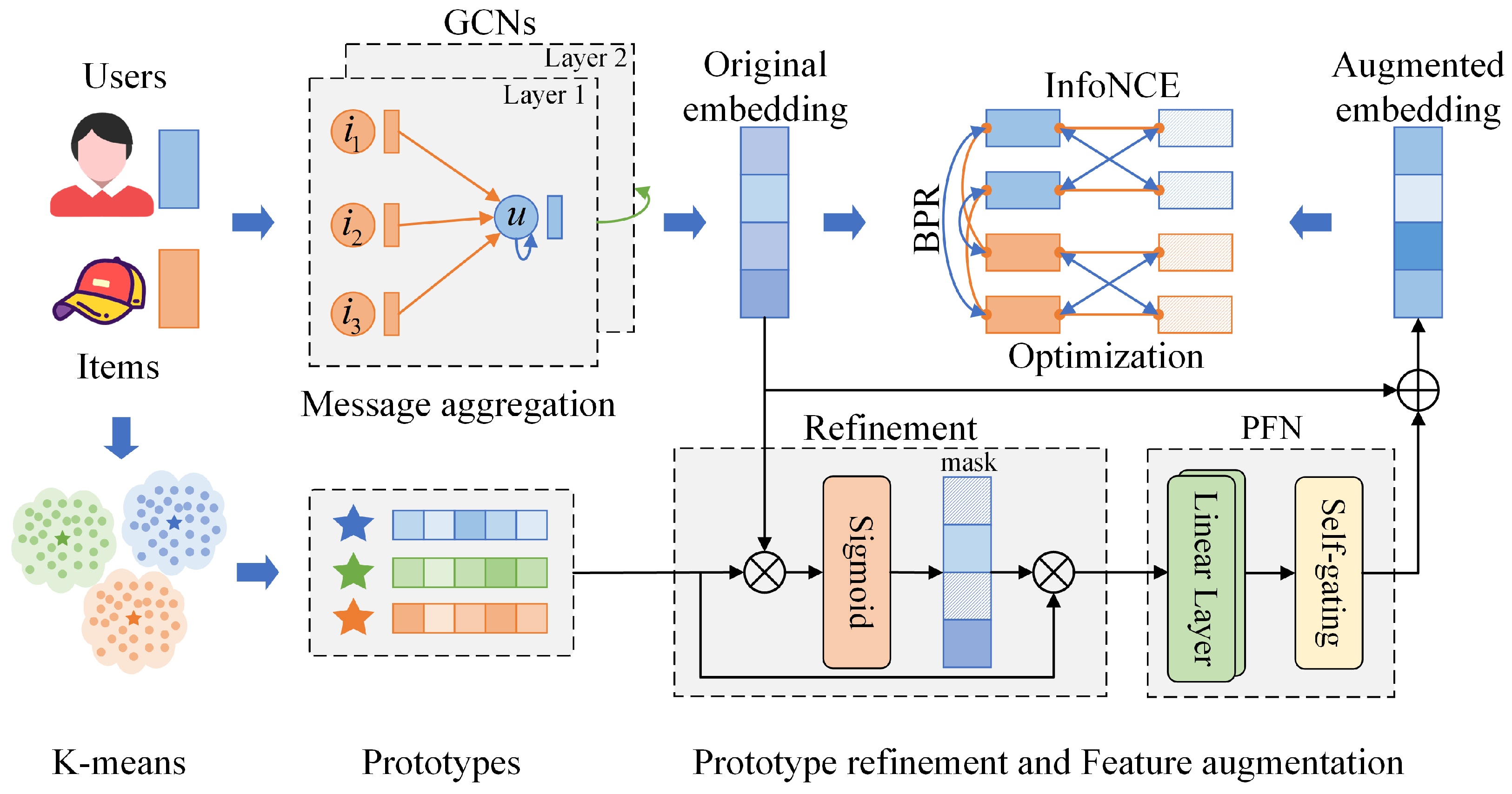
  • A novel preference prototype-based feature augmentation contrastive learning recommendation framework is proposed.
  • A preference learning module is proposed to enrich prototype information, along with a prototype filtering network to regulate feature augmentation, improving the model’s stability.
  • Compared with existing prototype-based methods, ProtoRec achieves maximum gains of up to 16.8% and 20.0% in recall@k and NDCG@k on three real-world datasets. Additional experiments were performed to further analyze the rationale behind ProtoRec.
The remainder of this paper is organized as follows: Section 2 reviews and summarizes the fundamental methods of GNNs. In Section 3, we present and analyze the proposed novel prototype-based graph contrastive learning recommendation method in detail. Section 4 conducts extensive experiments to evaluate the effectiveness of our approach in terms of recommendation performance, uniformity, ablation studies, and parameter analysis. Section 5 discusses related work from the perspectives of GNNs and CL. Finally, Section 6 concludes the paper and discusses future works.

2. Preliminaries

As a foundational method of recommender systems [4,16], graph-based collaborative filtering can recommend items to users with potential preferences based on observed feedback. Specifically, let us define a user set U = { u 1 , u 2 , . . . , u M } consisting of M users and an item set I = { i 1 , i 2 , . . . , i N } consisting of N items. To represent the observed feedback between users and items, we define the user–item interaction matrix R R M × N , where R i j = 1 denotes feedback between user u i and item v j , while R i j = 0 indicates no feedback. Then, the adjacency matrix A R ( M + N ) × ( M + N ) can be represented as
A = 0 R R T 0
In GNN-based recommendation, the initial embeddings of users and items, denoted as E ( 0 ) R ( M + N ) × d , are typically generated using the Xavier method. The exploration of latent preference between users and items based on the observed interaction graph is achieved by iteratively applying the function f p r o p a g a t e ( · ) for L layers to aggregate neighborhood information between nodes, and the function f r e a d o u t ( · ) to summarize and generate the final embedding representations. The two-stage functions for aggregating information can be specifically expressed as
E ( l ) = f p r o p a g a t e ( A ¯ , E ( l 1 ) ) E = f r e a d o u t ( [ E ( 0 ) , E ( 1 ) , . . . , E ( L ) ] )
where A ¯ = D 1 2 ( A + I ) D 1 2 represents the symmetrically normalized adjacency matrix. ( A + I ) denotes the adjacency matrix A added to the identity matrix I to achieve self-connections and maintain self-information during propagation. D is the diagonal matrix, where D i i = j ( A + I ) i j represents the non-zero instance counts in row i.

3. Methodology

In this section, the specific implementation method of ProtoRec is elaborated, detailing how ProtoRec learns graph information and the methods for prototype generation and feature augmentation. The model framework of ProtoRec is illustrated in Figure 1.

3.1. Graph Neural Network Backbone

Graph neural networks can learn neighborhood information of nodes, generating embeddings for users and items with potential preferences. They propagate node information to high-order neighborhoods through layer-wise propagation. Specifically, in ProtoRec, LightGCN [4] is adopted as the fundamental framework for the GNN module to learn the interaction information between users and items. Compared to LightGCN, ProtoRec combines the extracted prototype information to design a feature augmentation module and a single-view prototype contrastive learning method to optimize the recommendation performance of the entire model. The performance improvement of LightGCN primarily stems from its efficient aggregation of neighborhood information. As the number of propagation layers increases, the stacking of feature transformations and nonlinear activations exacerbates the over-smoothing of embeddings and significantly increases model complexity, making it unsuitable for real-time recommendation on large-scale data [4,17]. Therefore, LightGCN eliminates these two components during the aggregation process. The l-th embedding propagation layer is represented as
E ( l ) = A ¯ · E ( l 1 )
To enrich the embeddings of users and items and mitigate the impact of over-smoothing, a weighted sum function is employed to aggregate embeddings from different layers to obtain the final embedding:
E = 1 L l = 1 L E ( l )
where E R ( M + N ) × d represents the final embedding of GNN. To facilitate subsequent calculations, the embedding matrix E is split into e ( u ) R M × d and e ( i ) R N × d , representing user and item embeddings, respectively. The steps shown in Equations (3) and (4) correspond to the “GCNs” module in Figure 1. The probability prediction score y ^ u i for the interaction between user u and item i is represented in inner product form as y ^ u i = e u ( u ) T e i ( i ) . To encourage observed interaction probabilities to be higher than unobserved ones, ProtoRec employs Bayesian Personalized Ranking (BPR) [18] loss as its optimization objective. Formally, the BPR loss is represented as
L b p r = ( u , i + , i ) O log ( σ ( y ^ u i + y ^ u i ) )
where log ( · ) and σ ( · ) denote the logarithm and sigmoid functions, respectively. User u along with its corresponding positive item i + and negative item i belong to interaction set O = { ( u , i + , i ) | R u i + = 1 , R u i = 0 } . Equation (5) corresponds to the “BPR” module in Figure 1.
By optimizing the BPR loss, ProtoRec can effectively learn the neighborhood information of nodes and predict whether there is a latent preference between users and items. However, just as users in daily life often have interests in certain categories of items (electronics, cosmetics, clothing, etc.), users and items belonging to the same category are mutually associated. Next, we extract preference prototypes from embeddings of numerous users and items and construct latent neighborhood relationships.

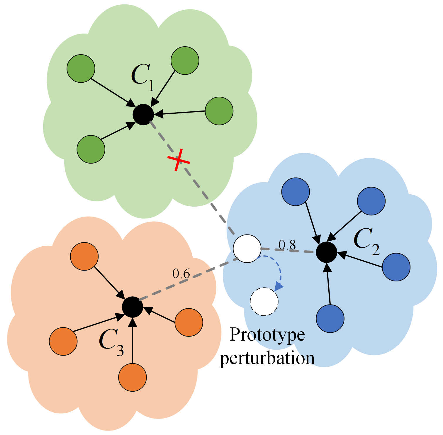
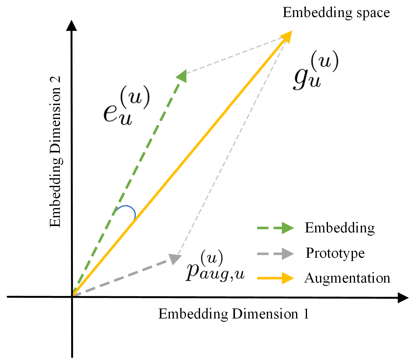
3.2. Prototype Generation and Feature Augmentation

As shown in the “K-means” module of Figure 1, to select representative preference prototypes from the dataset, ProtoRec runs the K-means clustering algorithm at each epoch to extract k cluster centers as prototypes for each category in the initialized user and item embedding spaces [19]. Although prototypes may be less accurate in the early stages of training, as the model gradually converges, the extracted prototypes progressively align with the correct clusters, ensuring feature distinctiveness while avoiding unnecessary model complexity. Unlike other methods [20,21] that extract prototypes separately for users and items, ProtoRec aims to classify all nodes with potential preferences into one category. Therefore, when implementing the K-means algorithm, users and items are considered as a whole, effectively controlling the number of prototypes. Thus, the preference prototypes proposed at each epoch are as follows:
P = k m e a n s ( E ( 0 ) )
where P R k × d represents the preference prototypes, and  k m e a n s ( · ) denotes the deployed K-means algorithm. The number of clustering centers k, serving as the basis for prototype information, is controlled through parameter tuning. In the embedding space, the clustering centers evenly partition the dataset into different categories, thereby meeting the requirements of the subsequent feature refinement module.
Although the K-means algorithm effectively extracts representative prototypes, learning the same prototype for nodes of the same class can lead to over-smoothing. As shown in Figure 2, using preference levels to measure the relationship between nodes and existing prototypes and exploring refined preferences for each user and item is an alternative method. Inspired by the self-attention mechanism, the dot product similarity E · P T between the GNN embeddings E and the prototypes P extracted by K-means is calculated as the preference scores, and a sigmoid function is deployed to normalize the preference scores. The preference scores predict the probability of the association between embeddings and prototypes, with values ranging from 0 to 1. To eliminate the influence of irrelevant prototypes, interactions with a probability below 0.5 are masked. The threshold should be set to evenly divide the probability range. Finally, the refined prototype embedding is computed by preference scores:
P r = s i g m o i d ( E · P T ) · P
where P r R ( M + N ) × d represents the refined preference prototype matrix for each user and item. Equation (7) corresponds to the “Refinement” module in Figure 1.
Due to the complexity and time-consuming nature of generating more-uniform embeddings through graph structure perturbations, ProtoRec migrates the augmentation scheme to the embedding space. In formal terms, the augmentation strategy can be represented as G = E + P r . As shown in Figure 3, taking any user u as an example, the embedding learned through the GNN is denoted as e u ( u ) , which is added to the corresponding prototype p r , u ( u ) , making the learned embedding closer to the preferred prototype and obtaining augmented embedding g u ( u ) . This can be understood as users consciously selecting their preferred categories. Since directly adding prototype information to embeddings may lead to uneven embeddings and misguide representation learning, ProtoRec employs a prototype filtering network (PFN) to balance feature augmentation. Structurally, the PFN consists of linear transformation functions f t ( · ) and f s ( · ) for enhancing model fitting, and a self-gating module f g a t e ( x ) = x · s i g m o i d ( f s ( x ) ) for controlling feature augmentation. The process of optimizing the prototype information P r through PFN and augmenting the embedding E can be represented as
G = E + f g a t e ( f t ( P r ) )
where G R ( M + N ) × d represents the final embedding after feature augmentation. Equation (8) is shown in the “PFN” module of Figure 1. For convenience, G is split into user embeddings g ( u ) and item embeddings g ( i ) . To better learn the consistency of embeddings between different augmentation views, ProtoRec employs InfoNCE [22] loss as the optimization objective for contrastive learning, which is represented as
L c l ( u ) = i B log exp ( ( e i ( u ) · g i ( u ) ) / τ ) j B exp ( ( e i ( u ) · g j ( u ) ) / τ )
where the hyperparameter τ is the temperature coefficient used to control the smoothness of the distribution. B represents the set of samples in a batch used for loss computation. exp ( · ) and log ( · ) represent the exponential function and the logarithmic function, respectively. L c l ( i ) is represented in the same way. The final CL loss is denoted as L c l = L c l ( u ) + L c l ( i ) .

3.3. Optimization

To enhance recommendation performance, ProtoRec adopts a jointly optimized strategy for the objective function:
L = L b p r + λ 1 · L c l + λ 2 · | | Θ | | 2
where Θ represents the collection of all parameters, and  λ 1 and λ 2 , respectively, denote the weight coefficients controlling the CL loss and the L 2 regularization term. The calculation process of L is shown in the “Optimization” module in Figure 1.

3.4. Algorithm Complexity

In this section, ProtoRec is decomposed into several modules to discuss complexity. Let E denote the edge numbers. M, N, and d represent user and item numbers and embedding size, respectively. In each epoch, K-means is executed to extract k prototypes with I iterations costs O ( I ( M + N ) k d ) . The complexities for constructing the interaction graph and executing L layers of LightGCN in ProtoRec are O ( 2 | E | ) and O ( 2 | E | L d ) , respectively. The time complexities for constructing the relationship graph between nodes and prototypes, as well as for reorganizing prototypes based on different weights, are O ( ( M + N ) k ) and O ( ( M + N ) k d ) , respectively. Deploying the linear transformation function in the PFN module requires O ( 2 d 2 ) . Let B and H denote the batch size and the node numbers per batch, respectively. Therefore, the time complexities for BPR loss and CL loss are O ( 2 B d ) and O ( B d + B H d ) , respectively. To better understand the training process of ProtoRec and the implementation of each module, Algorithm 1 presents the pseudocode of ProtoRec. It clearly demonstrates the execution steps of the K-means algorithm and graph-based recommendation, making it easier to comprehend the complexity of ProtoRec.
Algorithm 1 Prototypical Graph Contrastive Learning for Recommendation (ProtoRec)
1:
Input: adjacency matrix A ¯ , training dataset X , number of clusters k
2:
Output: user and item embeddings { e ( u ) , e ( i ) } for recommendation
3:
Initialize: Random initialize user and item embeddings matrix E ( 0 )
4:
while Not Convergence do
5:
    Extract k cluster prototypes P using the K-means algorithm in Equation (6)
6:
    for batch in Dataload( X ) do
7:
        Obtain user u, positive item i + , and negative item i from batch
8:
        Compute embedding E using GNNs by Equations (3) and (4)
9:
        Refine prototypes P r and augment features G using Equations (7) and (8)
10:
        Compute the total loss L by Equation (10) and back propagation
11:
    end for
12:
end while

4. Experiments

In this section, a wide range of experimental studies are conducted to validate the proposed model ProtoRec’s effectiveness in recommendation. Several key research questions are answered:
  • RQ1: How does ProtoRec perform in top-k recommendation compared to other baselines?
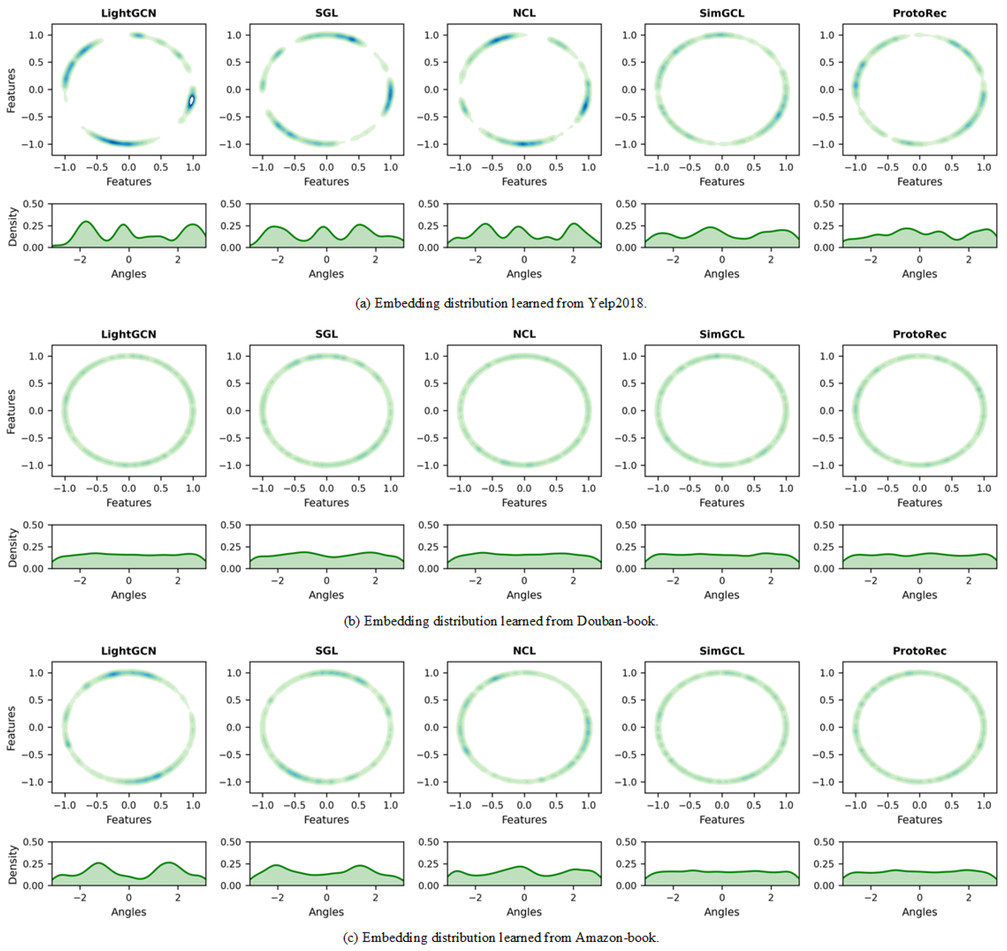
  • RQ2: How uniform are the embeddings learned by ProtoRec?
  • RQ3: How do the key components influence ProtoRec, and how is the performance of the proposed variants?
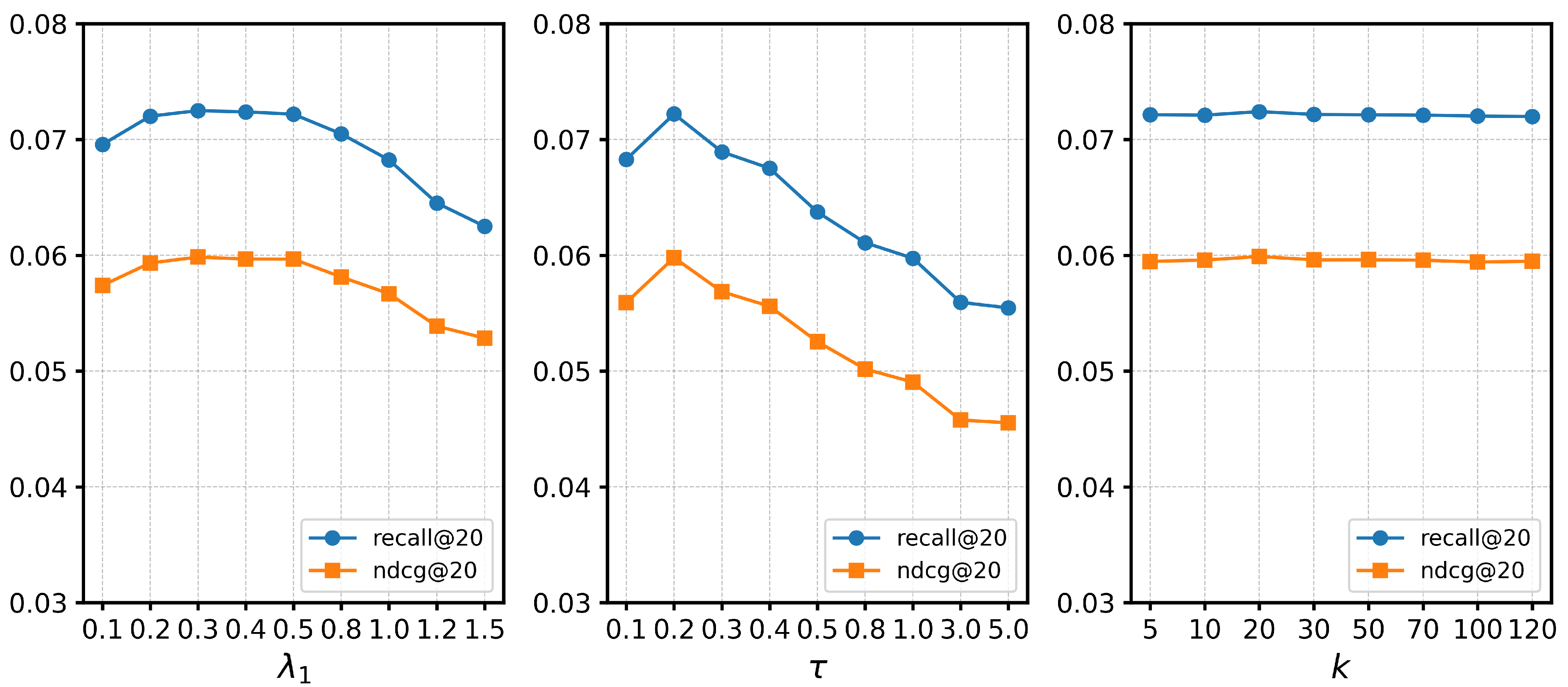
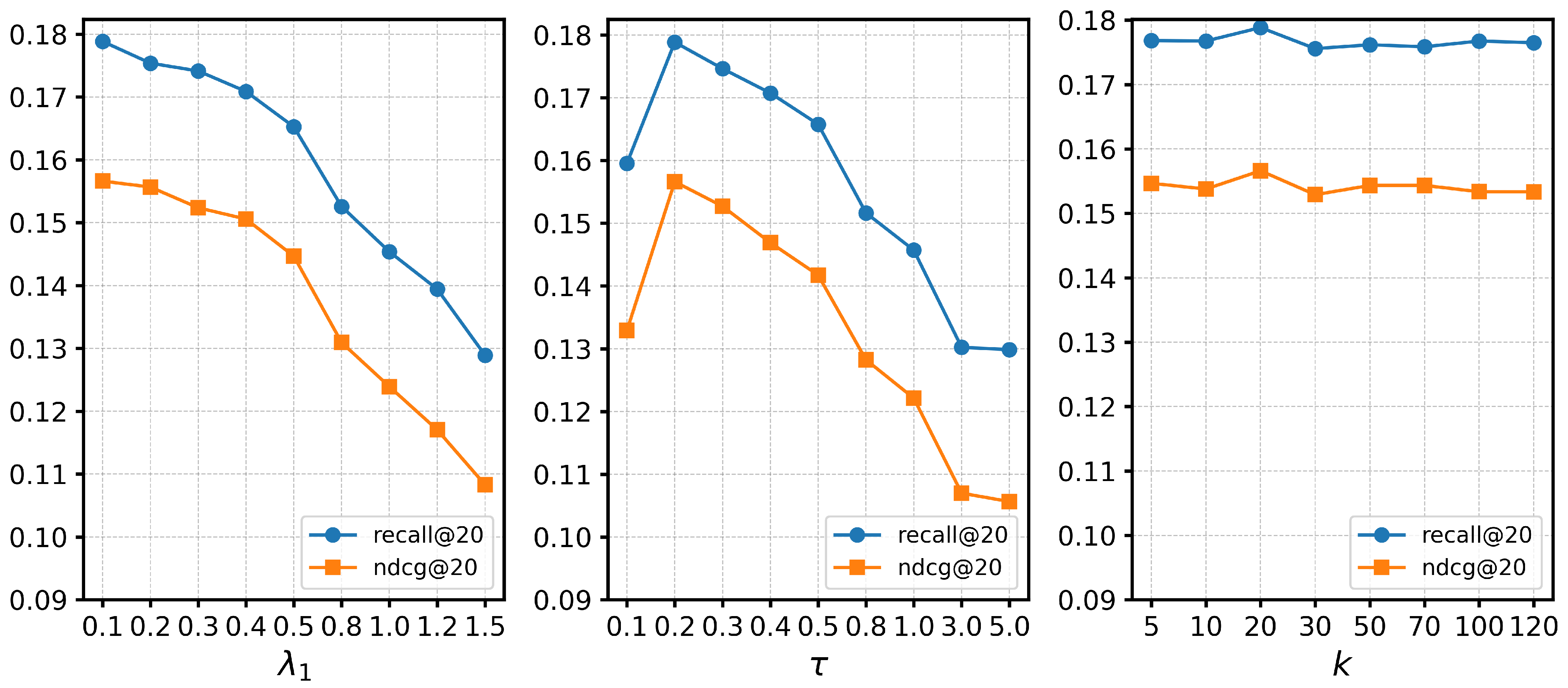
  • RQ4: How do various hyperparameter settings impact ProtoRec’s performance?
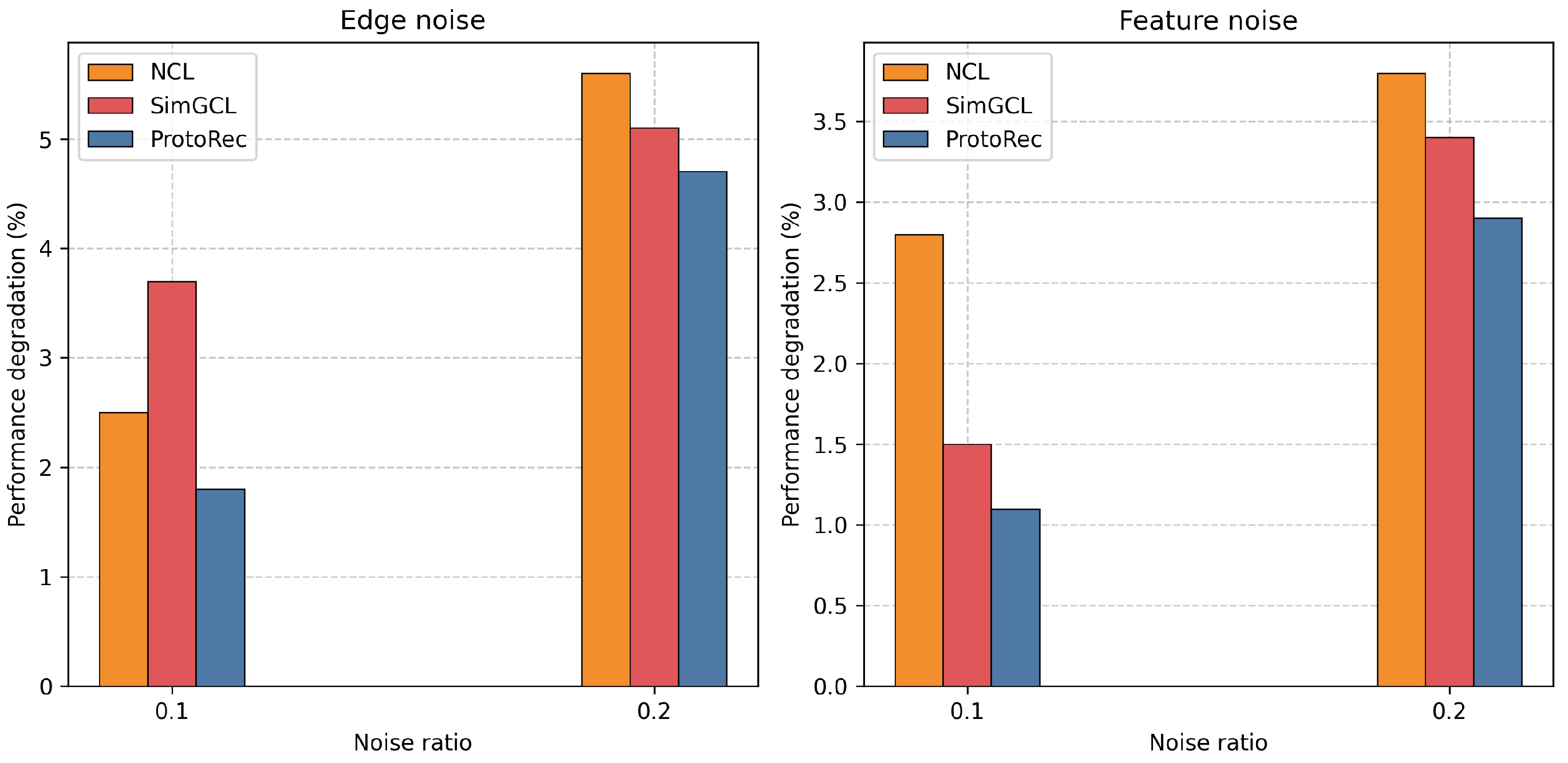
  • RQ5: How robust is ProtoRec to different types of noise?

4.1. Experimental Settings

4.1.1. Datasets and Metrics

As shown in Table 1, three real-world datasets, Yelp2018, Douban-Book, and Amazon-Book, are utilized to evaluate ProtoRec and other baseline methods. The observed interaction counts for all three datasets are very sparse, and the datasets are divided into training, validation, and test sets in a ratio of 7:1:2. To better demonstrate top-k recommendation performance, recall@k and NDCG@k are employed as evaluation metrics, where k { 20 , 40 } . Recall@k is used to measure the proportion of relevant items that are recalled in the top-k recommendations in the test set. NDCG@k further considers the ranking position of the recommendations, with higher-ranked relevant items contributing more to the metric:
R e c a l l @ k = T P @ k T P @ k + F N @ k
N D C G @ k = D C G @ k I D C G @ k
where T P and F N represent true positive and false negative, respectively. DCG and IDCG are defined as follows:
D C G @ k = i = 1 k r e l i l o g 2 ( i + 1 )
I D C G @ k = i = 1 | R E L | 1 l o g 2 ( i + 1 )
and r e l i is defined as the relevance of the i-th recommended item, typically taking a value of 0 or 1. All baseline methods were tuned using grid search within the value ranges provided in the original papers, and the training was conducted separately on each dataset to find the optimal parameter combinations.

4.1.2. Baselines

Selecting popular baselines from the corresponding fields as comparison models is involved in the construction according to ProtoRec:
  • Graph-based collaborative filtering methods.
  • LightGCN [4] is the primary choice for the graph convolutional network backbone in current recommendation models, capable of capturing collaborative information in interaction graphs in a lightweight manner.
  • DirectAU [23] optimizes embedding alignment and uniformity through a loss function and theoretically reveals the rationality of this approach for optimizing recommendation performance.
  • Self-supervised learning methods.
  • LightGCL [12] constructs perturbed views through random singular value decomposition and employs a dual-view approach for CL.
  • SGL [5] proposes random strategies to drop nodes and edges in the graph for CL.
  • SimGCL [10] introduces a feature augmentation method constructed by adding uniform noise to learned embeddings.
  • SCCF [24] decomposes the contrastive learning loss into two processes, making embeddings more compact and more dispersed, thereby enhancing the ability of contrastive learning to capture high-order connectivity information.
  • RecDCL [25] integrates batch-wise contrastive learning to enhance the robustness of representations and feature-wise contrastive learning to eliminate redundant solutions in user–item positive samples, thereby optimizing the uniformity of embeddings.
  • AdaGCL [26] dynamically reconstructs the interaction graph and denoises the data based on the learned embeddings, and it constructs contrastive learning using the embeddings learned from both processes.
  • Prototype-based recommendation methods.
  • ProtoAU [21] utilizes prototypes to optimize the alignment and uniformity of embeddings and constructs contrastive learning across different views.
  • NCL [20] constructs contrastive schemes in both semantic and structural aspects based on extracted prototypes.

4.2. Performance Comparison (RQ1)

As shown in Table 2, the performance of all baseline methods was compared across three datasets. All CL-based models outperformed LightGCN because they capture richer and more uniform embeddings by learning the consistency of embeddings from different augmented views. Similar to the objective of CL, DirectAU achieved superior performance by directly optimizing the alignment and uniformity of embeddings, surpassing some CL methods (SGL, NCL). ProtoRec’s performance was better than other prototype-based recommendation methods (ProtoAU, NCL) because it constructs feature augmented views through prototypes, enabling users and items to learn more effective preference information. The diversity of prototype information also guides more uniform distribution of embeddings. As a feature augmentation method, ProtoRec demonstrated a slight performance advantage over SimGCL while outperforming other graph structure-augmented contrastive learning methods (LightGCL, RecDCL, AdaGCL). This is likely because disrupting the integrity of interaction information can lead to insufficient training for certain nodes. Additionally, because feature augmentation does not require the extra reconstruction of large graphs, ProtoRec also achieved improvements in time efficiency. ProtoRec achieved the best performance across all three datasets, validating the effectiveness of the prototype-based feature augmentation.
When facing issues such as data sparsity and noise, LightGCN, which relies solely on graph neural network methods, requires more iterations to fit the data. In contrast, contrastive learning methods like SGL and NCL achieve more stable performance by capturing embedding diversity. DirectAU’s research on improving embedding uniformity further validates the relationship between mitigating data sparsity and enhancing embedding uniformity. LightGCL, by using a low-rank approach, can extract important information from sparse data, while methods like ProtoRec alleviate data sparsity by extracting preference prototypes that guide embedding learning of rich features. ProtoRec leverages extracted prototype information to guide users and items in learning latent preferences within the embedding space, optimizing the differentiation between positive and negative samples in contrastive learning. The application of the prototype filtering network (PFN) reduces the impact of noise, while the single-view contrastive scheme improves training efficiency, resulting in excellent recommendation performance.

4.3. Uniformity Study (RQ2)

To clearly demonstrate the uniformity of the embeddings learned by the baseline models, we used t-SNE to reduce the dimensions of 2000 randomly sampled user embeddings and plotted them in the upper half of each image. The lower half of each image shows the corresponding Gaussian kernel density estimation curves to illustrate the density estimates from different angles. As shown in Figure 4, each row is ordered based on the recommendation performance of the models. From left to right, the darker regions in the upper part of the figure decrease, and the curves in the lower part become smoother (indicating more uniformly learned features). This indicates a positive correlation between uniformity and recommendation performance. Both overly clustered and overly uniform feature distributions can hinder performance improvement.
As shown in Figure 4a,c, compared to ProtoRec and SimGCL, LightGCN, SGL, and NCL learned more clustered embedding features, with density curves exhibiting steeper trends. This phenomenon is caused by the over-smoothing issue from stacking graph convolutional networks, resulting in overly similar embeddings. Additionally, the structural perturbations in SGL make it difficult to train some nodes, also affecting the embedding distribution. As shown in Figure 4b, all baseline models learned uniform embeddings because they could effectively capture the latent relationships between users and items in the small dataset. Intuitively, ProtoRec, by guiding users and items to learn prototypes, generates clustered distributions within the same prototype, while the use of graph convolutional networks also leads to over-smoothing. However, ProtoRec alleviates the over-smoothing problem by constructing refined prototypes, guiding users and items to learn more diverse and enriched preference information. Unlike SimGCL, which adds uniform noise to the embeddings, ProtoRec purposefully directs embeddings to learn from prototypes, achieving a uniform embedding distribution.

4.4. Ablation Study (RQ3)

In this section, we present several variants of ProtoRec to evaluate their recommendation performance. As shown in Table 3, the variant ProtoReca uses the prototype-augmented embeddings for recommendation and performs contrastive learning with the embeddings learned by the first layer of the GNN, still achieving good performance. The variant ProtoRecl extends the prototype augmentation scheme to each layer of the GNN. While it achieves better performance on some metrics in the Yelp2018 dataset, it comes at the cost of increased complexity. The variant ProtoRecc replaces the Euclidean distance in the K-means algorithm with cosine similarity. Although different similarities are used to divide the clustering results and extract prototypes, good recommendation performance is still achieved. To investigate whether ProtoRec can adapt to different clustering algorithms, we replaced K-means with alternative clustering methods such as DBSCAN, hierarchical clustering, and Gaussian mixture models. The impact of these methods on the recommendation performance is shown in the table as ProtoRecdbscan, ProtoRechc, and ProtoRecgmm. Across the three datasets, these variations still demonstrate good performance compared to ProtoRec. Although different clustering methods were employed, they all successfully extracted prototype information from the embedding space. ProtoRec effectively transformed this information into useful augmentation, thereby maintaining the stability of the model.
To explore the impact of certain modules in ProtoRec on recommendation performance, we present the results of ablation studies in Table 3. w/o-SIG examines the impact of adding irrelevant information in the prototype refinement module. Performance is slightly lower than ProtoRec across the three datasets. Although the model assigns less weight to this irrelevant information during training, directly removing these connections reduces the impact of noise. w/o-PFN removes the prototype filtering network (PFN), resulting in a significant drop in recommendation performance across all datasets. This is because assigning excessive weight to the prototype information can mislead the knowledge learned by the GNN. The PFN helps maintain a balance between the knowledge acquired by the GNN and the prototype information by adjusting the weight.

4.5. Hyperparameter Analysis (RQ4)

We conducted experiments to analyze the impact of key parameters on ProtoRec to determine their optimal values. Some parameters were set according to convention in all experiments. The batch size was 2048; the embedding size was 64. The regularization coefficient λ 2 was typically set to a small value to avoid excessive penalization. Based on mainstream baseline methods and experimental tests, ProtoRec uses a value of 1 × 10 4 across different datasets to achieve the most stable training results. All parameters were adjusted using a grid search strategy. The possible value ranges for all parameters were obtained from related work, and a generally optimal value was set. The search was conducted around this value until the optimal value was found. The search stopped when the performance began to decline in a particular direction.
The impact of L. The number of graph convolutional layers L is tuned within {1, 2, 3, 4, 5}, and the performance of ProtoRec varies significantly across different layer settings. Smaller values result in underfitting, while larger values lead to over-smoothing and increased complexity. The experimental results show that the optimal values for L on the three datasets are 2, 3, and 4, respectively.
The impact of λ 1 . The parameter λ 1 is utilized to control the weight of InfoNCE on overall optimization objective. As shown in the first image of Figure 5, Figure 6 and Figure 7, λ 1 has a significant impact on recommendation performance. On large-scale datasets, ProtoRec focuses more on optimizing the CL loss, requiring a larger value for λ 1 . Conversely, on small-scale datasets, ProtoRec tends to prioritize optimizing the BPR loss, often necessitating a smaller value for λ 1 . It is recommended to search this parameter within the range of 0 to 1 with a step size of 0.1. The search process can be terminated when performance starts to decline, as there is generally only one peak optimal solution. Therefore, the optimal values of λ 1 on the Yelp2018, Douban-book, and Amazon-book datasets are 0.3, 0.1, and 1.0, respectively.
The impact of τ . The temperature coefficient τ adjusts the similarity distribution in InfoNCE. As the value of τ decreases, the distribution becomes sharper, enhancing the discriminative power of positive samples. Conversely, as the value of τ increases, the distribution becomes smoother, improving generalization ability. The impact of τ on different datasets is illustrated in the second images of Figure 5, Figure 6 and Figure 7. Both large and small values of τ can lead to a sharp decline in performance. Although the temperature coefficient τ can take on very large values, smaller values often yield the optimal solution in ProtoRec. Therefore, it is advisable to test values within the range of 0 to 1 with a step size of 0.1. A sharp performance decline is typically observed near the optimal value, and parameter tuning can be stopped when this phenomenon occurs. Hence, the optimal value across all datasets is 0.2.
The impact of k. The parameter k is used to control the prototype numbers extracted by K-means. Exceeding the appropriate number of prototypes can partition the data into clusters with overlapping features. Conversely, insufficient prototypes may impede the accurate extraction of the data’s underlying preferences. Due to ProtoRec’s strong fitting capability, smaller values of k are often sufficient to extract appropriate prototypes. The third images of Figure 5, Figure 6 and Figure 7 illustrate the impact of k values ranging from 0 to 120 on recommendation performance. The curves show a gradual decline in performance as the number of prototypes increases (even reaching several thousand), and ProtoRec becomes increasingly time-consuming. ProtoRec does not have strict requirements on the number of prototypes. During grid search, a relatively large interval can be used for exploration. It is recommended to search within the range of 0 to 120 with a step size of 20. The search can be stopped when increasing the number of prototypes no longer results in significant performance improvement. Therefore, the optimal numbers of prototypes k are around 20, 20, and 70 for the three datasets, respectively.

4.6. Robustness Study (RQ5)

To evaluate the robustness of ProtoRec under different types of data noise, we added noise to both the graph structure and embedding distributions at noise ratios of {0.1, 0.2} and conducted extensive experiments on the Yelp2018 dataset. The “noise ratio” is used to control the degree of different types of noise added. In edge noise, we randomly discard edges in the interaction graph with a probability determined by the noise ratio, simulating data sparsity. In feature noise, the noise ratio controls the intensity of uniform noise added to each dimension of the embeddings, allowing us to evaluate the model’s generalization ability. Experiments were also carried out with the baseline methods SimGCL and NCL for comparison, with the results shown in Figure 8. The performance degradation due to feature noise is lower than that caused by edge noise across all methods, indicating that adding noise to the graph structure affects the model’s ability to learn neighborhood information. As the noise ratio increases, the performance degradation becomes more apparent. ProtoRec outperforms SimGCL and NCL in all experiments, demonstrating its strong adaptability to various types of noise. The robustness of ProtoRec can be attributed to the contrastive learning framework and prototype-enhanced information, which enable it to extract users’ and items’ latent preferences from substantial noise and effectively optimize the embedding representations by leveraging the differences between positive and negative samples.

5. Related Work

5.1. Graph-Based Collaborative Filtering

Graph-based collaborative filtering outperforms traditional recommendation methods by leveraging an interaction graph to effectively represent user–item relationships and provide more reliable embeddings for neighborhood learning. Graph convolutional networks (GCNs) [27] provide a straightforward and practical approach for capturing collaborative information in complex graph structures, being the primary framework for recommendation models such as NGCF [28] and GCMC [29]. These methods based on GCNs learn neighborhood information of nodes layer by layer from interaction graphs, but face challenges related to the complexity and over-smoothing issues induced by deep convolution [30]. Similar to SGC [17], LightGCN [4] simplifies the model by removing redundant feature transformations and nonlinear activation components. Due to its lightweight and easy-to-implement nature, LightGCN replaces GCN as a recommendation framework and integrates with methods such as contrastive learning [31,32] and diffusion models [33,34] to achieve multitask objectives, providing a novel approach for subsequent research [35].

5.2. Graph Contrastive Learning for Recommendation

Contrastive learning presents a solution to the sparsity issue in recommendation by leveraging its self-supervised nature to extract features from vast amounts of unlabeled data [36,37]. Influenced by research in other domains [38], certain studies construct suitable contrastive views by perturbing the structure of interaction graphs. SGL [5] employs a random strategy to discard nodes and edges from the interaction graph, maximizing consistency among embeddings across different views. LightGCL [12] adopts a strategy of random singular value decomposition to reconstruct the adjacency matrix, effectively preserving crucial graph structural information and offering a low-rank solution for optimizing the contrastive learning paradigm. Despite the effectiveness of graph structure perturbation, it may lead to certain nodes failing to learn useful neighborhood information, thus misguiding feature learning. Therefore, some methods different from structure augmentation have started to emerge. SimGCL [10] adds uniform noise in the embedding space to achieve feature augmentation, reducing the negative effects of graph structure perturbations. AdaGCL [26] employs variational autoencoder to generate a graph during training, mitigating the influence of noisy interaction in the original graph. Nonetheless, frequent graph generation raises concerns regarding complexity.

5.3. Prototype-Based Contrastive Learning

Compared to random augmentation strategies, prototype-based contrastive learning emphasizes extracting prototype information that represents preference groups from the embeddings of learned neighborhood information. This prototype information serves as an optimization target for embedding learning, thereby improving recommendation performance. NCL [20] constructs a structural neighbor contrastive loss function using embeddings learned at different aggregation layers of the GCN. It further employs a clustering method to capture prototype information, which is then used to design a semantic neighbor contrastive loss function as an additional optimization objective. ProtoAU [21] focuses on reconstructing the interaction graph to generate contrastive views. By ensuring the uniformity and consistency of embeddings, it incorporates prototype information to further improve embedding quality. PGCL [14] optimizes the contrastive learning loss function by re-weighting the negative sample weights according to the distance between the prototypes of positive and negative samples, thereby ensuring a clear semantic distinction between them. Unlike NCL and ProtoAU, which directly use clustering results as prototype information to optimize the loss function, ProtoRec leverages a prototype refinement module to generate unique preference prototypes for each user and item based on clustering information, significantly enriching the embedding in the augmentation strategy. Moreover, instead of applying fixed weights to all data through parameter tuning as in existing methods, ProtoRec introduces a prototype filtering network that dynamically adjusts feature augmentation weights during training, further optimizing the uniformity and consistency of embeddings. ProtoRec adopts a single-view framework, reducing the frequency of graph convolution network operations, thereby significantly improving the overall efficiency of the model.

6. Conclusions

In this work, we propose ProtoRec, an efficient recommendation model based on a prototype-based graph contrastive learning scheme. By utilizing feature augmentation to guide the embedding learning of users and items, ProtoRec uncovers latent preferences, thereby achieving significant improvements in recommendation performance and embedding uniformity. Firstly, ProtoRec employs the K-means algorithm to extract latent preference prototypes for users and items. Next, ProtoRec refines the prototype information for each user and item based on the existing prototypes and their relationship weights with the users and items. Finally, ProtoRec utilizes a simple yet effective feature augmentation scheme to construct contrastive learning. The effectiveness of this method is demonstrated by the significant recommendation capabilities achieved on real-world datasets. On the Yelp2018, Douban-Book, and Amazon-Book datasets, ProtoRec achieved the best performance on the recommendation metrics recall and NDCG. Compared to other prototype contrastive learning methods, it achieved up to a 20% performance improvement and demonstrated superior robustness to noise. In future work, we will explore how to provide more accurate and valuable prototype information for recommendation models through supervised learning while developing adaptable feature augmentation strategies to mitigate potential performance degradation caused by an excessive increase in the number of prototypes.

Author Contributions

Conceptualization, C.Y.; Methodology, T.W.; Validation, Y.Z.; Data curation, Y.Z.; Writing—original draft, T.W.; Writing—review & editing, C.Y.; Visualization, T.W.; Supervision, C.Y. All authors have read and agreed to the published version of the manuscript.

Funding

This research received no external funding.

Data Availability Statement

The data presented in this study are openly available in https://github.com/HiddenWeII/ProtoRec (accessed on 8 February 2025).

Conflicts of Interest

The authors declare no conflicts of interest.

References

  1. Wu, L.; He, X.; Wang, X.; Zhang, K.; Wang, M. A survey on accuracy-oriented neural recommendation: From collaborative filtering to information-rich recommendation. IEEE Trans. Knowl. Data Eng. 2022, 35, 4425–4445. [Google Scholar] [CrossRef]
  2. Lian, J.; Zhou, X.; Zhang, F.; Chen, Z.; Xie, X.; Sun, G. xdeepfm: Combining explicit and implicit feature interactions for recommender systems. In Proceedings of the 24th ACM SIGKDD International Conference on Knowledge Discovery & Data Mining, London, UK, 19–23 August 2018; pp. 1754–1763. [Google Scholar]
  3. He, X.; Liao, L.; Zhang, H.; Nie, L.; Hu, X.; Chua, T. Neural collaborative filtering. In Proceedings of the 26th International Conference on World Wide Web, Perth, Australia, 3–7 April 2017; pp. 173–182. [Google Scholar]
  4. He, X.; Deng, K.; Wang, X.; Li, Y.; Zhang, Y.; Wang, M. Lightgcn: Simplifying and powering graph convolution network for recommendation. In Proceedings of the 43rd International ACM SIGIR Conference on Research and Development in Information Retrieval, Virtual, 25–30 July 2020; pp. 639–648. [Google Scholar]
  5. Wu, J.; Wang, X.; Feng, F.; He, X.; Chen, L.; Lian, J.; Xie, X. Self-supervised graph learning for recommendation. In Proceedings of the 44th international ACM SIGIR Conference on Research and Development in Information Retrieval, Virtual, 11–15 July 2021; pp. 726–735. [Google Scholar]
  6. Yu, J.; Yin, H.; Xia, X.; Chen, T.; Li, J.; Huang, Z. Self-supervised learning for recommender systems: A survey. IEEE Trans. Knowl. Data Eng. 2023, 36, 335–355. [Google Scholar] [CrossRef]
  7. Ren, X.; Wei, W.; Xia, L.; Huang, C. A comprehensive survey on self-supervised learning for recommendation. arXiv 2024, arXiv:2404.03354. [Google Scholar]
  8. Ding, K.; Xu, Z.; Tong, H.; Liu, H. Data augmentation for deep graph learning: A survey. ACM SIGKDD Explor. Newsl. 2022, 24, 61–77. [Google Scholar] [CrossRef]
  9. Zhu, Y.; Xu, Y.; Yu, F.; Liu, Q.; Wu, S.; Wang, L. Deep graph contrastive representation learning. arXiv 2020, arXiv:2006.04131. [Google Scholar]
  10. Yu, J.; Yin, H.; Xia, X.; Chen, T.; Cui, L.; Nguyen, Q.V.H. Are graph augmentations necessary? Simple graph contrastive learning for recommendation. In Proceedings of the 45th International ACM SIGIR Conference on Research and Development in Information Retrieval, Madrid, Spain, 11–15 July 2022; pp. 1294–1303. [Google Scholar]
  11. Xia, J.; Wu, L.; Chen, J.; Hu, B.; Li, S.Z. Simgrace: A simple framework for graph contrastive learning without data augmentation. In Proceedings of the ACM Web Conference 2022, Lyon, France, 25–29 April 2022; pp. 1070–1079. [Google Scholar]
  12. Cai, X.; Huang, C.; Xia, L.; Ren, X. LightGCL: Simple yet effective graph contrastive learning for recommendation. arXiv 2023, arXiv:2302.08191. [Google Scholar]
  13. Liu, F.; Zhao, S.; Cheng, Z.; Nie, L.; Kankanhalli, M. Cluster-based Graph Collaborative Filtering. ACM Trans. Inf. Syst. 2024, 42, 1–24. [Google Scholar] [CrossRef]
  14. Lin, S.; Liu, C.; Zhou, P.; Hu, Z.Y.; Wang, S.; Zhao, R.; Liang, X. Prototypical graph contrastive learning. IEEE Trans. Neural Netw. Learn. Syst. 2022, 35, 2747–2758. [Google Scholar] [CrossRef] [PubMed]
  15. Xu, M.; Wang, H.; Ni, B.; Guo, H.; Tang, J. Self-supervised graph-level representation learning with local and global structure. In Proceedings of the International Conference on Machine Learning, Virtual, 18–24 July 2021; pp. 11548–11558. [Google Scholar]
  16. Wang, X.; Jin, H.; Zhang, A.; He, X.; Xu, T.; Chua, T.S. Disentangled graph collaborative filtering. In Proceedings of the 43rd International ACM SIGIR Conference on Research and Development in Information Retrieval, Virtual, 25–30 July 2020; pp. 1001–1010. [Google Scholar]
  17. Wu, F.; Souza, A.; Zhang, T.; Fifty, C.; Yu, T.; Weinberger, K. Simplifying graph convolutional networks. In Proceedings of the International Conference on Machine Learning, Long Beach, CA, USA, 9–15 June 2019; pp. 6861–6871. [Google Scholar]
  18. Rendle, S.; Freudenthaler, C.; Gantner, Z.; Schmidt-Thieme, L. BPR: Bayesian personalized ranking from implicit feedback. In Proceedings of the Twenty-Fifth Conference on Uncertainty in Artificial Intelligence, Montreal, QC, Canada, 18–21 June 2009; pp. 452–461. [Google Scholar]
  19. Kuo, C.; Ma, C.; Huang, J.; Kira, Z. Featmatch: Feature-based augmentation for semi-supervised learning. In Proceedings of the Computer Vision–ECCV 2020: 16th European Conference, Glasgow, UK, 23–28 August 2020; pp. 479–495. [Google Scholar]
  20. Lin, Z.; Tian, C.; Hou, Y.; Zhao, W. Improving graph collaborative filtering with neighborhood-enriched contrastive learning. In Proceedings of the ACM Web Conference 2022, Lyon, France, 25–29 April 2022; pp. 2320–2329. [Google Scholar]
  21. Ou, Y.; Chen, L.; Pan, F.; Wu, Y. Prototypical contrastive learning through alignment and uniformity for recommendation. arXiv 2024, arXiv:2402.02079. [Google Scholar]
  22. Oord, A.V.D.; Li, Y.; Vinyals, O. Representation learning with contrastive predictive coding. arXiv 2018, arXiv:1807.03748. [Google Scholar]
  23. Wang, C.; Yu, Y.; Ma, W.; Zhang, M.; Chen, C.; Liu, Y.; Ma, S. Towards representation alignment and uniformity in collaborative filtering. In Proceedings of the 28th ACM SIGKDD Conference on Knowledge Discovery and Data Mining, Washington, DC, USA, 14–18 August 2022; pp. 1816–1825. [Google Scholar]
  24. Wu, Y.; Zhang, L.; Mo, F.; Zhu, T.; Ma, W.; Nie, J.Y. Unifying graph convolution and contrastive learning in collaborative filtering. In Proceedings of the 30th ACM SIGKDD Conference on Knowledge Discovery and Data Mining, Barcelona, Spain, 25–29 August 2024; pp. 425–3436. [Google Scholar]
  25. Zhang, D.; Geng, Y.; Gong, W.; Qi, Z.; Chen, Z.; Tang, X.; Tang, J. RecDCL: Dual Contrastive Learning for Recommendation. In Proceedings of the ACM on Web Conference 2024, Singapore, 13–17 May 2024; pp. 3655–3666. [Google Scholar]
  26. Jiang, Y.; Huang, C.; Huang, L. Adaptive graph contrastive learning for recommendation. In Proceedings of the 29th ACM SIGKDD Conference on Knowledge Discovery and Data Mining, Long Beach, CA, USA, 6–10 August 2023; pp. 4252–4261. [Google Scholar]
  27. Kipf, T.N.; Welling, M. Semi-supervised classification with graph convolutional networks. arXiv 2016, arXiv:1609.02907. [Google Scholar]
  28. Wang, X.; He, X.; Wang, M.; Feng, F.; Chua, T.S. Neural graph collaborative filtering. In Proceedings of the 42nd International ACM SIGIR Conference on Research and Development in Information Retrieval, Paris, France, 21–25 July 2019; pp. 165–174. [Google Scholar]
  29. Berg, R.V.D.; Kipf, T.N.; Welling, M. Graph convolutional matrix completion. arXiv 2017, arXiv:1706.02263. [Google Scholar]
  30. Li, G.; Muller, M.; Thabet, A.; Ghanem, B. Deepgcns: Can gcns go as deep as cnns? In Proceedings of the IEEE/CVF International Conference on Computer Vision, Seoul, Republic of Korea, 27 October–2 November 2019; pp. 9267–9276. [Google Scholar]
  31. Xia, L.; Huang, C.; Xu, Y.; Zhao, J.; Yin, D.; Huang, J. Hypergraph contrastive collaborative filtering. In Proceedings of the 45th International ACM SIGIR Conference on Research and Development in Information Retrieval, Madrid, Spain, 11–15 July 2022; pp. 70–79. [Google Scholar]
  32. Chen, M.; Huang, C.; Xia, L.; Wei, W.; Xu, Y.; Luo, R. Heterogeneous graph contrastive learning for recommendation. In Proceedings of the Sixteenth ACM International Conference on Web Search and Data Mining, Singapore, 27 February–3 March 2023; pp. 544–552. [Google Scholar]
  33. Jiang, Y.; Yang, Y.; Xia, L.; Huang, C. Diffkg: Knowledge graph diffusion model for recommendation. In Proceedings of the 17th ACM International Conference on Web Search and Data Mining, Mérida, Mexico, 4–8 March 2024; pp. 313–321. [Google Scholar]
  34. Zhu, Y.; Wang, C.; Zhang, Q.; Xiong, H. Graph Signal Diffusion Model for Collaborative Filtering. In Proceedings of the 47th International ACM SIGIR Conference on Research and Development in Information Retrieval, Washington, DC, USA, 14–18 July 2024; pp. 1380–1390. [Google Scholar]
  35. Wu, S.; Sun, F.; Zhang, W.; Xie, X.; Cui, B. Graph neural networks in recommender systems: A survey. ACM Comput. Surv. 2022, 55, 1–37. [Google Scholar] [CrossRef]
  36. Yu, J.; Yin, H.; Li, J.; Wang, Q.; Hung, N.Q.V.; Zhang, X. Self-supervised multi-channel hypergraph convolutional network for social recommendation. In Proceedings of the Web Conference 2021, Ljubljana, Slovenia, 19–23 April 2021; pp. 413–424. [Google Scholar]
  37. You, Y.; Chen, T.; Sui, Y.; Chen, T.; Wang, Z.; Shen, Y. Graph contrastive learning with augmentations. Adv. Neural Inf. Process. Syst. 2020, 33, 5812–5823. [Google Scholar]
  38. Chen, T.; Kornblith, S.; Norouzi, M.; Hinton, G. A simple framework for contrastive learning of visual representations. In Proceedings of the International Conference on Machine Learning, Online, 13–18 July 2020; pp. 1597–1607. [Google Scholar]
Figure 1. The overall model framework of ProtoRec. The (upper) part of the figure illustrates the message aggregation process of graph convolution, while the (lower) part represents the augmentation process based on prototype information.
Applsci 15 01961 g001
Figure 2. Illustration of node–prototype relationships, where users and items select relevant prototypes for feature augmentation, while irrelevant prototypes are discarded (red cross part).
Applsci 15 01961 g002
Figure 3. Illustration of prototype-based augmentation in R 2 , where the aggregation with prototypes causes the embedding to shift towards them.
Applsci 15 01961 g003
Figure 4. The embedding distribution plots for the three datasets. The upper part of each plot shows the Gaussian and kernel density estimation (KDE) in R 2 , where darker colors represent a higher density of points in the area. The lower part depicts the KDE on angles. A smooth curve indicates that the model has learned uniform features. Each row is sorted by the model performance on the corresponding dataset, allowing an observation of the relationship between embedding uniformity and recommendation performance from left to right.
Applsci 15 01961 g004
Figure 5. Hyperparameter analysis on Yelp2018.
Applsci 15 01961 g005
Figure 6. Hyperparameter analysis on Douban-book.
Applsci 15 01961 g006
Figure 7. Hyperparameter analysis on Amazon-book.
Applsci 15 01961 g007
Figure 8. Evaluating the robustness of different baseline methods on the Yelp2018 dataset under the recall@20 metric with respect to various types of noise. Edge noise is introduced by removing edges in the interaction graph. Feature noise is added to the embeddings by injecting uniform noise.
Applsci 15 01961 g008
Table 1. Detailed information about all datasets. The symbol “#” represents the total number of entities (users, items, and interactions) in the dataset.
Dataset#Users#Items#InteractionsDensity
Yelp201831,66838,0481,561,4060.00130
Douban-Book13,02422,347792,0620.00272
Amazon-Book52,46391,5992,984,1080.00062
Table 2. Performance comparison of different models.
DatasetMetricLightGCNProtoAUNCLSGLLightGCLDirectAURecDCLSCCFAdaGCLSimGCLProtoRec
Yelp2018recall@200.05920.06110.06690.06760.06840.07040.06900.07010.07100.07210.0722
ndcg@200.04820.05030.05470.05560.05610.05830.05600.05800.05850.05960.0598
recall@400.09810.10200.10970.11200.11100.11410.11220.11390.11520.11790.1188
ndcg@400.06300.06570.07090.07230.07210.07480.07330.07450.07520.07680.0773
Douban-Bookrecall@200.14850.15000.16350.17400.15740.16400.16640.17110.17130.17740.1788
ndcg@200.12480.12650.13870.15160.13710.14130.15260.15390.15420.15610.1566
recall@400.21010.21440.22640.23820.20750.21880.21830.22850.23120.24120.2431
ndcg@400.14310.14500.15710.17010.15120.15710.15780.15960.16170.17440.1750
Amazon-Bookrecall@200.03810.03910.04440.04670.04970.05030.04910.05100.05040.05150.0519
ndcg@200.02980.03090.03440.03670.03900.04010.03990.04050.04000.04110.0413
recall@400.06270.06550.07310.07610.07960.08050.07980.08070.08010.08080.0819
ndcg@400.03910.04080.04520.04780.05030.05050.05030.05060.05060.05210.0526
Table 3. Performance comparison of different variants and ablation studies.
DatasetYelp2018Douban-BookAmazon-Book
MethodRecall@20NDCG@20Recall@20NDCG@20Recall@20NDCG@20
ProtoRecdbscan0.07160.05910.17270.14820.05180.0412
ProtoRechc0.07180.05920.17320.14920.05140.0409
ProtoRecgmm0.07190.05930.17310.14860.05150.0413
ProtoReca0.06890.05680.17060.15130.04720.0374
ProtoRecl0.07230.05970.17830.15530.05160.0411
ProtoRecc0.07220.05930.17740.15440.05110.0405
w/o-SIG0.07210.05940.17540.15430.05130.0406
w/o-PFN0.06430.05300.14730.12660.04270.0343
ProtoRec0.07220.05980.17880.15660.05190.0413
Disclaimer/Publisher’s Note: The statements, opinions and data contained in all publications are solely those of the individual author(s) and contributor(s) and not of MDPI and/or the editor(s). MDPI and/or the editor(s) disclaim responsibility for any injury to people or property resulting from any ideas, methods, instructions or products referred to in the content.

