1. Introduction
When an outbreak occurs and no vaccine is available, non-pharmaceutical interventions such as school closure or mobility reduction are crucial to lessen the transmission rate and prevent the spread of the virus. While reducing the transmission rate, achieved with a reduction in the average number of close contacts, is effective for disease eradication, it might negatively affect the economy and people’s mental health, as happened during the Coronavirus Disease 2019 (COVID-19) epidemic [
1,
2,
3,
4,
5]. Finding a balance between controlling the disease spread and minimizing these negative impacts requires a precise understanding of the transmission rate dynamics. Therefore, accurate estimation and characterization of the transmission rate are essential for optimizing control inputs. Furthermore, the importance of state estimation cannot be overstated, as it gives a more precise understanding of the system’s dynamics, facilitating more effective intervention strategies. With a transmission rate and state estimation, policymakers can implement interventions that not only reduce transmission but also minimize broader societal consequences.
The most commonly used epidemic models are based on the framework developed in [
6]. This model is described by a nonlinear dynamical system, where the state variables represent different subpopulations: susceptible, infected, and recovered. Hence, it is named the SIR epidemic model. Since then, more complex models have been developed depending on diseases and societal characteristics such as models incorporating age groups [
7,
8,
9], geographical divisions [
10,
11,
12], and more. In contrast to black-box models, these are grounded in physical principles, so their solutions have clear physical interpretations, aiding in the understanding of epidemic dynamics, disease spread, and control strategies. Moreover, since these models explicitly depend on the transmission rate, they can be used to estimate its value.
Various approaches to estimating the transmission rate have been developed. Using a deterministic SIR model and prior knowledge of infected individuals, explicit equations for the time-varying rate can be derived [
13,
14]. Additionally, least squares and functional minimization methods have been widely applied for parameter estimation [
15,
16,
17,
18]. However, these methods typically require knowledge of the initial state and transmission rate values, which are often unavailable in real-world scenarios. Observer theory offers a promising alternative since it considers available data to reconstruct unknown states and parameters. Recent studies have explored the use of observers [
19,
20] or transformed epidemic models into simpler forms to facilitate observer-based estimations [
21,
22]. However, these approaches assume that the number of infected individuals or newly infected cases is known, whereas such data are often unavailable, as shown in
Table 1, as with the COVID-19 epidemic data. Furthermore, they primarily focus on estimating a constant transmission rate, even though it can vary over time, for instance, due to seasonal effects. This limitation suggests that while observer theory is a valuable tool, its application in current studies may not be fully suitable due to the lack of appropriate data.
To address this problem, this paper proposes different methods for estimating the state and time-varying transmission rates based on the most commonly available data. Specifically, we develop a susceptible, infected, hospitalized, and immunized (SIHR) epidemic model and solve the observer problem for three different scenarios:
- (i)
Both new hospital admissions and new deaths are available.
- (ii)
Only new hospital admissions are available.
- (iii)
Only new deaths are available.
In the first case, an exponential observer is designed to estimate the susceptible subpopulation, while an explicit equation is used to estimate the transmission rate. In the second case, following the methodologies in [
22,
23,
24,
25,
26], the epidemic model is transformed into an observer canonical form using output injection and output diffeomorphism. Then, the adaptive observer described in [
27,
28] is applied. In the third case, an explicit equation is derived to estimate new hospital admissions, enabling the use of the previously developed methods.
The proposed approaches are validated through a theoretical framework and numerical simulations, demonstrating their performance across different scenarios. The solutions developed for the first and third cases successfully estimate both the states and the time-varying transmission rate. In the second case, the proposed observer provides a bounded region where the true values lie. Although these bounds are generally informative, the method fails to accurately estimate the bounds for one of the state variables.
A key advantage of these methods over the previously discussed approaches is that they rely on commonly available data, ensuring their applicability, and they do not require prior knowledge of initial values for the unknown states and parameters. Although numerical simulations generally yield good results, these methods require a convergence period (i.e., time to produce estimates that closely match real values), which can be a drawback in situations with short time-period data, such as at the onset of a pandemic.
Due to the big impact of COVID-19 and its durability over time, many countries have gathered large datasets regarding the epidemic (e.g., the UK collected data from 2020 to 2023; see
Table 1 for details on data sources). The availability of such datasets ensures the convergence of estimated values, making these methods well suited for estimating the transmission rate during the COVID-19 epidemic. In the
Section 8, transmission rate estimation methods are proposed for application to data regarding COVID-19. Furthermore, a hypothetical insight into their implications for control is given.
Table 1.
Some countries’ data availability. A tick (✓) denotes available data, whereas a cross (×) denotes unavailable data. The cross mark in some cells does not imply that those datasets do not exist; rather, it indicates that they do not appear in the cited sources.
Table 1.
Some countries’ data availability. A tick (✓) denotes available data, whereas a cross (×) denotes unavailable data. The cross mark in some cells does not imply that those datasets do not exist; rather, it indicates that they do not appear in the cited sources.
| | Data Availability | |
|---|
|
Country
|
Positive
Tests
|
New Hospital
Admissions
|
Hospitalized
Patients
|
New
Deaths
|
Vaccination
|
Source
|
|---|
| UK | ✓ | ✓ | ✓ | ✓ | ✓ | [29,30] |
| Netherlands | × | ✓ | × | ✓ | ✓ | [31,32,33] |
| France | ✓ | ✓ | ✓ | ✓ | ✓ | [34] |
| Belgium | ✓ | ✓ | ✓ | ✓ | ✓ | [35] |
| Spain | ✓ | × | ✓ | ✓ | ✓ | [33,36] |
| Italy | ✓ | × | ✓ | ✓ | ✓ | [33,37] |
The rest of this work is organized as follows:
Section 2 presents the epidemic model. In
Section 3, two outputs are considered, namely new hospital admissions and new deaths, and an exponential observer and an explicit equation, from which the unknown states and the transmission rate are estimated, are presented. In
Section 4, with the output new hospital admissions, a diffeomorphism is applied to the dynamical system so the observer canonical form is obtained, and the joint parameter and state estimation problem is solved. In
Section 5, where only data regarding new deaths are assumed to be accessible, the number of new hospitalized people is inferred by an explicit equation, allowing the usage of any of the methods developed in
Section 3 and
Section 4.
Section 6 illustrates the numerical simulations carried out.
Section 7 presents an overview of theoretical and simulation results. Finally, concluding remarks and a discussion of future directions are given in
Section 8.
Notation
Let the function
be defined as
Given a vector
, the notation
refers to the
i-th component of the vector, that is, if
v is defined as
then
for all
.
2. Problem Statement
In this section, the nonlinear dynamical system for the SIHR epidemic model with vaccination is proposed. With some basic assumptions regarding parameters and initial conditions (non-negativeness, input bounds, etc.), the system solution’s well-posedness is ensured. Then, the dynamical system is normalized and the vector notation is given. Note that the normalized system in vector notation will be used throughout the following sections.
Consider the following SIHR epidemic model:
where the state variables
,
,
, and
stand for susceptible, infected, hospitalized, and immunized subpopulations, respectively. From the sum of the equations in (
3), the dynamical equation for the total population
is obtained:
The parameters involved in (
3) are the following ones:
(immunity rate),
(natural death rate),
(infected people recovery rate),
(hospitalized people recovery rate),
(hospitalization rate), and
(disease death rate). These parameters determine the amount of people being introduced and removed from each subpopulation. Additionally, the variable
stands for the number of newborns per day that are introduced in the susceptible subpopulation (i.e., it is assumed that newborns are healthy, but they do not hold any immunity against the disease), and the known input
(vaccinated people per day), determines the amount of people moving from the susceptible subpopulation to the immunized subpopulation. Vaccines are assumed to be administered to the susceptible subpopulation for two main reasons:
(i) during the COVID-19 epidemic, vaccines were not provided to infected or hospitalized individuals; and
(ii) those who had previously been infected or hospitalized generally had to wait until their immunity waned, at which point they transitioned from the immunized to the susceptible subpopulation. The time-varying transmission rate
, which is equal to the contact rate multiplied by the probability of being infected after close contact, plays a fundamental role in the spread of any disease, that is, given the epidemic model (
3), an increase (decrease) of
implies an increment (diminution) in the appearance of new infected people. Hence, estimating
is important. Note that estimating
implies estimating the contact rate as a consequence of the proportionality between both variables.
Assumption 1 (known parameter positivity)
. Let the parameters μ, , , σ, α and ρ fulfill the condition Assumption 2 (unknown variable boundedness)
. Let the unknown time-varying transmission rate fulfill the following conditions:
- (i)
It is bounded by the non-negative and known parameters and ;where . - (ii)
It is continuously differentiable with respect to time with a bounded time derivative;
Note that throughout this paper, denotes a non-negative real number (i.e., ).
Remark 1. Since the transmission rate is proportional to the number of contact rates, as long as the contact rate is positive and bounded (i.e., in real life, it is not possible to have negative nor infinite contacts per day), and the probability of being infected is also positive and bounded, the transmission rate is also positive and bounded.
Remark 2. The contact rate is given by the average number of people that a person meets during the day. Therefore, any self-driven population will not have abrupt changes in the contact rate, and consequently, the transmission rate can be considered continuously differentiable in t. Even if abrupt and global policies affecting everybody equally are considered, which could cause a piecewise continuously differentiable transmission rate, people’s self-awareness would have already changed the contact rate (e.g., before governments apply a lockdown, people’s fear of disease would have decreased in value). So the assumption of a continuously differentiable transmission rate is still valid.
Assumption 3 (input variables)
. Regarding the input variables, the following conditions are fulfilled:
- (i)
The input variables and are continuous on .
- (ii)
Vaccination must be non-negative and it must be lesser than the sum of the susceptible subpopulation () and the new susceptible population (); .
- (iii)
The number of newborns is bounded and has positive values: .
- (iv)
The normalized newborns per day are assumed to be approximately constant.
Assumption 4 (initial conditions)
. Let the initial conditions fulfill the following conditions:where Proposition 1. Under Assumptions 1–4, the following statements hold:
- (i)
The solution for the susceptible subpopulation will be positive: .
- (ii)
The solution for all subpopulations but susceptible will be non-negative: , where .
Proposition 2 (Positively Invariant Region)
. Under Assumptions 1–3, the setwhere is positively invariant with respect to the dynamical system (3); for any , then for all . Considering Assumption 3, point
(iv), the normalized model (i.e.,
,
,
, and
) is given by the following set of equations:
where
. This change in notation (i.e.,
) has been considered for two main reasons:
(i) in the background literature,
is usually referred to as the parameter to be estimated;
(ii) considering that the estimation
is obtained from the model (
8), then
will be computed from the expression
whose value will be more reliable since the bounds for the transmission rate (see Assumption 2) are being taken into account. Recall that sat() is defined in the Notation section, Equation (
1).
Considering that
one can eliminate one of the equations (e.g.,
) and rewrite system (
8) in vector notation, that is,
where
and
,
, and
for
,
and
Two outputs will be considered from the dynamical system (
12), that is,
where
and
stand for new hospital admissions and new deaths, respectively.
For notation convenience, from now on, the time dependency of variables and functions will not be explicitly written in proofs unless it is necessary to avoid any confusion.
3. Parameter Estimation with Two Outputs
In this section, the outputs and are considered. Then, an exponential observer for the estimation of the state variable is proposed in Theorem 1 and its proof is provided. Then, the exponential convergence of the estimated is guaranteed in Proposition 3.
Considering that the outputs
and
are available, an exponential observer for the dynamical system
in (
11) and (
12) can be calculated from the solution of an auxiliary ODE, as stated in the subsequent Theorem 1 and its proof.
Theorem 1. Under Assumptions 1–4, and considering the outputs and , if for all and some , given the solution of the dynamical equationthe functionwhere ϵ refers to a positive and small value, and is an exponential observer for the dynamical equation Proof of Theorem 1. Let us define
, whose time derivative yields
Defining the error as
, its time derivative gives
whose solution verifies
Then, considering the condition
, where
L is positive, it follows that
From the definition of
z and considering that
, the expression
(equivalently
) is obtained, so
Thus, the condition for an exponential observer is verified.
Note that the function has been applied to the expression since ; see Proposition 1, where stands for a positive and small value.
□
Remark 3. The upper and lower bounds established for L are essential to ensure the exponential observer and fulfill the positivity of subpopulations, that is, by considering the expression given in (21), the conditions and ensure the exponential convergence of ; see Equation (22). From the inequality , the conditionis obtained, and the non-negativity of (see Proposition 1) leads to . Hence, the condition established in Theorem 2 is satisfied. Additionally, if , the condition (24) is satisfied for any and all . At this point, note that all the state variables are known so an explicit expression for
in terms of those variables can be obtained from the equations in (
11) and (
12). By doing this, the following result is obtained.
Proposition 3. Under Assumptions 1–4, and considering the outputs and , and obtained from (17), if for all and some , the functionwith , is an exponential estimation for the time-varying transmission rate . Proof of Proposition 3. By isolating
from the dynamical equation for
in (
11) and (
12), one obtains that
and considering
(see expression (
17)), the error
is given by the equation
The relation between
and
given in (
9) leads to
so that
With
(or equivalently
), and considering
and
(see Proposition 1), and the expression (
17) for
, respectively, it follows that
where
M is positive and bounded. Thus,
which verifies that the expression given in (
25) is an exponential estimation for
. □
4. Parameter Estimation with One Output (New Hospitalizations)
In this section, the output
is assumed to be the only available data. No linear combination has been found that transforms the nonlinear dynamical system (
11) and (
12) into a state-affine canonical form. If such a transformation existed, the problem would be simplified and could be solved, as demonstrated in the proof of Theorem 1 in
Section 3.
In the absence of such a transformation,
Section 4.1 introduces a diffeomorphism by output injection and output diffeomorphism to transform the nonlinear dynamical system (
11) and (
12) into the observer canonical form; see Theorem 2. Then, assuming that the parameter to be estimated varies slowly over time,
Section 4.2 presents an adaptive observer for the estimation of both the unknown states and the transmission rate; see Theorem 3.
As a result of the approximations made in the diffeomorphism design (see Assumption 5 for details), the estimation errors do not converge to zero but remain bounded. In
Section 4.3, additional information regarding the errors is assumed to be available, enabling the calculation of the estimation error bounds. Consequently, by considering both the estimates provided by the adaptive observer and the associated error margins, regions where the true value will lie can be determined.
4.1. Observer Canonical Form with Output Injection and Output Diffeomorphism
In this subsection, with the diffeomorphism proposed in Theorem 2, the dynamical systems (
11) and (
12) are transformed into the observer canonical form. Note that this transformation is only viable if one assumes that the term
, where
, is small enough so its effects are negligible in system (
12).
Assumption 5. Let the parameter θ be constant and the term , and for be negligible enough such that in (12) can be approximated as In this context, the conditions for the existence of diffeomorphism that transforms the nonlinear dynamical system into the observer canonical form given in [
25,
26] are fulfilled, so the steps to obtain such a change of variables have been followed. This leads to the diffeomorphism shown in the subsequent Theorem 2.
Theorem 2. Under Assumption 5, the change of coordinateswhere and , is a local diffeomorphism which transforms the system (32) into the observer canonical formwith a state vector , and Proof of Theorem 2. The inverse function of
T is given by the expression
Then, it is straightforward that for each , and for each . Thus, the function is bijective.
The Jacobian matrix of the function
leads to
whose terms exist and are continuous on
. Regarding the inverse function
, it follows that
whose terms also exist and are continuous on
. Since the function
has been proven to be bijective, and
and
are continuously differentiable on their domain, the map
is a diffeomorphism.
Differentiating
z with respect to time, where
, leads directly to the expression (
34), that is,
Then, the time derivative of the term
gives
Since
, expressions like
are well defined through the proof, so the difference between
and
, which leads to
is well defined, and the expression for
in (
34) is obtained by isolating
from the expression (
41). Finally, differentiating
with respect to time yields
and, by calculating
and isolating
, one obtains that
Thus, by substituting
with
into the expressions (
39), (
41) and (
43), the observer canonical form (
34) is obtained. □
Remark 4. Assuming that at , where , the case occurs, hospitalized people, if any, will disappear at any , and susceptible people will not be infected anymore since the infected subpopulation does not exist, so will be perpetuated for all . Therefore, this refers to a situation where the disease becomes extinct, and for this reason, the diffeomorphism is well defined over the set U, and it does not apply to cases where .
The requisites for the existence of a diffeomorphism that transforms (
11) and (
12) into (
34) can be used in two different ways depending on whether the inputs are user-defined. For inputs that are not user-defined, such as those in the dynamical system (
11) and (
12), the next step is to verify whether the conditions for the existence of the diffeomorphism are met. In contrast, in cases where the inputs can be defined, they can be chosen in a way that ensures the existence of the diffeomorphism.
Specifically, when the transmission rate
in (
11) and (
12) is considered as an input, the diffeomorphism remains valid under the assumption
. However, if
does not satisfy the condition condition (i.e.,
), a time-varying function for
can be assigned for the existence of the diffeomorphism. These results are formalized in Corollary 1.
Corollary 1. Under Assumption 5, the change of coordinates (33) transforms the system (32) into the observer canonical form (34) for a time-dependent whose variations with respect to time are small enough to assume thatwhere is given in (35), or a time-dependent transmission rate with the formfor any , where The proof of Corollary (1) follows directly from the following steps:
(i) substituting
with
in expression (
32), and maintaining
in (
33);
(ii) differentiating with respect to time the change of variables given by the expression (
33), as seen in the proof of Theorem 2. Furthermore, from the point
(i) in Proposition 1, it follows that
, so the function
given in (
45) is defined and well defined on the domain
.
4.2. Adaptive Observer
With the nonlinear dynamical system (
11) and (
12) transformed into the observer canonical form (
34) and (
35), the state variables and the parameter estimation problem will be solved with the adaptive observer proposed in [
28], which is given in Theorem 3 of this subsection. Assuming that the terms
, where
, and
are small enough, this observer is characterized by global exponential convergence.
Since we are interested in identifying the parameter
, let us rewrite the dynamical system (
34) and (
35) in a more appropriate form, that is,
where
Regarding , its dependence with respect to the known signals can simply be considered as a dependence of the time t. So, for the sake of simplicity, we will use instead of .
Now, we will recall some important points for the application of the adaptive observer in [
28]. Note that those assumptions and corollaries in [
28] have been adapted for our particular case.
Assumption 6. Assume a matrix pair in system (47) is such that there exists a gain vector so that the systemis exponentially stable. Considering that
for all
(i.e., critically stable), where
and
stands for the identity matrix, it follows that the condition
is satisfied (note that this condition is usually referred to as the Belevith–Popov–Haulus requirement for detectability). Therefore, according to Lemma 7.1.2 in [
38], the pair
is detectable, that is, all the unstable and/or critically stable modes of
, if any, are observable, and they can be asymptotically stabilized by output feedback through some constant gain matrix
K; see the subsequent result.
Corollary 2. Given the matrix pair satisfying the detectability condition, the gain vector can be chosen as the solution of the stationary Riccati equationwhere The pole placement method is an alternative solution to the stability condition problem.
Assumption 7. Let be a vector of signals generated by the ODE system Assume that is persistently exciting so that there exist three positive constants δ, ν, T and some positive such that for all t, the following inequality holds Now that all the necessary assumptions have been stated, the proposed adaptive observer in [
28] is given in the following Theorem 3.
Theorem 3 (Adaptive observer [
28])
. Let be any positive scalar. Under Assumptions 6 and 7 for constant θ, the ODE systemis globally exponential adaptive observer for system (47), i.e., for any initial conditions , , the errors and tend to zero exponentially fast when . Remark 5. The diffeomorphism expressed by (33) in Theorem 2 considers θ constant, while its estimated value () is time-varying. However, remains valid as a diffeomorphism even when θ is time-varying because the mapping (the transformation from the x-coordinates to the z-coordinates and vice versa) is still smooth, invertible, and well defined for any . In cases where θ varies with respect to time, we will refer to the diffeomorphism as . Remark 6 (Initial conditions
and
)
. Given Assumption 2, the values of must be chosen so their values lie on the region delimited by the upper and lower bounds and , respectively (i.e., ). Note that considering implies ; see expression (9). Although bounds delimiting the value of are not known, the bounds of can be considered to obtain an adequate , that is, given Proposition 1 and the subset U where the diffeomorphism is defined (see Theorem 2), each subpopulation estimation must be chosen such that the conditions for , and are met. Additionally, given the output , can be defined as . Once and are defined, the diffeomorphism will provide . Given the estimation
,
is computed with Equation (
9). Once
and
are determined, the diffeomorphism
will give the estimation of
for all
, that is,
where the notation
refers to the
i-th component of the vector
v. Recall that this notation is defined in the Notation section. Furthermore,
is a positive and small value which follows from Proposition 1, point
(i), that is,
is positive for the any initial condition defined as in Assumption 4.
4.3. Robustness in the Presence of Errors
Before applying the diffeomorphism by output injection and output diffeomorphism to the nonlinear dynamical system (
11) and (
12), the terms
, for
, and
were assumed to be small enough to be neglected. Since the adaptive observer proposed in the previous section was designed for an ideal system were those conditions were assumed to be true, in this subsection, their effects through the change of coordinates and the adaptive observer will be analyzed.
Considering the term
as an unknown error
for each
, the dynamical system (
11) can be rewritten as
where
is defined as in (
32), and the expressions for
and
are given in (
12) and (
13), respectively. Then, the resulting dynamical system after applying the diffeomorphism
is given in the subsequent Corollary 3.
Corollary 3. Let us consider for , and a time-varying θ, so the change of variables given in (33) transforms the dynamical system (57) intowhereand , and are the regression vector function error and the state error, respectively. Remark 7. The expressions for and given in the statement of Corollary 3 and in the Equation (15), respectively, lead tosuch that for a bounded , the term as (i.e., there is not a singularity). Since one of the objectives in this subsection is to analyze the error on the adaptive observer, results in terms of errors derived from some assumptions (e.g., the error comes from Assumption 5), we prefer to maintain instead of for clarity purposes. Remark 8. Considering that all the normalized subpopulations are bounded (i.e., ), then is also bounded for all and for all . Given the expression for in (59), since its terms are linear in , it is straightforward that each component of is also bounded. Furthermore, from the equivalence provided by Equation (60) and the expression for in (59), it follows that each term of is bounded too. Due to the existence of the regression vector function error
and the state error
w, the estimations given by the adaptive observer (
55) will not converge to the exact state and transmission rate values, that is, the adaptive observer (
55) is designed for the dynamical system (
47) and (
48), which is known to have some inherent errors, see expressions (
58) and (
59) in Corollary 3. Therefore, as these errors are not being considered in (
55), the solutions of the adaptive observer are found to not converge to the real values. This idea is formally developed in the subsequent theorem.
Theorem 4 (Adaptive Observer for the system (
34)–(
35) in the Presence of Errors)
. Under Assumptions 6 and 7, and considering that and are bounded, given such thatthe adaptive observer (55) gives a state estimate and a parameter estimate with bounded errors. Proof of Theorem 4. In [
28], it is assumed that the regression vector function error does not exist. Here, the proof provided in [
28] will be extended to the system (
61), where
is considered. Additionally, to prove that Theorem can be generalized to any pair matrix and not only for those with the form expressed in (
35), during the proof, the matrices
and
will be considered as any constant matrices.
Let us calculate the term
,
and taking into account that
, it follows that
Let us define
as
whose time derivative
leads to
By taking into account Equation (
53) (see Assumption 7), then
Note that, from Equation (
53),
has a bounded solution for bounded
. Thus, for bounded
,
and
, since the homogeneous part is exponentially stable, the solution for the ODE (
67) will also be bounded and will be characterized by an exponential convergence.
Thus, as the homogeneous part of the equation above is globally exponentially stable (see the proof of Theorem 1 in [
28]), then the solution for the forced system will exponentially converge towards a bounded value. □
As a consequence of the results stated in Theorem 4 and its proof, the existence of an estimation error is proved, and its values are defined by the solutions of Equations (
64)–(
68). Even if the estimation error given by (
64)–(
68) depends on unknown variables such as
,
,
, and
, considering that their values are bounded (see Remark 8), their upper values exist, so they might be used to calculate the maximum estimation error, whose value is important in the sense that it is certain that the real value will lie within the range defined by the estimated value plus and minus the maximum estimation error. Before giving the expression for the maximum estimation error, which is provided in Proposition 4, let us clarify that we will refer to the norm
as
for simplicity reasons. Additionally, consider the inequality for the matrix exponential norm provided in Lemma 1
Lemma 1 (Matrix Exponential Norm [
39])
. Given a matrix with spectrum , there exists a unitary matrix such that A can be expressed aswhere and (including multiplicities) for all , and if for all . Then, the norm of the matrix exponential satisfies the inequalitywhere . Note that in the particular case where
A is diagonalizable, as a result of the expression (
70) in Lemma 1, the inequality
holds.
Lemma 2. Assuming that the initial values and for are chosen such that (i) ; (ii) , , and ; and (iii) , thenwhereand Proof. The first result (see Equation (
72)) follows directly from the properties of absolute values and the fact that
and
are constrained to the same interval. Regarding the second result (see Equation (
74)), first consider the expression (
64) whose norm leads to
Since
, where
and
, and considering
, it follows that
The bounds
,
, and
, and the condition
lead to
so the inequality (
74) holds. □
Proposition 4 (Adaptive Observer Maximum Estimation Error)
. Consider the dynamical system (61). Then, given the upper boundsthe estimated maximum error is given bywhere , , andwhere , and is defined as in Lemma 2. The maximum error is given by Proof of Proposition 4. The norm of the solution of the differential Equation (
67) satisfies the inequality
where
is the transition matrix of the differential Equation (
67). The condition for the norm of exponential matrices given in Lemma 1 leads to
By substituting the upper bound for
given in (
74), the upper bounds in (
78), and
on the right-hand side of the inequality (
82), the inequality
is obtained, where
is defined as in (
80).
From Equation (
68), it follows that
where
is a scalar function, and
is the transition matrix of the ODE (
68) which fulfills
Considering the upper bounds given in (
78), the upper bound for
defined in (
72), and the inequality (
84), the maximum error of
is obtained;
so the inequality
is satisfied. By substituting
and
into (
64), the expression (
81) is obtained, which stands for the maximum error of
, and fulfills the inequality
. □
Remark 9. The term is equal to the number of deaths at a time t (see expression (60) in Remark 7), so let the maximum number of deaths during the epidemic be defined as , such that for all ; then, an upper bound for and can be obtained from (59), that is,and Thus, if the values for , , and are given, the maximum estimation error can be calculated with Equations (79)–(81). To obtain
from
, first, the equality
for
is taken into account, so
The sum of normalized subpopulations cannot exceed 1 for all
, hence the expression (
89).
Since
is bounded, the transmission rate maximum estimation error
can be determined as
so
where
and
stand for
’s maximum upper and lower estimation bounds, respectively. Let
be the area delimited by
and
, that is,
Once the estimations
and
, and their respective maximum errors
and
are calculated, with the diffeomorphism given in (
36), the maximum error propagation formula defined as
where
stands for any function with variables
, can be applied so the maximum error corresponding to the states
for all
is obtained. The result of this process is given in the next corollary.
Corollary 4. (Maximum State Estimation Error) Given the diffeomorphism , and the maximum estimation errors and , the maximum estimation error of is given by The proof of Corollary 4 follows from the error propagation formula (see expression (
94)) applied to the diffeomorphism
. Although
for any
is unknown, the inequality
holds for
, so each
has been substituted by
such that the expressions for
,
, and
in (
95) have been obtained.
Taking into account that the normalized subpopulations fulfill the conditions
and
(see Proposition 1), the maximum upper and lower bounds of the state estimations,
and
for
, respectively, are given by the following expressions:
Let
be the area delimited by
and
,
Remark 10. Given information related to the unknown variables , , , and for , they might be approximated so estimation errors and smaller than and , respectively, could be obtained. For example, let us assume that the total number of deaths, the average transmission rate and its average change during the period are given, then and can be approximated as follows:where is the total number of deaths during the period (assumed to be known), so is the average number of deaths per day, and From the approximation , one obtains thatand Thus, with Equations (80), (81) and (85), an approximation of the estimation errors can be calculated, that is,andfrom which it follows that All the equations involving the maximum error (e.g., ) are also valid for these errors by substituting the subscript E with e (e.g., replacing the subscript E with e in (92) yields ). Remark 11. By considering both the maximum and approximated errors, it is possible to obtain an overview of the worst and average scenarios, respectively, which can be beneficial in control applications. Specifically, the approximated error helps to optimize performance under constraints, while the maximum error ensures robustness and safety. For example, if control inputs (e.g., vaccination) have a constraint (e.g., limited vaccines) and the controller is designed to minimize the number of hospitalized people, the control outputs obtained by considering rather than will be less strict and beneficial (the control input constraints will be more respected). If the aim is to avoid critical situations, like the number of hospitalized people going beyond the number of available beds in hospitals, should be considered instead.
5. Parameter Estimation with One Output (New Deaths)
If only the number of deaths per day
is provided, the number of new hospitalized people per day
can be computed numerically. Then, one can use the first method (see
Section 3) or the second method (see
Section 4).
From the expression for
in the set of Equations (
11) and (
12), the state variable
estimate can be computed;
so the output
is obtained. Thus, methodologies developed in previous sections can be used.
6. Simulation Results
The results of the estimation methods developed with respect to the output availability will be shown via different theoretical simulations. Version R2022a of MATLAB has been used for the numerical methods, and all the ODEs have been solved with the solver ode89(), where the selected time step is 1 day (i.e., the solutions of the ODEs are sampled at equi-spaced intervals of 1 day). Every time a dynamical system was solved, if any of the inputs were discrete time series, they were previously interpolated with the function interp1() to transform them into continuous time inputs (a necessary step since the function ode89() needs continuous time inputs). To show the simulated results, the function plot() has been used, which for all points connects with line segments at each side-by-side point.
Since the aim is to show a reliable model and a parameter estimation method, the parameters chosen for this purpose coincide with the COVID-19 characteristics (e.g., the death rate
corresponds to the COVID-19 death rate); see
Table 2 for more details. Then, with a predefined time-varying vaccination function and transmission rate, and the parameters and initial state values shown in
Table 2 and
Table 3, respectively, the differential Equations (
11) and (
12) were solved from
to
days, from which the outputs new hospital admission (
) and new deaths (
) were gathered. Additionally, the upper bounds and the average values of
,
and
were computed from the obtained solutions; see the resulting values in
Table 4. Then, the methods seen in
Section 3,
Section 4 and
Section 5 were applied. More details about the steps followed are given in the subsequent enumeration:
Epidemic model simulation and data extraction: With the vaccination function
where
days, and the parameters and the initial values shown in
Table 2 and
Table 3, respectively, the dynamical system (
11) and (
12) has been solved for a constant, and a time-varying
, where
Parameter estimation with two outputs: From the epidemic model simulation carried out in step 1, the outputs
and
were extracted. After verifying that the condition
for all
was satisfied, with the initial value
shown in
Table 3,
was computed from the dynamical system (
16), so the state estimate
was calculated from Equation (
17); see the left-side subfigures in
Figure 1 and
Figure 2. After obtaining the time derivative
with the Euler’s forward method, that is,
where
is the time step, the estimation
was computed with Equation (
25); see the right-side subfigures in
Figure 1 and
Figure 2.
Parameter estimation with one output (new hospitalizations): From the epidemic model simulation carried out in step 1, the output was gathered. As the change of variables is a diffeomorphism on , before proceeding with the solution of the adaptive observer, the condition for all was verified to be true.
- (a)
Given Equations (
53) and (
55), with the initial values shown in
Table 3, and
the estimations
and
were obtained. Note that
(i)K follows from the Riccati Equation (
51), whose solution comes from MATLAB’s function
icare();
(ii) the eigenvalues of the matrix
have a negative real part and are distinct (i.e.,
);
(iii) since the matrix
is diagonalizable,
;
(iv) regarding initial values, as
is known (and therefore
), the chosen
is equal to
; see
Table 3.
- (b)
Then,
and
followed from the solution of Equations (
53), (
55) and (56).
- (c)
Assuming that the upper bound
is known (refer to
Table 4 for its value), the bounds
and
were calculated with Equations (
89) and (
88), respectively; see
Table 5. Then, assuming that
and
were also known, given the expressions (
79)–(
81),
and
were computed. Note that all the integrals appearing in those expressions were solved with the function
trapz(). From the maximum estimation errors
and
for
calculated with Equations (
92) and (
96), the time-varying maximum estimation bounds
,
,
and
for
were computed. See
Figure 3 and
Figure 4, where the areas
and
defined by the Equations (
93) and (
97), respectively, have been shaded with a light blue color.
- (d)
Assuming that the average values of
,
and
were known (refer to
Table 4 for their values), the functions
,
, and
were approximated as shown in Equations (
98) and (
99) from Remark 8. The values for
and
were computed with the Equations (
101) and (
100), see
Table 5, and Equations (
53) and (
102)–(
104) were used to compute
and
. Then, with the adapted versions of Equations (
92) and (
96) as stated in Remark 10 (i.e., substituting the subscript
E with
e), the estimation errors
and
for
, and the respective approximated estimation bounds and areas were computed. See
Figure 3 and
Figure 4, where the areas
and
have been shaded with a dark blue color.
Parameter estimation with one output (new deaths): assuming that the output
was given, with Euler’s method, its time derivative was calculated. Thus, from Equation (
105), the state
was computed. Then, to obtain
and
, the methodology explained in step 2 was used. See
Section 6.3 to see the obtained results.
6.1. Two Outputs (New Hospitalizations and New Deaths)
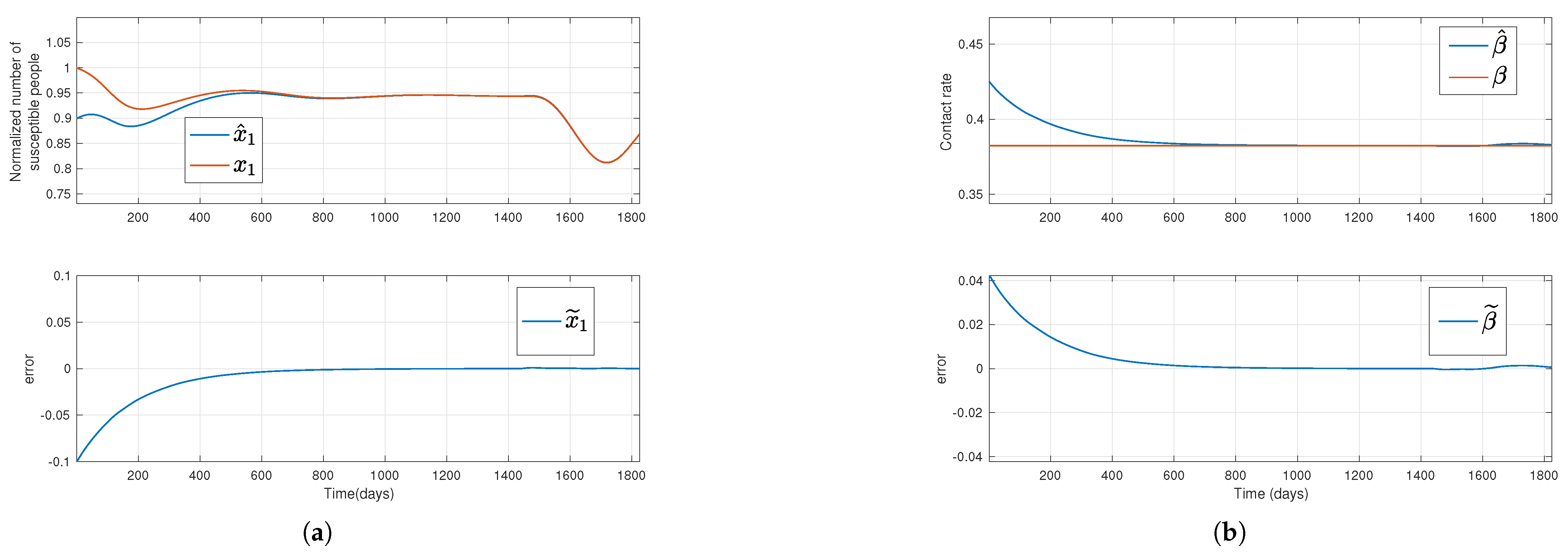
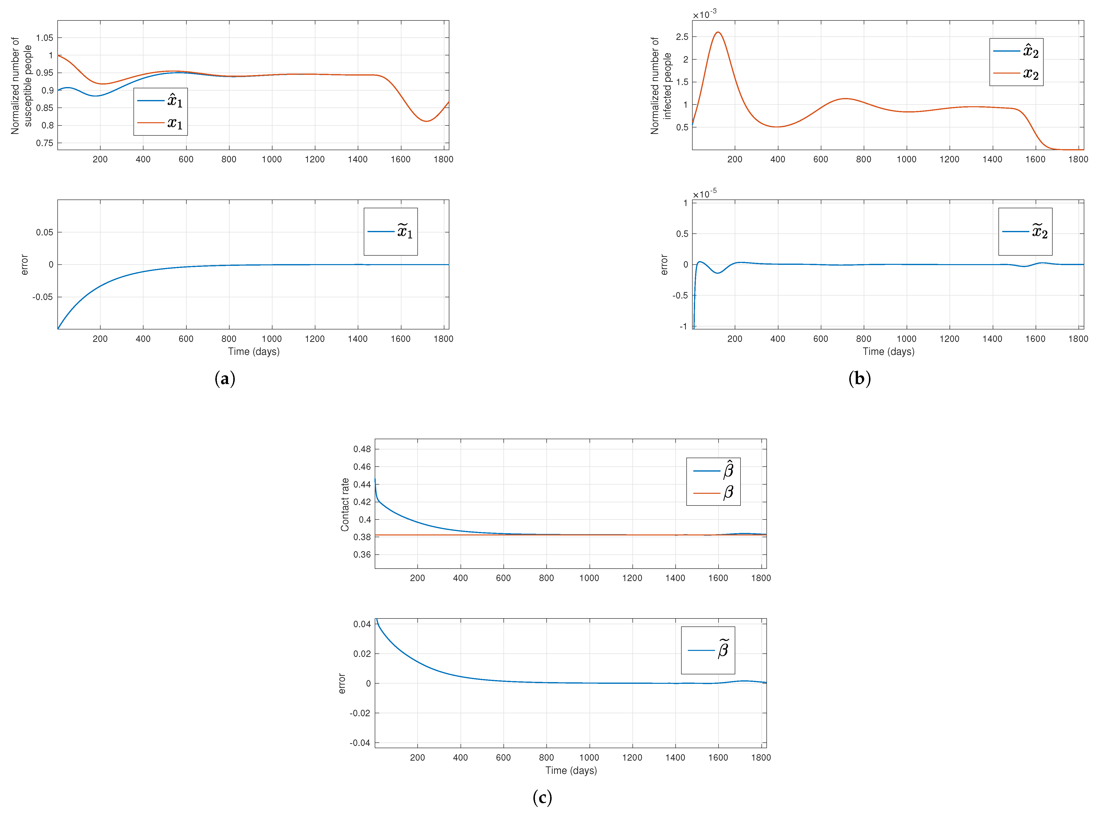
Figure 1.
Solutions of the simulated system (red lines) and their estimation (blue lines) for a constant transmission rate, where the top plots in subfigures (a,b) stand for the susceptible normalized subpopulation and the transmission rate, respectively, considering that the outputs new hospitalizations and new deaths are available. Bottom plots display the error between simulated data and their estimates.
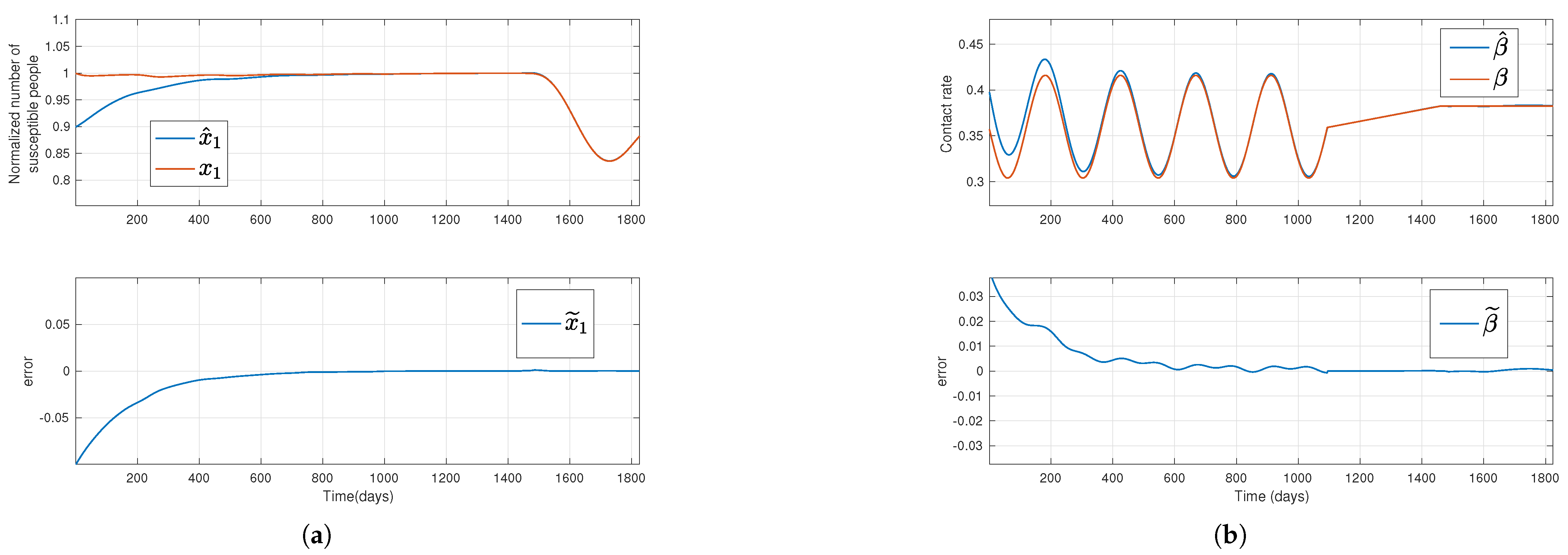
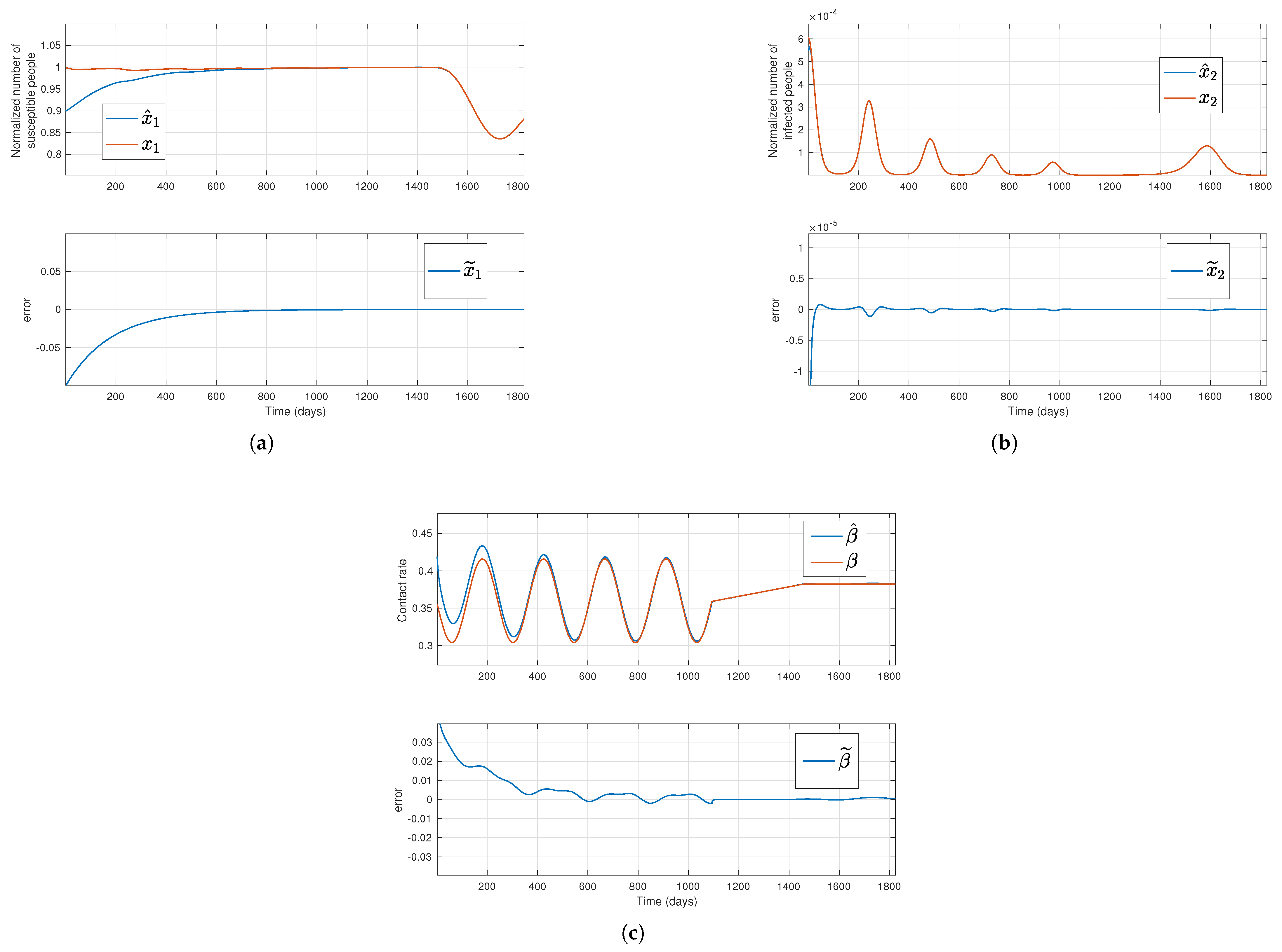
Figure 2.
Solutions of the simulated system (red lines) and their estimation (blue lines) for a time-varying transmission rate, where the top plots in subfigures (a,b), respectively, stand for the susceptible normalized subpopulation and the transmission rate, respectively, considering that the outputs new hospitalizations and new deaths are available. The bottom subfigures display the error between simulated data and their estimates.
6.2. One Output (New Hospitalizations)
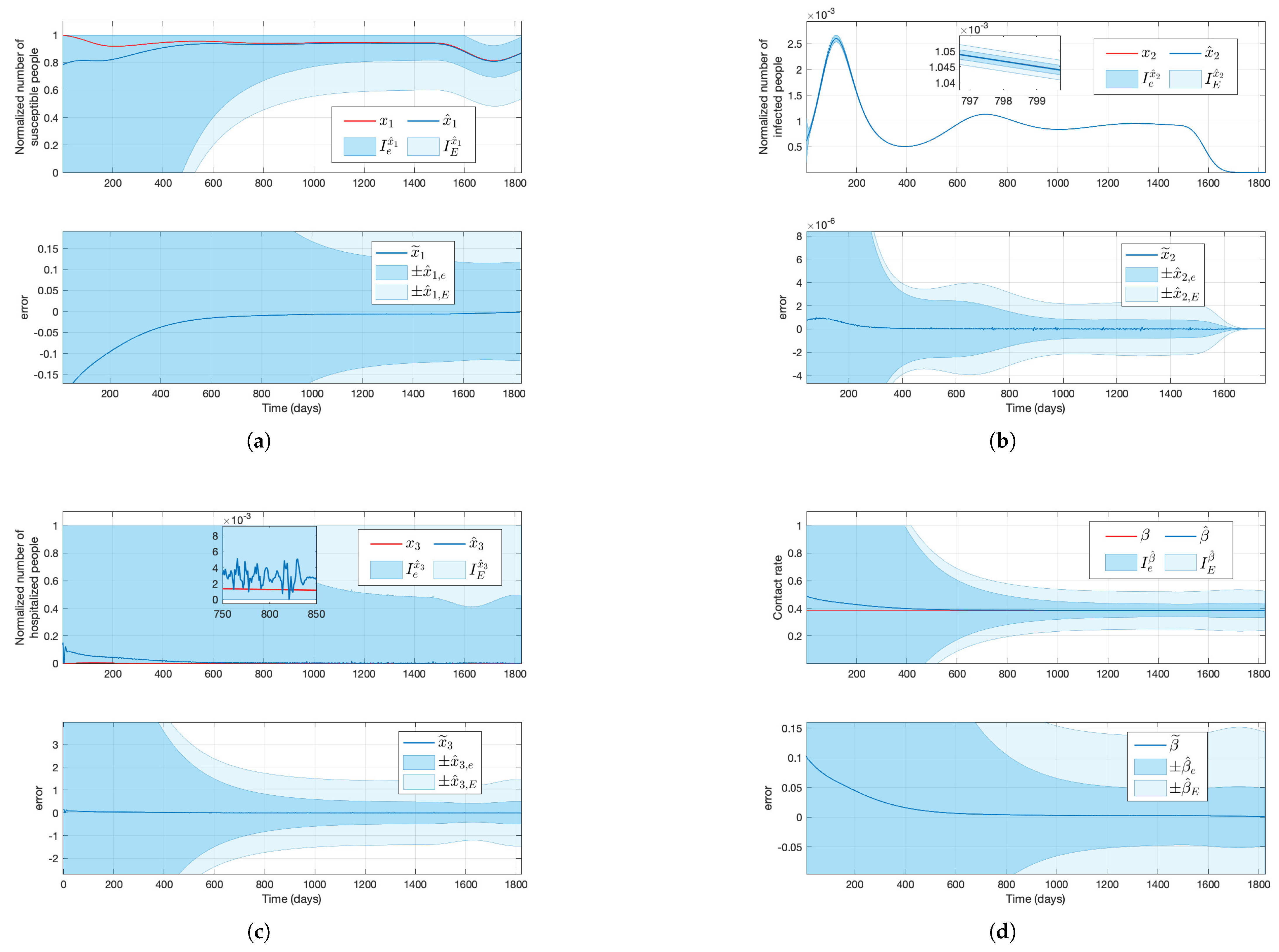
Figure 3.
Solutions of the simulated system (red lines) and their estimation (blue lines), the approximated estimation areas (shaded dark blue areas), and the maximum estimation areas (shaded light areas) for a constant transmission rate, where the top plots in subfigures (a–c) stand for the susceptible, infected, and hospitalized normalized subpopulations, respectively, and the top plot in subfigure (d) stands for the transmission rate, considering that only the output new hospitalizations is available.
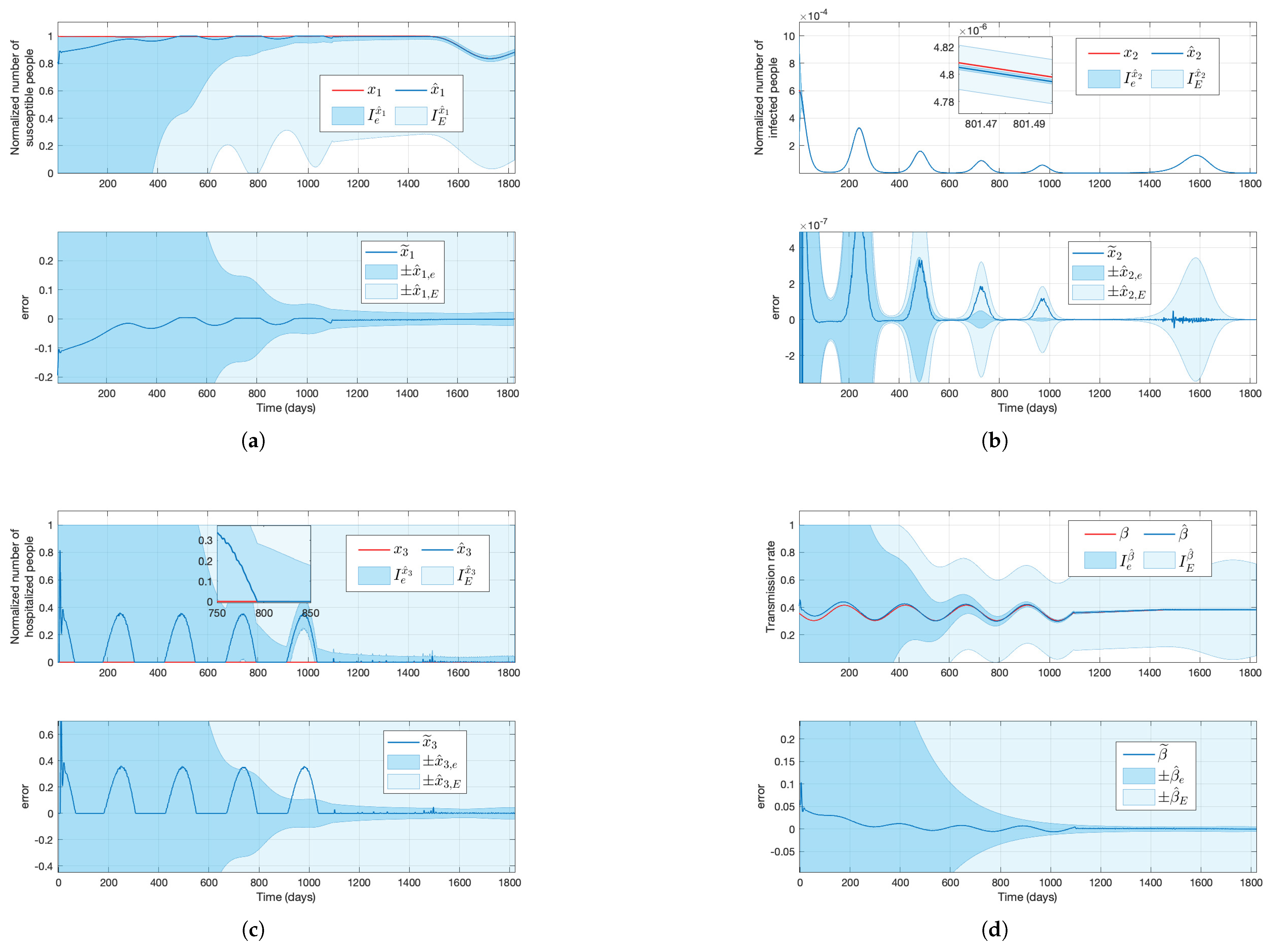
Figure 4.
Solutions of the simulated system (red lines) and their estimation (blue lines), the approximated estimation bound areas (shaded dark blue areas), and the maximum estimation bound areas (shaded light areas) for a time-varying transmission rate, where the top plots in subfigures (a–c) stand for the susceptible, infected, and hospitalized normalized subpopulations, respectively, and the plot in subfigure (d) stands for the transmission rate, considering that only the output new hospitalizations is available.
6.3. One Output (New Deaths)
Regarding the first and third methods, where new admissions in hospitals and new deaths, or only new deaths are assumed to be available, respectively, the estimations for
and
depicted in
Figure 1,
Figure 2,
Figure 5 and
Figure 6 show good results (i.e., after 500 days approximately, the error between the real values and their estimations is quite small) either for constant or time-varying parameter values. However, the estimation response cannot be modified since the observer (
16) convergence is fixed by the term
.
Figure 5.
Solutions of the simulated system (red lines) and their estimation (blue lines), for a constant transmission rate, where the top plots in subfigures (a,b) stand for the susceptible and infected normalized subpopulations, respectively, and the top plot in subfigure (c) stand for the transmission rate, considering that only the output new deaths is available.
Figure 6.
Solutions of the simulated system (red lines) and their estimation (blue lines), where the top plots in subfigures (a,b) stand for the susceptible and infected normalized subpopulations, respectively, and the top plot in subfigure (c) stands for the transmission rate, considering that only the output new deaths is available.
With the estimations
and
, and their respective maximum estimation error, the maximum estimation bounds have been calculated. The real values fall within the range specified by the maximum upper and lower estimation bounds, providing reliable worst-case and best-case scenarios, which are essential in safety and prevention applications (e.g., a controller designed to eradicate a disease considering that there are not any resource limitations). Although
in both simulations, the maximum estimation bounds
are not informative since
and
; see
Figure 3 and
Figure 4.
On the other hand, the approximated estimation errors give tighter bounds, and the values of and also lie within the region and , respectively, for a wide range of t. Even if the time-varying and for provide an approximated region where the real value will lie (i.e., the real values might go outside these regions for some t), it is affordable to consider and instead of and in cases where it is not necessary to consider the worst/best scenario (e.g., if the controller’s purpose is to minimize hospitalizations while saving resources). Overall, and with their respective maximum and approximated estimation bounds give valuable information. In contrast, due to the significant difference between and , in addition to the big values of the maximum and approximated estimation bounds, this method is not appropriate for estimation.
7. Results
This work presents an SIHR epidemic model, whose normalized form is characterized by a set of differential equations with a state vector , and based on the most commonly reported data such as the new hospital admissions per day () or the new deaths per day (), different state and time-varying transmission rate estimation methods have been developed, so any of these will suit users’ needs.
In the first method, both datasets are assumed to be available, and an exponential observer for the state and the transmission rate estimation is proposed. In the second method, only is considered as the system’s output, and the nonlinear dynamical system is transformed into the observer canonical form with the change of variable , which is a diffeomorphism obtained from an output injection and an output diffeomorphism. Once the system is transformed to this new form, an adaptive observer is proposed, so the estimations and are obtained. Finally, the diffeomorphism is applied to obtain . When the change of variables was being built up, two assumptions were made: (i) the terms are negligible for ; (ii) varies slowly with respect to time (). Due to these approximations, the model in its canonical form contains errors, causing the computed estimations to deviate from real values. Without additional information, these deviations remain uncertain. However, assuming that the bounds of those errors are known, equations to calculate the maximum estimation upper () and lower () bounds of , and the maximum estimations of the upper () and lower () bounds of for are obtained, so and for . Given more information about the uncertainties, approximated estimations of the upper () and lower () bounds of , and approximated estimations of the upper () and lower () bounds of for can be obtained; these bounds are closer to the real values than the maximum estimation bounds, but it is not for certain that the real values will lie within the region delimited by those bounds all the time. In the third method, where only the output is considered, an explicit expression to compute is given, which enables the usage of the previously constructed methods.
Although all the proposed methods are validated by a theoretical background, some simulations have been carried out to illustrate the results. With the parameters corresponding to the COVID-19 epidemic, predefined initial state values, a vaccination function, and a transmission rate function, the SIHR epidemic model has been simulated. For each method, the corresponding output has been provided (e.g., to validate the second method, the output has been gathered from simulated data), and the estimations have been computed. Note that, in the third method, after computing from the output , for simplicity reasons, we turn to the first method instead of the second.
The first and the third methods have the advantage of giving good estimations, despite a fixed convergence. With the second method, in addition to obtaining and for , the maximum estimation bounds were also computed along with the error bounds. Then, the conditions and for were evaluated and found to be true. Given the average values of the errors, the approximated estimation error bounds were calculated, and they were shown to be more informative than the maximum estimation bounds since their values were closer to the real ones and the conditions and for were generally satisfied. However, considering the big difference between and the calculated estimation bounds, it follows that this method is not appropriate for .
8. Conclusions
When data on new hospital admissions and new deaths, or only new deaths, are available, the proposed observers and numerical differentiation enable an accurate estimation of both state variables and the transmission rate. However, since numerical differentiation is highly sensitive to noise, smoothing the data is recommended to prevent error amplification. Additionally, these observers require a fixed convergence time to produce reliable estimates, which can be a limitation for short time-series datasets.
When only new hospital admissions data are available, the proposed method does not yield exact estimates but instead provides bounds within which the true values are expected to lie. Determining these bounds requires prior knowledge of certain parameters, such as upper limits for the transmission rate and the number of deaths. While this approach produces reasonably accurate bounds for the susceptible subpopulation and transmission rate, it struggles to define a suitable bound for hospitalized cases. Furthermore, as this method relies on an observer, its estimates are restrained to a convergence time. Compared to previous methods, its numerical implementation is also more complex, requiring the solution of dynamical equations, application of error propagation formulas, and other computational steps.
For large datasets, such as those related to the COVID-19 epidemic, the proposed observer’s convergence is ensured. Consequently, these methods enable the estimation of the transmission rate and provide valuable insights into its dynamics, aiding the development of more effective control policies. For instance, if the estimated transmission rate consistently increases during the winter seasons, strengthening vaccination efforts in the preceding months could help to prevent hospitalizations and deaths during winter.
While controlling disease spread is the primary goal, it cannot be achieved without a validated model. Validating the model and the proposed estimation methods is not as straightforward as simply collecting real data and estimating the time-varying transmission rate and state variables. Commonly, a model is said to be validated if the model can closely reproduce real data. Therefore, a challenge arises: if the susceptible subpopulation and transmission rate are computed using the proposed model and methods, how can these outputs be compared to the real values when no direct data exist for either the susceptible subpopulation or the transmission rate? To address this, future work will focus on transmission rate characterization by establishing a mathematical relationship between the transmission rate and correlated and measurable variables, such as mobility and seasonal changes. This relationship will enable the estimation of the transmission rate from available data, which will then be used to simulate the SIHR epidemic model. Finally, validation will be performed by comparing the model’s predictions (e.g., new hospital admissions and deaths) with real data to assess its accuracy.
A successfully validated model will not only enable accurate disease spread predictions but also provide a framework for designing optimal control strategies.


