Advancing Fault Detection in Distribution Networks with a Real-Time Approach Using Robust RVFLN

Abstract

In this paper, the fault type and location of high-impedance short-circuit faults, which are difficult to detect in distribution networks, are determined in real time using the Real-Time Digital Simulator (RTDS). In this study, an IEEE 39-bar system model is created using the Real-Time Simulation Software Package (RSCAD). In this model, a short-circuit fault is generated at different fault impedance values. For high-impedance short-circuit fault detection, 14 feature vectors are created. Six of these feature vectors are newly developed, and it is found that these six new feature vectors contribute 10% to the detection of hard-to-detect high-impedance short-circuit faults. We propose a data-driven online algorithm for fault type and location detection based on robust regularized random vector function networks (ORR-RVFLNs). Moreover, the robustness of the model is improved by adding a certain amount of noise to the detected short-circuit fault data. In this study, the method ORR-RVFLN for the 39-bus system IEEE detects the average error type for all error impedances, with 92.2% success for the data with noise added. In this study, the fault location is shown to be more than 90% accurate for distances greater than 400 m.

1. Introduction

In distribution networks, it is crucial to ensure the safe and high-quality delivery of electricity to the end user [1,2]. Today, distribution grids have become quite complex [3,4]. The main reasons for this complexity are the inclusion of renewable energy sources, electric vehicles, and electric energy storage systems in distribution grids [5]. Due to this complex network structure, distribution networks are considered highly intensive networks [6,7]. According to previous studies, 80% of the failures occurring in power transmission and distribution systems occur in distribution networks [8,9]. Failures in distribution networks also damage national economies. For example, according to the report provided by the European Network of Transmission System Operators for Electricity (ENTSO-E), in 2020, a total of 1589 faults occurred in the Baltic and Scandinavian countries, resulting in a loss of 2257.2 MWh in the energy supply. Moreover, 55.125% of the faults in the electricity systems of the Baltic and Scandinavian countries are caused by faults in distribution networks [10]. Therefore, fault location and fault type analysis are critical for the safe and stable operation of distribution networks [11,12]. Such interruptions are caused by various types of short-circuit faults in distribution networks. These faults consist of double-phase ground faults (2 ph-g), single-phase ground faults (1 ph-g), and phase phase (2 ph) faults. In distribution networks, 70% of these faults are single-phase ground faults, 15% are two-phase faults, 10% are two-phase ground faults, and 5% are three-phase (3 ph) faults [13,14,15].

These faults occurring in distribution networks are detected by conventional protection devices such as protection relays and overcurrent relays. However, high-impedance faults (HIFs) may not be detected by conventional protection devices due to their low current amplitude [16,17]. In particular, 17.5% of HIFs cannot be detected by conventional protection methods [18]. High-impedance faults (HIFs) represent 5 to 20% of the faults occurring in distribution networks (DNs) [19]. The most prominent characteristic of HIFs is that they are subjected to an electric shock, creating arcing, which poses a great risk to humans and animals. HIFs are identified as the second-largest cause of fatalities related to distribution networks in Brazil. Specifically, in 2013 and 2014, HIFs resulted in 30 and 53 fatalities in Brazil, respectively [12,20]. HIFs are a problem that usually exists in power transmission and distribution systems and also cannot be detected by conventional protection mechanisms. Hence, an intelligent mechanism is required to learn the patterns of different systems belonging to different distribution networks [21,22].

There are many studies in the literature on fault type and location detection using traditional machine learning classification methods [23,24,25]. In Sowah et al., fault detection was performed using a decision tree, but the decision tree method has the disadvantage of overfitting [26]. Rathore et al. performed fault detection using artificial neural networks (ANN), but they had a slow learning rate [27]. Rathore and Shaik performed fault type detection using an ANN algorithm for three-phase current and voltage data obtained from a 400 kV, 2-bus model [28]. Yadav and Swetapadma created a 400 kV, 200 km, two-bus, two-generator, and two-load model. Using three-phase current and voltage magnitude and three-phase current angle data from this model, the fault type and fault location were determined via the fuzzy logic method [29]. Ravesh et al. used support vector machines (SVMs) for fault detection, but the SVM method has the disadvantage of requiring a large amount of memory [30]. Gopakumar et al. created a 400 kV, 300 km, two-bus, two-generator, and two-phasor-measurement-unit (PMU) model in the Matlab/Simulink simulation program. Using the features of the three-phase current and voltage phase angle information obtained from this simulation, fault type detection was performed with SVM [31]. In Shi et al., fault detection was performed using the sparse representation method, but this has the disadvantage of limited processing power for big data [32]. Ghaemi et al. used random forest (RF) for fault detection, but this has the disadvantage of being quite slow [33]. Gangwar et al. used K-Nearest Neighbors for fault detection. However, this method has disadvantages such as being sensitive to noise and outliers [34]. Ananthan et al. built a two-bus, 200 km, and 400 kV transmission line model in the laboratory. Using the LabVIEW program, data from this actual system were extracted and fault type detection was performed with a wavelet transform-based multiresolution analysis (MRA) filter [35]. Salehi and Namdari’s 500 kV, 350 km, two-bus transmission line model was created in the Matlab/Simulink simulation program. The three-phase current data were analyzed using a morphological edge detection (MED) filter to extract distinguishing features, and fault type detection was performed [36]. In Chen et al., fault detection was performed using the extreme learning machine (ELM). However, this method has the disadvantage of not being able to train large data quickly and efficiently [15]. Tong et al. performed fault detection using convolutional neural networks (CNN). However, training CNNs takes a long time, especially with large data sets [37]. In Taheri et al., the long short-term memory (LSTM) algorithm was proposed to detect fault types and locations. However, this method also has the disadvantage that it is prone to overfitting [38]. Hu et al. performed fault detection using deep graph learning methods. However, this type of method is not robust to noise in the data [39]. In Ding et al., the MCECA-CloFormer method was proposed as a novel approach for single-phase ground fault detection in distribution networks. The method utilizes zero-sequence current signals as the primary input data, representing a significant advancement in the field [40]. Sodin et al. proposed a method for fault detection that supports phasor measurement unit (PMU)-based fault detection and localization [41]. Wan et al. developed a dynamic Bayesian network (DBN)-based model for the normal operation of cables and the detection of different types of faults. In this study, the fault location is also determined with high accuracy [42]. Shoudong Xu et al. endeavored to detect a single-phase short circuit fault in a distribution network with distributed generators. The magnitude and phase angle differences of the current vectors were utilized to locate the single-phase fault [43].

In the literature, although short-circuit faults are very common, there are few studies that investigate the detection of high-impedance faults and sensor-induced noise. In this paper, we describe a new algorithm to detect the fault type and location in distribution networks using random vector functional link networks (RVFLN). The proposed algorithm uses three-phase current and three-phase voltage measurements to generate a feature vector for the fault type and location. Of these 14 feature vectors, six of them are newly developed for the detection of high-impedance faults. In this way, a 10% success increase is achieved in the detection of high-impedance faults. In this study, we first build a single-bus transmission system in the PSCAD simulation program and use the simulation data to train the model for fault type and location detection. In this single-bus transmission system, the fault type and location are detected with high accuracy. We then analyze the performance of the model in multi-bus systems that we encounter in real-life distribution networks. For this purpose, the IEEE 39-bus system is modeled using the Real-Time Digital Simulator (RTDS) for fault type and location detection. Data are taken from faults of different types and impedances generated in the model. Then, a certain amount of noise is added to these data to test the robustness. The results obtained from the proposed algorithm are compared with those of the convolutional neural network (CNN), long short-term memory (LSTM), support vector machine, and extreme learning machine (ELM) classification algorithms. The main contributions of this study can be explained as follows.

1

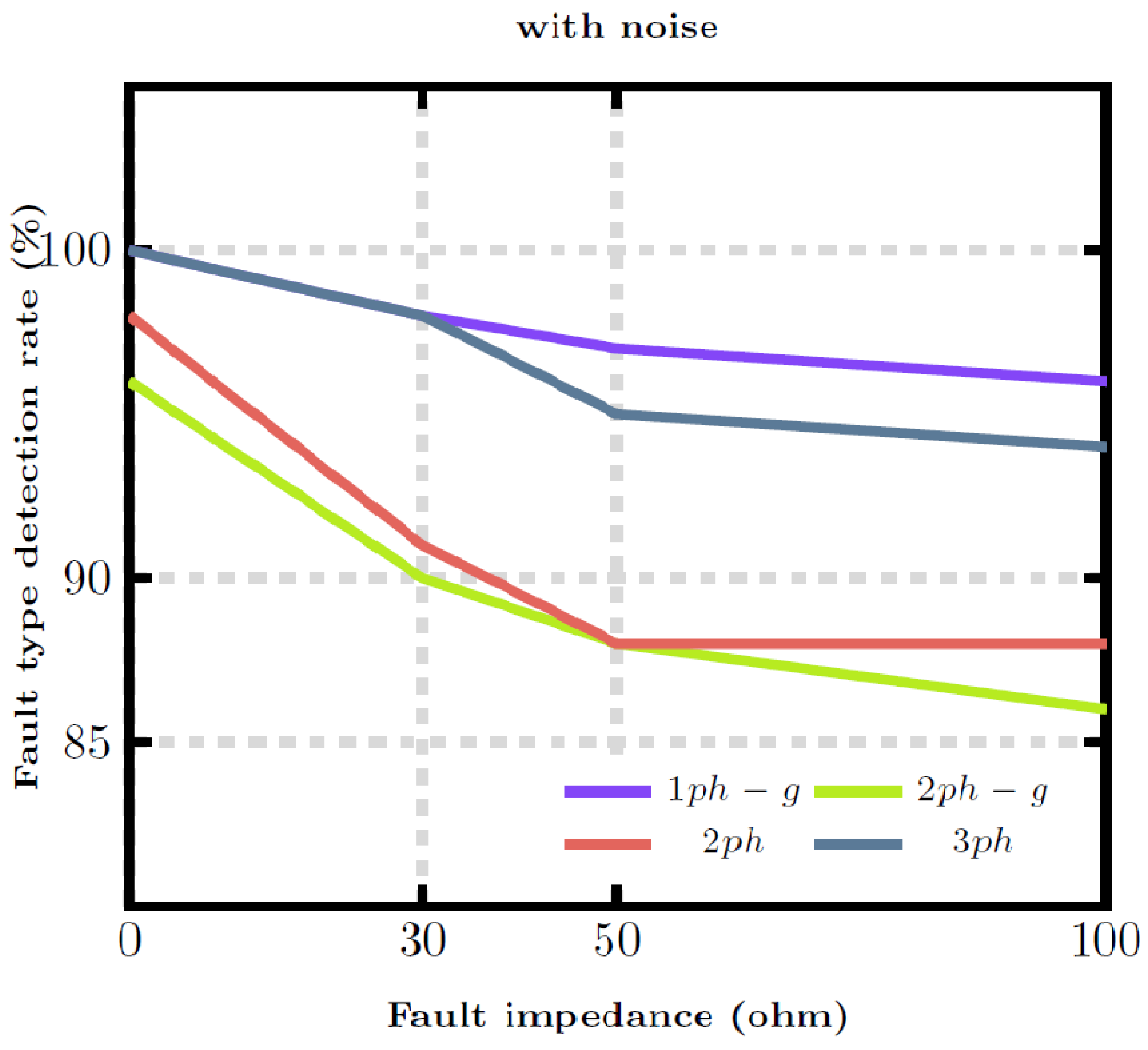
When noise from sensors is not taken into account in real-time operations, various problems occur in both signal processing and machine learning applications. The main problems are misclassification and low accuracy. However, in this study, noise and outlier effects are taken into account for fault detection.

2

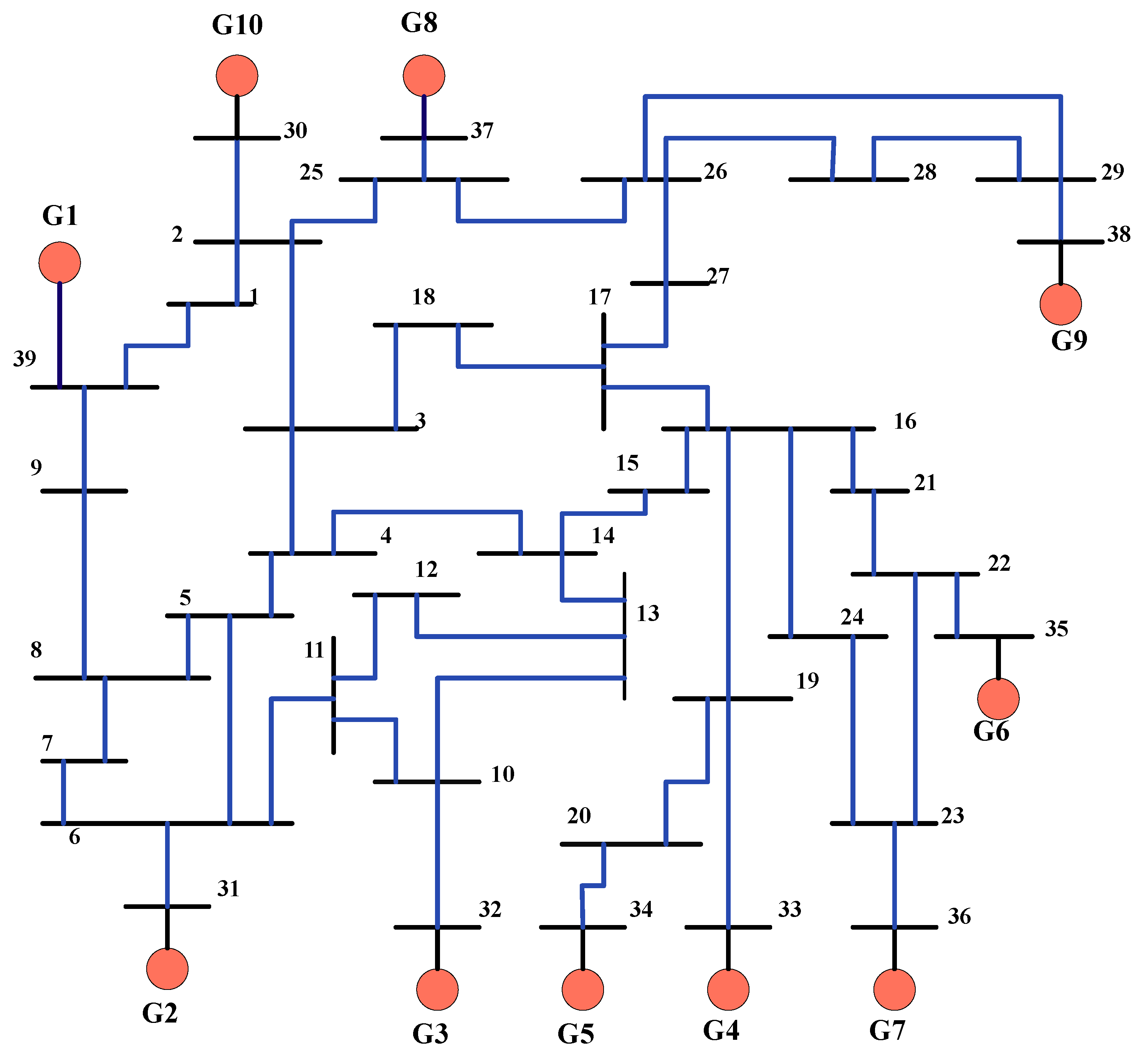
When the studies in the research are examined, Matlab is generally used for the realization of fault type and location detection in single-bus transmission systems. However, the work done in Matlab needs to be compared with real-time systems. In this study, the IEEE 39-bus system, which is a small model of a distribution network, is realized using the RTDS simulator and a real-time study is performed.

3

When refs. [18,19,20,21,22,23,24,25,26,27,28,29,30,31,32,33,34,35,36,37,38,39,40] are analyzed, it is found that six new attribute vectors that were not previously used in fault type data detection in distribution networks have been created. Thanks to these feature vectors, the accuracy of fault type and location detection in high-impedance short-circuit faults is improved by 10%.

4

In the literature [16,17,18,19,20,21,22,23,24], high-impedance short-circuit faults are evaluated together with other faults and an average detection accuracy rate is given. In general, the detection of high-impedance faults is not considered separately in previous research.

The paper is organized as follows. Section 2 presents the ORR-RVFLN algorithm, feature vector extraction, and formulation; Section 3 presents the IEEE 39-bus system in the RTDS and the single-bus transmission system in PSCAD; and Section 4 presents the fault type and location detection values. Finally, the paper concludes in Section 5.

2. Fault Detection Method

2.1. Feature Construction

In order to determine the types and locations of faults occurring in a distribution network and to distinguish them from normal system operation, fault data should be prepared. In our study, firstly, 3-phase current and 3-phase voltage data were taken in the single-bus transmission system created in the PSCAD simulation program. From these data, attribute vectors were created, as given in

Table 1. Feature vectors for fault detection.

Feature	Notation	Formulation
U1	$In\left(t\right)$	current magnitude
U2	$Vn\left(t\right)$	voltage magnitude
U3	$\phi In\left(t\right)$	current angle
U4	$\phi Vn\left(t\right)$	voltage angle
U5	$d/dt\left(In\right(t\left)\right)$	derivative of current magnitude
U6	$d/dt\left(Vn\right(t\left)\right)$	derivative of voltage magnitude
U7	$d/dt\left(\phi In\right(t\left)\right)$	derivative of current angle
U8	$d/dt\left(\phi Vn\right(t\left)\right)$	derivative of voltage angle
U9	${∥\begin{array}{c}{\mathbf{V}}_n\end{array}∥}_1$	${\displaystyle \sum _{j=1}^{360}\left|\begin{array}{c}{\mathbf{S}}^j\end{array}\right|}$
U10	${∥\begin{array}{c}{\mathbf{V}}_n\end{array}∥}_2$	${\left[\begin{array}{c}{\displaystyle \sum _{j=1}^{360}(S^j{)}^2}\end{array}\right]}^{1/2}$
U11	${∥\begin{array}{c}{\mathbf{V}}_n\end{array}∥}_{\infty }$	$\underset{j}{max\left|\begin{array}{c}{\mathbf{S}}^j\end{array}\right|}$
U12	${∥\begin{array}{c}{\mathbf{I}}_n\end{array}∥}_1$	${\displaystyle \sum _{j=1}^{360}\left|\begin{array}{c}{\mathbf{S}}^j\end{array}\right|}$
U13	${∥\begin{array}{c}{\mathbf{I}}_n\end{array}∥}_2$	${\left[\begin{array}{c}{\displaystyle \sum _{j=1}^{360}(S^j{)}^2}\end{array}\right]}^{1/2}$
U14	${∥\begin{array}{c}{\mathbf{I}}_n\end{array}∥}_{\infty }$	$\underset{j}{max\left|\begin{array}{c}{\mathbf{S}}^j\end{array}\right|}$

. These 14 attribute vectors were created by considering different fault types and fault impedance values. Feature vectors U1, U2, U3, and U4 represent the magnitudes of the current and voltage ($\phi In\left(t\right)$, $\phi Vn\left(t\right)$) and their angles ($\phi In\left(t\right)$, $\phi Vn\left(t\right)$) to prevent parameter readjustment in the distribution network. U5 and U7 denote instantaneous changes in the current and its angle. U6 and U8 refer to instantaneous changes in the voltage and its angle. Finally, the remaining 6 feature vectors can be transformed from raw data into discriminative features through signal norms [44]. U9, U10, and U11 are the 1, 2, and infinity norms from the raw voltage data, respectively (${\ell }_1,{\ell }_2\mathrm{and}{\ell }_{\infty }-norms$), which are used to obtain the appropriate signal characteristics. From the raw current data U12, U13, and U14, appropriate signal characteristics are obtained with norms 1, 2, and infinity.

The feature vectors in Table 1 are carefully selected to capture both the time-domain and frequency-domain characteristics of the electrical signals in the distribution network. These features are designed to enhance the fault classification and localization performance, especially for HIFs, which exhibit subtle signal variations.

2.1.1. Fundamental Electrical Features (U1–U4)

These feature vectors represent fundamental electrical parameters extracted from voltage and current waveforms.

• U1—Represents the absolute magnitude of the current waveform in each phase. Changes in this value can indicate the presence of a fault.
• U2—Represents the absolute magnitude of the voltage waveform in each phase. A significant drop in voltage is often a sign of a fault.
• U3—The phase angle of the current relative to a reference point, providing insights into power flow and fault-induced distortions.
• U4—The phase angle of the voltage, which can shift significantly during a fault event, particularly in unbalanced conditions.

These fundamental features are critical in distinguishing between normal and faulty operating conditions in the distribution network.

2.1.2. Derivative-Based Features (U5–U8)

These feature vectors are designed to capture dynamic changes in voltage and current signals, which are especially useful in detecting transient disturbances caused by faults.

• U5—Measures the rate of change in the current, highlighting rapid variations indicative of fault inception.
• U6—Captures sudden voltage drops or fluctuations caused by fault conditions.
• U7—Provides insights into frequency variations and phase shifts due to faults.
• U8—Tracks dynamic phase shifts in voltage waveforms, particularly useful in detecting unbalanced faults.

These features improve the fault classification accuracy, as traditional magnitude-based methods often fail to distinguish between different types of faults, particularly HIFs, which cause minimal changes in magnitude but affect the waveform dynamics.

2.1.3. Norm-Based Statistical Features (U9–U14)

To further enhance the fault detection accuracy, we introduce norm-based transformations of the raw current and voltage signals. These features are essential in capturing subtle waveform variations and ensuring robustness to noise.

• U9—Represents the sum of the absolute values of voltage samples over a defined window, effectively capturing the total signal intensity.
• U10—Reflects the root mean square (RMS) value of the voltage signal, emphasizing the dominant frequency components.
• U11—Extracts the maximum absolute value in the voltage signal, highlighting peak disturbances.
• U12—Represents the sum of the absolute values of current samples, useful in quantifying the total current deviation.
• U13—Provides an RMS-like measurement for the current, emphasizing significant fluctuations.
• U114—Extracts the maximum absolute value in the current signal, useful in detecting extreme deviations due to faults.

These statistical features enhance the robustness against noise and small signal variations, particularly in scenarios where traditional amplitude-based features fail to provide clear fault indicators.

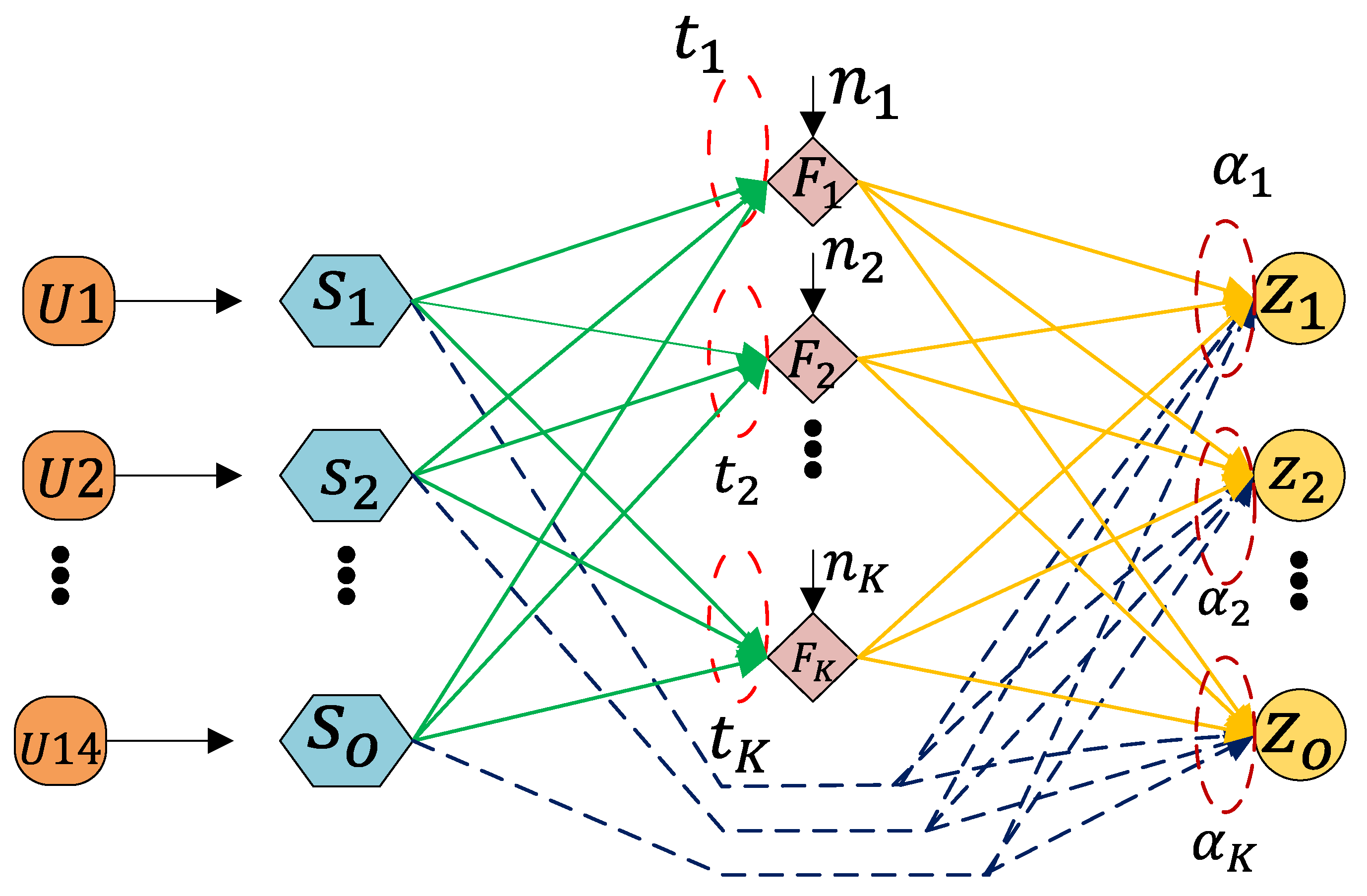
2.2. RVFLN Algorithm

The RVFLN algorithm was published in 1992 by Pao et al. as a single-hidden-layer feed-forward network [45]. Figure 1 shows the basic structure of RVFLN. Since its development, the RVFLN model has been successfully used for regression and classification in various engineering applications [46,47,48]. However, it has not been used for fault type and location detection in distribution networks. The main advantage of this method is that the weights between the input layer and the hidden layer are randomly assigned [49,50]. It also has the advantage of calculating the output weights using the least squares (LS) algorithm. Another advantage of this method is that it can process data in real time for engineering applications [51,52].

The data consist of training samples, $D=\left\{(s_o,z_o)|o=1,\dots ,N\right\}\subset {\mathbf{R}}^d\times R$. This is indicated as a special type of SLFN with K hidden nodes [53].

$${\displaystyle h\left(s\right)=\sum _{u=1}^K{\alpha }_u{f}_u(t_u,n_u,s)}$$

(1)

$t_u$ and $n_u$ are hidden node parameters. Between the hidden layer node and the output node is ${\alpha }_u$, which is also defined as the output weight. $f_u$ can be used as a radial basis activation function.

$$f_u=f\left({\displaystyle \frac{∥\begin{array}{c}s-t_u\end{array}∥}{n_u}}\right)t_u\in {\mathbf{R}}^d,n_u\in R^{+}$$

(2)

The norm ${\ell }_2$ is indicated by $\parallel •\parallel$. The sum of squared errors is preferred as a cost function for N samples $(s_o,z_o)\subset {\mathbf{R}}^d\times R$.

$${\displaystyle V=\sum _{o=1}^N{∥\begin{array}{c}{\displaystyle \sum _{u=1}^K{\alpha }_u{f}_u(t_u,n_u,s_o)-z_o}\end{array}∥}^2}$$

(3)

In the RVFLN algorithm, the hidden node parameters ($t_u$ and $n_u$) can be given randomly. However, the linear parameters of the output layer are calculated analytically. Using Equation (3), a quadratic optimization problem is obtained.

$$\underset{\alpha }{argmin}{∥\begin{array}{c}\mathbf{F}\alpha -\mathbf{Z}\end{array}∥}^2,$$

(4)

$$F={\left[\begin{array}{ccc}f(t_1,n_1,s_1)& \cdots & f(t_K,n_K,s_1)\\ ⋮& \ddots & ⋮\\ f(t_1,n_1,s_N)& \cdots & f(t_K,n_K,s_N)\end{array}\right]}_{N\times K}$$

(5)

$$\alpha ={\left[\begin{array}{c}{\alpha }_1\\ ⋮\\ {\alpha }_K\end{array}\right]}_{K\times 1}and\mathbf{Z}={\left[\begin{array}{c}{z}_1\\ ⋮\\ z_N\end{array}\right]}_{N\times 1}$$

(6)

$\mathbf{F}$ is the hidden layer output. $\mathbf{Z}$ is the sampled output. $\alpha$ is the sampled output’s weight. The optimal output weight $\alpha$ is calculated as in Equation (7).

$$\alpha ={\mathbf{F}}^{†}\mathbf{Z}$$

(7)

${\mathbf{F}}^{†}$ can be described as the Moore–Penrose generalized inverse of $\mathbf{F}$. According to the results described in [53,54], fixed coverage for t and n does not guarantee the modeling performance. Therefore, when using RVFLN, it is necessary to pay sufficient attention to this scope setting. One way to solve this scope setting problem is to assign arbitrary parameters from the $[\lambda ,+\lambda ]$ variable’s scope. It is also necessary to choose a reasonable value according to some specific criteria.

2.3. R-RVFLN

The regularized RVFLN (R-RVFLN) effectively avoids the overfitting problem of the model and reduces the magnitude of the output weight. This also reduces the model complexity. Using the method in [53,55], a regular term $\left({\ell }_{2}norm\right)$ is added to the objective function. With this added term, an R-RVFLN algorithm is generated by ridge regression. For a given N distinct samples $(s_o,z_o)$, the R-RVFLN with norm ${\ell }_2$ is as given in Equation (8).

$${\displaystyle min:V=\frac{1}{2}{∥\begin{array}{c}\alpha \end{array}∥}_2^2+\frac{B}{2}\sum _{o=1}^N{\epsilon }_o^2,s.t:\mathbf{f}\left({\mathbf{s}}_{\mathbf{o}}\right)\alpha =z_o-{\epsilon }_o,\forall o}$$

(8)

B is the regularization parameter. The task of this parameter is to balance the training error and the output weight norm; ${\sum }_{o=1}^N{\epsilon }_o^2$ and ${∥\begin{array}{c}\alpha \end{array}∥}_2^2$ denote empirical and structural losses, respectively. According to the regularized LS algorithm, the solution of $\alpha$ is as given in Equation (9).

$$\alpha =\left\{\begin{array}{cc}{({\mathbf{F}}^T\mathbf{F}+{\displaystyle \frac{1}{B}})}^{-1}{\mathbf{F}}^T\mathbf{Z}\hfill & ,N\ge K\hfill \\ {\mathbf{F}}^T{(\mathbf{F}{\mathbf{F}}^T+{\displaystyle \frac{1}{B}})}^{-1}\mathbf{Z}\hfill & ,N<K\hfill \end{array}\right.$$

(9)

Equation (9) is described as the offline learning form of the R-RVFLN. As described in [53,56], the online learning form describes a recursive solution.

$$\left\{\begin{array}{c}{\mathbf{V}}_m={\mathbf{V}}_{m+1}+{\mathbf{F}}_m^T{\mathbf{F}}_m\hfill \\ {\alpha }_m={\alpha }_{m-1}+{\mathbf{V}}_m^{-1}{\mathbf{F}}_m^T({\mathbf{Z}}_m-{\mathbf{F}}_m^T{\alpha }_{m-1})\hfill \end{array}\right.$$

(10)

${\mathbf{F}}_m$ is called the hidden layer output for the m-th instance. The initial values of the model are expressed as in Equation (11).

$$\left\{\begin{array}{c}{\mathbf{V}}_0={\mathbf{F}}_0^T{\mathbf{F}}_0+{\displaystyle \frac{\mathbf{1}}{\mathbf{B}}}\hfill \\ {\alpha }_0={\mathbf{V}}_0^{-1}{\mathbf{F}}_0^T{\mathbf{Z}}_0\hfill \end{array}\right.$$

(11)

One advantage is that the online R-RVFLN model can be initialized using a small number of samples. Another advantage is that the output weight norm is relatively small. It also has disadvantages. The greatest disadvantage is that, when there are data with outliers, the quality of the online R-RVFLN may deteriorate. In this case, the regularization parameter B may not run correctly, leading to algorithm misfitting.

2.4. RR-RVFLN

In [57], a weighted empirical lossy ridge-type regularized RVFLN algorithm is derived using the nonparametric kernel density estimation (NKDE) method. This new method solves the robustness problem and is called the robust regularized RVFLN (RR-RVFLN). It is explained that, in RR-RVFLN, empirical loss weights are calculated according to the reliability of the samples estimated by the NKDE method. Reducing the effect of outliers through this method depends on decreasing and increasing the empirical loss weights of low- and high-reliability samples. The RR-RVFLN formula for N different samples $(s_o,z_o)$ is expressed as in Equation (12).

$$\begin{array}{cc}\hfill & {\displaystyle min:\frac{1}{2}{∥\begin{array}{c}\alpha \end{array}∥}_2^2+\frac{B}{2}\sum _{o=1}^N{r}_o{∥\begin{array}{c}{\epsilon }_o\end{array}∥}_2^2}\hfill \\ \hfill & s.t:\mathbf{f}\left({\mathbf{s}}_{\mathbf{o}}\right)\alpha =z_o-{\epsilon }_o,\forall o.\hfill \end{array}$$

(12)

$r_o$ is defined as the empirical loss weight of the sample.

According to the information given in the Karush–Kuhn–Tucker (KKT) theorem, we have the optimization problem given in Equation (12). This problem is equivalent to the binary optimization problem in Equation (13).

$$\begin{array}{cc}\hfill {\mathbf{V}}_{{\ell }_2}(\alpha ,\epsilon ,\beta )& {\displaystyle =\frac{1}{2}{∥\begin{array}{c}\alpha \end{array}∥}_2^2+\frac{1}{2}B\sum _{o=1}^N{r}_o{\epsilon }_o^2}\hfill \\ \hfill & {\displaystyle -\sum _{o=1}^N{\beta }_o(\mathbf{f}\left({\mathbf{s}}_{\mathbf{o}}\right)\alpha -z_o+{\epsilon }_o)}\hfill \end{array}$$

(13)

${\beta }_o$ is expressed as the Lagrange multiplier corresponding to the o-th input sample. However, in this case, it must satisfy the partial derivative of zero with respect to $\alpha$, $\epsilon$, and $\beta$. In this case, there is only one optimal solution for the resulting convex quadratic optimization problem (see details in [53]).

The empirical loss weights $r_o,o=1,\dots ,N$ are important parameters in solving $\alpha$, while the regularity parameter B can be chosen via the L-curve [58]. $r_o$ describes the contribution of the samples to the solution to increase the robustness of the algorithm and is calculated analytically. In this solution, the contribution of low-density outliers to the solution is small. An identity matrix $\mathbf{R}$ must be constructed to generate the probability distribution of the residuals in RR-RVFLN.

$${\displaystyle {\epsilon }_u=\sum _{o=1}^K{\alpha }_{o}fo({\mathbf{t}}_o,n_o,{\mathbf{s}}_u)-z_u,u=1,2,\cdots ,N}$$

(14)

The probability density function of the residuals can be calculated using Equation (15).

$${\displaystyle h\left(x\right)=\frac{1}{fN}\sum _{u=1}^N\psi \left(\frac{s-{\epsilon }_u}{f}\right)}$$

(15)

$f=1.06\widehat{\zeta }{N}^{{\displaystyle \frac{-1}{5}}}$ s is called the width of the predicted window. $\widehat{\zeta }$ is expressed as the standard deviation of the residuals. $\psi$ is calculated using Equation (16) as a Gaussian kernel function.

$$\psi \left(s\right)={\displaystyle \frac{1}{\sqrt{2\pi }}}{e}^{{\displaystyle \frac{-1}{2}}{s}^2}$$

(16)

Using Equation (15), the probability ${\epsilon }_u$ of each residue is calculated as $h\left({\epsilon }_u\right)$. The reliability of the sample is proportional to the value of $h\left({\epsilon }_u\right)$. The weight of $r_o$ is directly calculated analytically with respect to $h\left({\epsilon }_u\right)$.

2.5. ORR-RVFLN

Parameters such as the correct use of time and cost reduction are important in real life. Therefore, it is necessary to quickly correct the errors that occur in such systems. RR-RVFLN is beneficial in reducing the estimation error but has the disadvantage of time consumption. Therefore, the online robust regulated RVFLN (ORR-RVFLN) has been developed.

2.5.1. $N<K$

A small number of data were generated to construct the first model using Equation (16). Then, ${\mathbf{F}}_{\mathbf{0}}$ and ${\alpha }_0$ were set as first hidden layer output and output weight, respectively. When the kth sample arrives, ${\mathbf{R}}_{\mathbf{0}}$ is initialized as the unit matrix.

$$\alpha ={\mathbf{F}}_m^T{\left({\displaystyle \frac{1}{B}}+{\mathbf{R}}_m{\mathbf{F}}_m{\mathbf{F}}_m^T\right)}^{-1}{\mathbf{R}}_m{\mathbf{Z}}_m,$$

(17)

$${\mathbf{F}}_m=\left[\begin{array}{c}{\mathbf{F}}_{m-1}\\ \rho {\mathbf{F}}_m\end{array}\right]and{\mathbf{R}}_m=\left(\begin{array}{cc}{\mathbf{R}}_m& 0\\ 0& \rho {\mathbf{R}}_m\end{array}\right)$$

(18)

$\rho {\mathbf{F}}_m$ is the hidden layer output. Moreover, $\rho {\mathbf{R}}_m$ is the empirical loss weight.

$$\begin{array}{cc}\hfill {\mathbf{M}}_m^{-1}& ={\left({\displaystyle \frac{1}{B}}+{\mathbf{R}}_m{\mathbf{H}}_m{\mathbf{F}}_m^T\right)}^{-1}\hfill \\ \hfill & ={\left(\begin{array}{cc}{\mathbf{R}}_{m-1}{\mathbf{F}}_{m-1}{\mathbf{F}}_{m-1}^T+{\displaystyle \frac{1}{B}}& {\mathbf{R}}_{m-1}{\mathbf{F}}_{m-1}\rho {\mathbf{F}}_m^T\\ \rho {\mathbf{R}}_m\rho {\mathbf{F}}_m{\mathbf{F}}_{m-1}^T& \rho {\mathbf{R}}_m\rho {\mathbf{F}}_m\rho {\mathbf{F}}_m^T+{\displaystyle \frac{1}{B}}\end{array}\right)}^{-1}\hfill \end{array}$$

(19)

Thanks to the tuning parameter B, $M_m$ can always be calculated by inversion.

$${\mathbf{M}}_m^{-1}=\left(\begin{array}{cc}E& F\\ G& L\end{array}\right)$$

(20)

Equation (21) is obtained by using Equations (19) and (20).

$$\left\{\begin{array}{c}E={\mathbf{M}}_{m-1}^{-1}+{\mathbf{M}}_{m-1}^{-1}{\mathbf{R}}_{m-1}{\mathbf{F}}_{m-1}\rho {\mathbf{F}}_m^T{\mathbf{D}}_m^{-1}\rho {\mathbf{R}}_m\rho {\mathbf{F}}_m{\mathbf{F}}_{m-1}^T{\mathbf{M}}_{m-1}^{-1}\hfill \\ F=-{\mathbf{M}}_{m-1}^{-1}{\mathbf{R}}_{m-1}{\mathbf{F}}_{m-1}\rho {\mathbf{F}}_m^T{\mathbf{D}}_m^{-1},\hfill \\ G=-{\mathbf{D}}_m^{-1}\rho {\mathbf{R}}_m\rho {\mathbf{F}}_m{\mathbf{F}}_{m-1}^T{\mathbf{M}}_{m-1}^{-1}\hfill \\ L=-{\mathbf{D}}_m^{-1}\hfill \end{array}\right.$$

(21)

$$\begin{array}{cc}\hfill {\mathbf{D}}_m& =\rho {\mathbf{R}}_m\rho {\mathbf{F}}_m\rho {\mathbf{F}}_m^T+{\displaystyle \frac{1}{B}}\hfill \\ \hfill & -\rho {\mathbf{R}}_m\rho {\mathbf{F}}_m{\mathbf{F}}_{m-1}^T{\mathbf{M}}_{m-1}^{-1}{\mathbf{R}}_{m-1}{\mathbf{F}}_{m-1}\rho {\mathbf{F}}_m^T\hfill \end{array}$$

(22)

Equation (23) is obtained by using Equations (17) and (22).

$$\alpha ={\mathbf{F}}_m^T{\mathbf{M}}_m^{-1}{\mathbf{R}}_m{\mathbf{Z}}_m$$

(23)

${\mathbf{Z}}_m=[{\mathbf{Z}}_{m-1},\rho {\mathbf{Z}}_m]$. When $N<K$, between Equations (18) and (23), the update algorithm works when mth data arrive. Since ${\mathbf{F}}_m$ contains consecutive examples, a problem arises in which the learning time increases with the accumulation of samples.

2.5.2. $N>K$

Using Equation (16), the mth sample Equation (24) is calculated.

$${\alpha }_m=\left({\mathbf{F}}_m^T{\mathbf{R}}_m{\mathbf{F}}_m+{\displaystyle \frac{1}{B}}\right){\mathbf{F}}_m^T{\mathbf{R}}_m{\mathbf{Z}}_m$$

(24)

where ${\mathbf{M}}_m^{-1}={\left({\mathbf{F}}_m^T{\mathbf{R}}_m{\mathbf{F}}_m+{\displaystyle \frac{1}{B}}\right)}^{-1}$. Using the new $R_m$ and $F_m$ Equation (18), Equation (25) is calculated.

$$\begin{array}{cc}\hfill {\mathbf{M}}_m^{-1}& ={\left({\mathbf{F}}_m^T{\mathbf{R}}_m{\mathbf{F}}_m+{\displaystyle \frac{1}{B}}\right)}^{-1}\hfill \\ \hfill & ={\left(\left[\begin{array}{cc}{\mathbf{F}}_{m-1}^T& \rho {\mathbf{F}}_m^T\end{array}\right]\left(\begin{array}{cc}{\mathbf{R}}_{m-1}& 0\\ 0& \rho {\mathbf{R}}_m\end{array}\right)\left[\begin{array}{c}{\mathbf{F}}_{m-1}\\ \rho {\mathbf{F}}_m\end{array}\right]+{\displaystyle \frac{1}{B}}\right)}^{-1}\hfill \\ \hfill & ={\left({\mathbf{F}}_{m-1}^T{\mathbf{R}}_{m-1}{\mathbf{F}}_{m-1}+\rho {\mathbf{F}}_m^T\rho {\mathbf{R}}_m\rho {\mathbf{F}}_m+{\displaystyle \frac{1}{B}}\right)}^{-1}\hfill \\ \hfill & ={\left({\mathbf{M}}_{m-1}+\rho {\mathbf{F}}_m^T\rho {\mathbf{R}}_m\rho {\mathbf{F}}_m\right)}^{-1}\hfill \end{array}$$

(25)

The Sherman–Morrison–Woodbury formula is given in Equation (26).

$${(E+FGL)}^{-1}=E^{-1}-E^{-1}F{(G^{-1}+L{E}^{-1}F)}^{-1}L{E}^{-1}$$

(26)

The ${\mathbf{M}}_m^{-1}$ can be expressed by

$${\mathbf{M}}_m^{-1}=(\mathbf{I}-{\mathbf{W}}_m\rho {\mathbf{F}}_m){\mathbf{M}}_{m-1}^{-1},$$

(27)

$${\mathbf{W}}_m^{-1}={\mathbf{M}}_{m-1}^{-1}\rho {\mathbf{F}}_m^T{(\rho {\mathbf{R}}_m^{-1}+\rho {\mathbf{F}}_m{\mathbf{M}}_{m-1}^{-1}\rho {\mathbf{F}}_m^T)}^{-1}$$

(28)

Next,

$$\begin{array}{c}\hfill {\left[\begin{array}{c}{\mathbf{F}}_{m-1}\\ \rho {\mathbf{F}}_m\end{array}\right]}^T\left(\begin{array}{cc}{\mathbf{R}}_{m-1}& 0\\ 0& \rho {\mathbf{R}}_m\end{array}\right)\left[\begin{array}{c}{\mathbf{Z}}_{m-1}\\ \delta {\mathbf{Z}}_m\end{array}\right]\\ \hfill ={\mathbf{F}}_{m-1}^T{\mathbf{R}}_{m-1}{\mathbf{Z}}_{m-1}+\rho {\mathbf{F}}_m^T\rho {\mathbf{R}}_m\rho {\mathbf{Z}}_m\end{array}$$

(29)

Thus,

$$\begin{array}{cc}\hfill {\alpha }_m& ={\mathbf{M}}_m^{-1}{\mathbf{F}}_m^T{\mathbf{R}}_m{\mathbf{Z}}_m\hfill \\ \hfill & ={\mathbf{M}}_m^{-1}({\mathbf{F}}_{m-1}^T{\mathbf{R}}_{m-1}{\mathbf{Z}}_{m-1}+\rho {\mathbf{F}}_m^T\rho {\mathbf{R}}_m\rho {\mathbf{Z}}_m)\hfill \\ \hfill & =(\mathbf{I}-{\mathbf{W}}_m\rho {\mathbf{F}}_m){\mathbf{M}}_{m-1}^{-1}{\mathbf{F}}_{m-1}^T{\mathbf{R}}_{m-1}{\mathbf{Z}}_{m-1}+\hfill \\ \hfill & (\mathbf{I}-{\mathbf{W}}_m\rho {\mathbf{F}}_m){\mathbf{M}}_{m-1}^{-1}\rho {\mathbf{F}}_m^T\rho {\mathbf{R}}_m\rho {\mathbf{Z}}_m\hfill \\ \hfill & ={\alpha }_{m-1}-{\mathbf{W}}_m\rho {\mathbf{F}}_m{\alpha }_{m-1}+{\mathbf{W}}_m\rho {\mathbf{R}}_m^{-1}\rho {\mathbf{R}}_m\rho {\mathbf{Z}}_m\hfill \\ \hfill & ={\alpha }_{m-1}+{\mathbf{W}}_m(\rho {\mathbf{Z}}_m-\rho {\mathbf{F}}_m{\alpha }_{m-1})\hfill \end{array}$$

(30)

After generalizing the previous arguments, the output weight can be updated as

$$\begin{array}{cc}\hfill {\alpha }_m& ={\alpha }_{m-1}+{\mathbf{W}}_m(\rho {\mathbf{Z}}_m-\rho {\mathbf{F}}_m{\alpha }_{m-1})\hfill \\ \hfill {\mathbf{W}}_m& ={\mathbf{M}}_{m-1}^{-1}\rho {\mathbf{F}}_m^T{(\rho {\mathbf{R}}_m^{-1}+\rho {\mathbf{F}}_m{\mathbf{M}}_{m-1}^{-1}\rho {\mathbf{F}}_m^T)}^{-1}\hfill \\ \hfill {\mathbf{M}}_m^{-1}& =(\mathbf{I}-{\mathbf{W}}_m\rho {\mathbf{F}}_m){\mathbf{M}}_{m-1}^{-1}\hfill \end{array}$$

(31)

When the system first runs, the first recursive format is used because the samples are few ($N<K$). However, as the samples increase over time, the computational load will increase continuously. To avoid this disadvantage ($N>K$), the second recursive form is used, without the previous examples.

3. Case Study

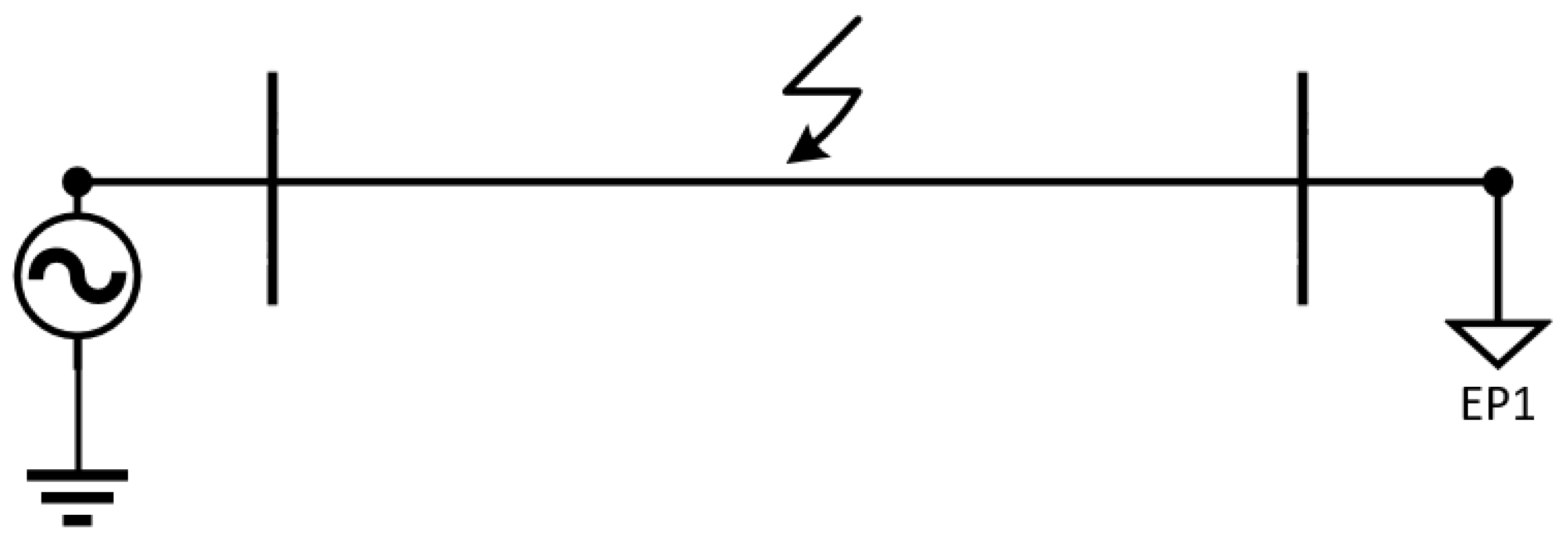
3.1. Single-Bus Transmission System

The single-line diagram of the power system used in this study is shown in Figure 2. The generator is represented by an equivalent potential source. The transmission line is represented using the Bergeron line model in PSCAD/EMTDC. The load is represented by an ohmic–inductive load [59]. The accuracy of classification depends on the number of data used for training and testing. Therefore, it is necessary to prepare large numbers of data for different faults and system conditions. The PSCAD software (PSCAD V5FREE) allows the creation of large sets of data using the multi-run component. In PSCAD, data are obtained for different situations by using the fault resistance and the fault onset angle. These data are presented to the user in the form of an output file from PSCAD [60].

3.2. IEEE 39-Busbar System

The IEEE 39-bus distribution system is a distribution system in the New England region of the United States. The system consists of 10 generators, 39 busbars, 12 transformers, 34 transmission lines, and 19 load points. The total power for the base configuration consists of 6145.97 MW active and 1363.41 MVAR reactive power [61,62]. The topology of the IEEE 39-bus distribution network is presented in Figure 3.

4. Results and Discussion

In this study, we first created the RTDS IEEE 39-bus model. Then, we created 11 fault conditions for different fault impedance values [63]. We achieved this with the RSCAD simulation program running on the RTDS simulator [64,65]. In the IEEE 39-bus system, fault detection can be performed by taking data from only eight different busbars. For this purpose, data were prepared by measuring the current and voltage values from each phase of eight different busbars (n = 3, 8, 11, 16, 20, 23, 29, 37). Outliers at different ratios were added to the fault data sets obtained from the IEEE 39-bus, and the response of the proposed method to outliers and noise was examined. Firstly, we added outliers at 0%, 5%, 10%, 15%, …, 50% and random samples were taken. Then, outliers were generated by preprocessing the target output. Next, based on the prepared data set, the accuracy of the CNN, LSTM, SVM, ELM, RVFLNs, Cauchy-M-RVFLN, and proposed methods was compared in the context of fault type and location detection.

In this study, new data sets were created by adding outliers to the data previously prepared in the RTDS as described. According to this data set, the fault type classification accuracy results for the ORR-RVFLN method are as given in Figure 4 and Figure 5. As can be seen in Figure 4 and Figure 5, very close results are found for the classification accuracy of different types of faults for different fault impedances using noise-free and noisy data. In the noisy case, the accuracy of the method used decreases by approximately 4% to 10%. However, even when noisy data are added, the proposed method achieves a high rate of success. According to the results, it is observed that the proposed method gives correct results despite the noise.

In light of the parameters given in this model, data were obtained for different fault impedances. The distances of the short circuits to the busbar were divided into seven different categories (0–50 m, 50–100 m, 100–150 m, 150–200 m, 250–300 m, 350–400 m, and >400 m), the smallest of which was between 0 and 50 m and the largest of which was more than 400 m. For each distance category, one hundred short circuits were simulated for different fault impedances and data were collected. Using the received data, the fault location was determined for four different fault impedances for each distance category with and without noise added. The fault location in the obtained data was determined by the ORR-RVFLN method.

Table 2. Comparison of fault location performance of different methods for a single 1 ph-g.

	With Noise	Without Noise	With Noise	Without Noise	With Noise	Without Noise	With Noise	Without Noise
ORR-RVFLN	0 ohm		30 ohm		50 ohm		100 ohm
0–50 m	61	59	63	60	66	62	69	65
>400 m	0	1	4	5	7	9	10	14
Cauchy-M-RVFLN	0 ohm		30 ohm		50 ohm		100 ohm
0–50 m	64	62	66	63	69	65	72	68
>400 m	3	4	6	7	9	11	12	16
RVFLN	0 ohm		30 ohm		50 ohm		100 ohm
0–50 m	66	64	68	65	71	67	73	69
>400 m	5	5	8	9	11	13	14	18
CNN	0 ohm		30 ohm		50 ohm		100 ohm
0–50 m	69	67	71	68	74	70	76	72
>400 m	6	7	9	10	12	14	15	19
LSTM	0 ohm		30 ohm		50 ohm		100 ohm
0–50 m	70	67	71	68	74	70	77	73
>400 m	7	7	10	11	13	15	16	20
SVM	0 ohm		30 ohm		50 ohm		100 ohm
0–50 m	70	68	72	69	75	71	78	73
>400 m	8	8	11	12	14	16	17	21
ELM	0 ohm		30 ohm		50 ohm		100 ohm
0–50 m	72	70	73	70	76	72	79	75
>400 m	10	11	14	15	17	19	20	24

shows the comparison of the ORR-RVFLN, Cauchy-M-RVFLN, RVFLN, CNN, LSTM, SVM, and ELM methods for single-phase ground fault location in the IEEE 39-bar system for distances between 0 and 50 m and greater than 400 m. This comparison was performed on both noisy and noiseless data for fault impedance values of 0 ohm, 30 ohm, 50 ohm, and 100 ohm. Table 2 shows that the fault location accuracy of the methods used was in the order of ORR-RVFLN, Cauchy-M-RVFLN, RVFLN, CNN, LSTM, SVM, and ELM. It is seen that the number of incorrect fault location predictions in the noise-added data is higher than for the noise-free data. The ORR-RVFLN method predicts the correct fault location more than the other methods. The ORR-RVFLN method makes 69 incorrect predictions for 100 faults between 0 and 50 m in the noise-added data with a fault impedance of 100 ohms, where the most incorrect fault locations are measured, while this value is 72 for the Cauchy-M-RVFLN method and 73 for the RVFLN method. The ORR-RVFLN method’s performance for 700 faults with and without noise added, for each fault impedance and for a single-phase ground fault, is also evaluated. At a 0 ohm fault impedance, the average distance error for 700 faults with noise added is 5.68 m. At a 100 ohm fault impedance, the average distance error with noise added is 14.42 m. In addition, the misestimated distance error increases as the fault impedance increases. The average fault distance error is higher in the data without added noise.

Table 3. Comparison of fault location performance of different methods for a single 2 ph-g.

	With Noise	Without Noise	With Noise	Without Noise	With Noise	Without Noise	With Noise	Without Noise
ORR-RVFLN	0 ohm		30 ohm		50 ohm		100 ohm
0–50 m	51	49	54	50	57	53	49	56
>400 m	0	0	1	2	2	4	5	6
Cauchy- M-RVFLN	0 ohm		30 ohm		50 ohm		100 ohm
0–50 m	52	53	58	51	58	54	50	56
>400 m	1	1	2	3	3	5	6	7
RVFLN	0 ohm		30 ohm		50 ohm		100 ohm
0–50 m	53	51	56	52	59	55	51	57
>400 m	2	2	3	4	4	6	7	7
CNN	0 ohm		30 ohm		50 ohm		100 ohm
0–50 m	57	55	59	55	62	58	54	61
>400 m	3	3	4	5	5	6	7	8
LSTM	0 ohm		30 ohm		50 ohm		100 ohm
0–50 m	57	55	60	56	63	59	55	61
>400 m	4	4	5	6	6	8	8	9
SVM	0 ohm		30 ohm		50 ohm		100 ohm
0–50 m	58	56	61	56	63	59	55	61
>400 m	8	8	9	10	10	12	13	14
ELM	0 ohm		30 ohm		50 ohm		100 ohm
0–50 m	59	57	62	58	65	61	57	64
>400 m	7	7	8	9	9	11	12	12

clearly demonstrates the superiority of the Cauchy-M-RVFLN, ORR-RVFLN, RVFLN, CNN, LSTM, SVM, and ELM methods over a range of fault conditions in the IEEE 39-bar system. Despite the presence of noise, these methods still outperform other techniques in terms of their fault location accuracy. Specifically, the table shows that the number of incorrect fault location estimates is higher for noisy data than for noiseless data. The ORR-RVFLN method is the most accurate in estimating the fault location, with only 49 incorrect predictions out of 100 faults between 0 and 50 m in noise-added data with a fault impedance of 100 ohms. In comparison, the Cauchy-M-RVFLN method has 50 incorrect predictions and the RVFLN method has 51. Furthermore, the average distance error for the ORR-RVFLN method is only 16.2 m for a fault impedance value of 100 ohms. The Cauchy-M-RVFLN method achieves an average distance error of 16.9 m for a fault impedance of 100 ohms, demonstrating its superior performance compared to the RVFLN method, which has an average distance error of 17.9 m.

Table 4. Comparison of fault location performance of different methods for a single 2 ph.

	With Noise	Without Noise	With Noise	Without Noise	With Noise	Without Noise	With Noise	Without Noise
ORR-RVFLN	0 ohm		30 ohm		50 ohm		100 ohm
0–50 m	55	53	58	56	61	58	63	59
>400 m	0	0	2	3	4	6	8	9
Cauchy-M-RVFLN	0 ohm		30 ohm		50 ohm		100 ohm
0–50 m	57	55	60	58	63	59	64	60
>400 m	2	2	4	5	6	8	9	10
RVFLN	0 ohm		30 ohm		50 ohm		100 ohm
0–50 m	58	56	61	59	64	61	66	62
>400 m	3	3	5	6	6	8	10	11
CNN	0 ohm		30 ohm		50 ohm		100 ohm
0–50 m	61	59	64	62	67	64	69	65
>400 m	4	4	6	7	8	9	11	12
LSTM	0 ohm		30 ohm		50 ohm		100 ohm
0–50 m	62	60	65	63	68	64	69	65
400 m	5	5	7	8	9	10	12	13
SVM	0 ohm		30 ohm		50 ohm		100 ohm
0–50 m	63	60	65	63	68	65	70	66
>400 m	6	6	8	9	10	11	13	14
ELM	0 ohm		30 ohm		50 ohm		100 ohm
0–50 m	64	62	67	65	70	66	71	67
>400 m	8	8	10	11	12	14	16	17

shows the comparison of the ORR-RVFLN, Cauchy-M-RVFLN, RVFLN, CNN, LSTM, SVM, and ELM methods for phase-to-phase fault location in the IEEE 39-bar system for distances between 0 and 50 m and greater than 400 m. This comparison was performed on both noisy and noiseless data for fault impedance values of 0 ohms, 30 ohms, 50 ohms, and 100 ohms. A careful examination of Table 4 shows that the number of incorrect fault location estimates is higher for noisy data than for noiseless data. The ORR-RVFLN method estimates more correct fault locations than the other methods. While the ORR-RVFLN method makes 63 incorrect predictions for 100 faults between 0 and 50 m in noise-added data with a fault impedance of 100 ohms, where the most incorrect fault locations are measured, this value is 64 for the Cauchy-M-RVFLN method and 66 for the RVFLN method. Additionally, the average distance error for ORR-RVFLN is 19.5 m for a 50 ohm fault impedance. For the Cauchy-M-RVFLN method, the average distance error is 20.7 m for a fault impedance of 50 ohms and 22.2 m for the RVFLN method.

Table 5. Comparison of fault location performance of different methods for a single 3 ph.

	With Noise	Without Noise	With Noise	Without Noise	With Noise	Without Noise	With Noise	Without Noise
ORR-RVFLN	0 ohm		30 ohm		50 ohm		100 ohm
0–50 m	58	57	60	59	62	60	65	61
>400 m	0	1	3	4	5	8	9	12
Cauchy-M-RVFLN	0 ohm		30 ohm		50 ohm		100 ohm
0–50 m	61	60	63	61	64	62	67	63
>400 m	2	3	5	6	7	10	11	14
RVFLN	0 ohm		30 ohm		50 ohm		100 ohm
0–50 m	62	61	64	63	66	64	68	64
>400 m	4	5	7	7	8	11	12	15
CNN	0 ohm		30 ohm		50 ohm		100 ohm
0–50 m	65	64	67	66	69	67	72	68
>400 m	5	6	8	8	9	12	13	16
LSTM	0 ohm		30 ohm		50 ohm		100 ohm
0–50 m	66	65	68	66	69	67	72	68
>400 m	6	7	9	9	10	13	14	17
SVM	0 ohm		30 ohm		50 ohm		100 ohm
0–50 m	66	65	68	67	70	68	73	69
>400 m	7	8	10	10	11	14	15	18
ELM	0 ohm		30 ohm		50 ohm		100 ohm
0–50 m	68	67	70	69	71	69	74	70
>400 m	9	10	12	13	14	17	18	21

presents a comparison of various methods, including ORR-RVFLN, Cauchy-M-RVFLN, RVFLN, CNN, LSTM, SVM, and ELM, for three-phase fault localization in the IEEE 39-bar system. The comparison takes into account distances ranging from 0 to 50 m and greater than 400 m, as well as both noisy and noiseless data. Additionally, fault impedance values of 0 ohm, 30 ohm, 50 ohm, and 100 ohm are considered. According to the data presented in Table 5, various methods, including ORR-RVFLN, Cauchy-M-RVFLN, RVFLN, CNN, LSTM, SVM, and ELM, exhibited good fault location accuracy. It is worth noting that the number of faulty fault location predictions in the noise-added data is higher than in the noise-free data. Additionally, the ORR-RVFLN method is found to outperform the other methods in predicting the correct fault location. In the noise-added data with a fault impedance of 100 ohms, the ORR-RVFLN method produces 65 incorrect predictions out of 100 faults between 0 and 50 m, while measuring the most faulty fault locations. The Cauchy-M-RVFLN method produces 67 incorrect predictions and the RVFLN method produces 68. Moreover, when the fault impedance value is 30 ohms, the average distance error for the ORR-RVFLN method is 18.9 m. According to the analysis, it appears that the Cauchy-M-RVFLN method has an average distance error of 20.6 m when the fault impedance value is 30 ohms. On the other hand, the RVFLN method has an average distance error of 21.9 m when the data have added noise.

5. Conclusions

In this paper, in the IEEE 39-busbar power system modeled in the RTDS, with 0 ohm, 10 ohm, 50 ohm, and 100 ohm fault short circuits, was studied for three single-phase ground faults, three two-phase ground faults, three phase-phase faults, and one three-phase short-circuit fault. In addition, random noise was added to make the data closer to reality. The ORR-RVFLN method is presented to detect short-circuit faults of different resistances and types. For this purpose, RSCAD, was used to simulate real systems. The IEEE 39-busbar system was used for fault type and fault location detection. Unlike the existing studies in the literature, six new feature vectors were developed in this work to be used in fault detection. It was observed that the developed feature vectors increased the fault detection accuracy of the proposed methods. It was found that the six new feature vectors contributed to increasing the detection accuracy of high-impedance short-circuit faults by approximately 10%. An important issue in fault location detection is to detect fault locations that occur at long distances from the busbar with high accuracy. In the category where the distance was greater than 400 m, the number of faulty detections under the same conditions was 10 for single-phase ground faults, nine for three-phase faults, eight for phase-phase faults, and five for two-phase ground faults. These results show that the method correctly detects the fault location at distances greater than 400 m with over 90% accuracy.

The ORR-RVFLN method is proposed for fault location. When the obtained results are analyzed, it is found that the number of incorrect fault locations increases as the fault impedance increases and decreases as the distance to the busbar increases. This general trend is valid for all fault types. For all fault types, the number of incorrect fault locations and the average distance errors were obtained in seven categories of 0–50, 50–100, 100–150, 150–200, 250–300, 350–400, and >400 m distances from the busbar. For each distance category, 100 different faults were created, and it was investigated whether these faults were correctly located in each category. The highest number of faulty locations was observed in the 0–50 m range, which represented the closest distance to the busbar. At a fault impedance of 100 ohms, the number of faulty detections in this range was 69 for single-phase-ground faults, 65 for three-phase faults, 63 for phase-phase faults, and 49 for two-phase-ground faults using noisy data. The performance of the ORR-RVFLN, Cauchy-M-RVFLN, RVFLN, CNN, LSTM, SVM, and ELM methods was compared for fault location. At the end of this comparison, it was found that the ORR-RVFLN method showed the best performance, followed by the Cauchy-M-RVFLN, RVFLN, CNN, LSTM, SVM, and ELM methods, respectively. The ORR-RVFLN method predicted the single-phase ground faults about 10% better than the ELM method, which was the worst method, and about 3% better than the Cauchy-M-RVFLN method, which was the closest method. Similar results were obtained for other fault types. In addition, in this study, the average detection success rate of the ORR-RVFLN method was 92.2% for all fault impedances with noise added to the data.

References

1. Jordehi, A.R. Optimisation of electric distribution systems: A review. Renew. Sustain. Energy Rev. 2015, 51, 1088–1100. [Google Scholar] [CrossRef]
2. Rezapour, H.; Jamali, S.; Siano, P. Wide-Area Protection System for Radial Smart Distribution Networks. Appl. Sci. 2024, 14, 4862. [Google Scholar] [CrossRef]
3. Silos-Sanchez, A.; Villafafila-Robles, R.; Lloret-Gallego, P. Novel fault location algorithm for meshed distribution networks with DERs. Electr. Power Syst. Res. 2020, 181, 106182. [Google Scholar] [CrossRef]
4. Nsaif, Y.M.; Lipu, M.H.; Ayob, A.; Yusof, Y.; Hussain, A. Fault detection and protection schemes for distributed generation integrated to distribution network: Challenges and suggestions. IEEE Access 2021, 9, 142693–142717. [Google Scholar] [CrossRef]
5. Zeng, Y.; Jiang, S.; Konstantinou, G.; Pou, J.; Zou, G.; Zhang, X. Multi-Objective Controller Design for Grid-Following Converters with Easy Transfer Reinforcement Learning. IEEE Trans. Power Electron. 2025, in press. [Google Scholar] [CrossRef]
6. Zeng, Y.; Xiao, Z.; Liu, Q.; Liang, G.; Rodriguez, E.; Zou, G.; Zhang, X.; Pou, J. Physics-informed deep transfer reinforcement learning method for the input-series output-parallel dual active bridge-based auxiliary power modules in electrical aircraft. IEEE Trans. Transp. Electrif. 2024, in press. [Google Scholar] [CrossRef]
7. Haydaroğlu, C.; Yıldırım, B.; Kılıç, H.; Özdemir, M.T. The Effect of Local and Interarea Oscillations of Wind Turbine Generators Based on Permanent Magnet Synchronous Generators Connected to a Power System. Turk. J. Electr. Power Energy Syst. 2024. [Google Scholar] [CrossRef]
8. Gholami, M.; Abbaspour, A.; Moeini-Aghtaie, M.; Fotuhi-Firuzabad, M.; Lehtonen, M. Detecting the location of short-circuit faults in active distribution network using PMU-based state estimation. IEEE Trans. Smart Grid 2019, 11, 1396–1406. [Google Scholar] [CrossRef]
9. Çetin, M.S.; Gençoğlu, M.T.; Şahin, H. A Review of Electric Vehicles: Their Impact on The Electricity Grid and Artificial Intelligence-Based Approaches for Charging Load Management. Int. J. Energy Smart Grid 2024, 9, 51–59. [Google Scholar] [CrossRef]
10. Regional Group Nordic. Nordic and Baltic Grid Disturbance Statistics 2020; Regional Group Nordic: Copenhagen, Denmark, 2020. [Google Scholar]
11. Lale, T.; Yüksek, G. Identification and Classification of Turn ShortCircuit and Demagnetization Failures in PMSM Using LSTM and GRU Methods. Bull. Pol. Acad. Sci. Tech. Sci. 2024, e15158. [Google Scholar]
12. Zeng, X.; Gao, W.; Yang, G. High impedance fault detection in distribution network based on S-transform and average singular entropy. Glob. Energy Interconnect. 2023, 6, 64–80. [Google Scholar] [CrossRef]
13. Gururajapathy, S.S.; Mokhlis, H.; Illias, H.A. Fault location and detection techniques in power distribution systems with distributed generation: A review. Renew. Sustain. Energy Rev. 2017, 74, 949–958. [Google Scholar] [CrossRef]
14. Aleem, S.A.; Shahid, N.; Naqvi, I.H. Methodologies in power systems fault detection and diagnosis. Energy Syst. 2015, 6, 85–108. [Google Scholar] [CrossRef]
15. Chen, Y.Q.; Fink, O.; Sansavini, G. Combined fault location and classification for power transmission lines fault diagnosis with integrated feature extraction. IEEE Trans. Ind. Electron. 2017, 65, 561–569. [Google Scholar] [CrossRef]
16. Mohammadi, A.; Jannati, M.; Shams, M. Using deep transfer learning technique to protect electrical distribution systems against high-impedance faults. IEEE Syst. J. 2023, 17, 3160–3171. [Google Scholar] [CrossRef]
17. Sangeeth, B.K.; Vinod, V. High impedance fault detection using multi-domain feature with artificial neural network. Electr. Power Components Syst. 2023, 51, 366–379. [Google Scholar] [CrossRef]
18. Baharozu, E.; Ilhan, S.; Soykan, G. High impedance fault localization: A comprehensive review. Electr. Power Syst. Res. 2023, 214, 108892. [Google Scholar] [CrossRef]
19. Lopes, G.N.; Menezes, T.S.; Gomes, D.P.; Vieira, J.C.M. High Impedance Fault Location Methods: Review and Harmonic Selection-based Analysis. IEEE Open Access J. Power Energy 2023, 10, 438–449. [Google Scholar] [CrossRef]
20. Hamatwi, E.; Imoru, O.; Kanime, M.M.; Kanelombe, H.S. Comparative Analysis of High Impedance Fault Detection Techniques on Distribution Networks. IEEE Access 2023, 11, 25817–25834. [Google Scholar] [CrossRef]
21. Thomas, J.B.; Chaudhari, S.G.; Shihabudheen, K.; Verma, N.K. CNN-based transformer model for fault detection in power system networks. IEEE Trans. Instrum. Meas. 2023, 72, 2504210. [Google Scholar] [CrossRef]
22. Lingampalli, B.R.; Rao, K.S. Validation of Passive Islanding Detection Methods for Double Line-to-Ground Unsymmetrical Fault in a Three-Phase Microgrid System. Turk. J. Electr. Power Energy Syst. 2022, 2, 11–20. [Google Scholar] [CrossRef]
23. Ola, S.R.; Saraswat, A.; Goyal, S.K.; Jhajharia, S.; Rathore, B.; Mahela, O.P. Wigner distribution function and alienation coefficient-based transmission line protection scheme. IET Gener. Transm. Distrib. 2020, 14, 1842–1853. [Google Scholar] [CrossRef]
24. Abasi, M.; Sadeghian, O. A ground fault location algorithm in double-circuit transmission lines with T-off connection to an industrial microgrid by using current and voltage phasors information of a single terminal. IET Gener. Transm. Distrib. 2024, 18, 1714–1741. [Google Scholar] [CrossRef]
25. Mamuya, Y.D.; Lee, Y.D.; Shen, J.W.; Shafiullah, M.; Kuo, C.C. Application of machine learning for fault classification and location in a radial distribution grid. Appl. Sci. 2020, 10, 4965. [Google Scholar] [CrossRef]
26. Sowah, R.A.; Dzabeng, N.A.; Ofoli, A.R.; Acakpovi, A.; Koumadi, K.M.; Ocrah, J.; Martin, D. Design of power distribution network fault data collector for fault detection, location and classification using machine learning. In Proceedings of the 2018 IEEE 7th International Conference on Adaptive Science &Technology (ICAST), Accra, Ghana, 22–24 August 2018; pp. 1–8. [Google Scholar]
27. Rathore, B.; Mahela, O.P.; Khan, B.; Alhelou, H.H.; Siano, P. Wavelet-alienation-neural-based protection scheme for STATCOM compensated transmission line. IEEE Trans. Ind. Informatics 2020, 17, 2557–2565. [Google Scholar] [CrossRef]
28. Rathore, B.; Shaik, A.G. Wavelet-alienation based transmission line protection scheme. IET Gener. Transm. Distrib. 2017, 11, 995–1003. [Google Scholar] [CrossRef]
29. Yadav, A.; Swetapadma, A. Enhancing the performance of transmission line directional relaying, fault classification and fault location schemes using fuzzy inference system. IET Gener. Transm. Distrib. 2015, 9, 580–591. [Google Scholar] [CrossRef]
30. Ravesh, N.R.; Ramezani, N.; Ahmadi, I.; Nouri, H. A hybrid artificial neural network and wavelet packet transform approach for fault location in hybrid transmission lines. Electr. Power Syst. Res. 2022, 204, 107721. [Google Scholar] [CrossRef]
31. Gopakumar, P.; Reddy, M.J.B.; Mohanta, D.K. Adaptive fault identification and classification methodology for smart power grids using synchronous phasor angle measurements. IET Gener. Transm. Distrib. 2015, 9, 133–145. [Google Scholar] [CrossRef]
32. Shi, S.; Zhu, B.; Mirsaeidi, S.; Dong, X. Fault classification for transmission lines based on group sparse representation. IEEE Trans. Smart Grid 2018, 10, 4673–4682. [Google Scholar] [CrossRef]
33. Ghaemi, A.; Safari, A.; Afsharirad, H.; Shayeghi, H. Accuracy enhance of fault classification and location in a smart distribution network based on stacked ensemble learning. Electr. Power Syst. Res. 2022, 205, 107766. [Google Scholar] [CrossRef]
34. Gangwar, A.K.; Mahela, O.P.; Rathore, B.; Khan, B.; Alhelou, H.H.; Siano, P. A Novel k-Means Clustering and Weighted k-NN-Regression-Based Fast Transmission Line Protection. IEEE Trans. Ind. Informatics 2020, 17, 6034–6043. [Google Scholar] [CrossRef]
35. Ananthan, S.N.; Padmanabhan, R.; Meyur, R.; Mallikarjuna, B.; Reddy, M.J.B.; Mohanta, D.K. Real-time fault analysis of transmission lines using wavelet multi-resolution analysis based frequency-domain approach. IET Sci. Meas. Technol. 2016, 10, 693–703. [Google Scholar] [CrossRef]
36. Salehi, M.; Namdari, F. Fault classification and faulted phase selection for transmission line using morphological edge detection filter. IET Gener. Transm. Distrib. 2018, 12, 1595–1605. [Google Scholar] [CrossRef]
37. Zhang, H.Y.; Xie, Y.Z.; Yi, T.Q.; Kong, X.; Cheng, L.; Liu, H.J. Fault Detection for High-Voltage Circuit Breakers Based on Time–Frequency Analysis of Switching Transient E-Fields. IEEE Trans. Instrum. Meas. 2019, 69, 1620–1631. [Google Scholar] [CrossRef]
38. Taheri, B.; Salehimehr, S.; Sedighizadeh, M. A novel strategy for fault location in shunt-compensated double circuit transmission lines equipped by wind farms based on long short-term memory. Clean. Eng. Technol. 2022, 6, 100406. [Google Scholar] [CrossRef]
39. Hu, J.; Hu, W.; Chen, J.; Cao, D.; Zhang, Z.; Liu, Z.; Chen, Z.; Blaabjerg, F. Fault Location and Classification for Distribution Systems Based on Deep Graph Learning Methods. J. Mod. Power Syst. Clean Energy 2022, 11, 35–51. [Google Scholar] [CrossRef]
40. Ding, C.; Ma, P.; Jiang, C.; Wang, F. Fast Fault Line Selection Technology of Distribution Network Based on MCECA-CloFormer. Appl. Sci. 2024, 14, 8270. [Google Scholar] [CrossRef]
41. Sodin, D.; Rudež, U.; Mihelin, M.; Smolnikar, M.; Čampa, A. Advanced edge-cloud computing framework for automated pmu-based fault localization in distribution networks. Appl. Sci. 2021, 11, 3100. [Google Scholar] [CrossRef]
42. Wan, Q.; Li, Y.; Yuan, R.; Meng, Q.; Li, X. Fault Identification and Localization of a Time- Frequency Domain Joint Impedance Spectrum of Cables Based on Deep Belief Networks. Sensors 2023, 23, 684. [Google Scholar] [CrossRef] [PubMed]
43. Xu, S.; Ouyang, J.; Chen, J.; Xiong, X. A Section Location Method of Single-Phase Short-Circuit Faults for Distribution Networks Containing Distributed Generators Based on Fusion Fault Confidence of Short-Circuit Current Vectors. Electronics 2024, 13, 1741. [Google Scholar] [CrossRef]
44. Majidi, M.; Fadali, M.S.; Etezadi-Amoli, M.; Oskuoee, M. Partial discharge pattern recognition via sparse representation and ANN. IEEE Trans. Dielectr. Electr. Insul. 2015, 22, 1061–1070. [Google Scholar] [CrossRef]
45. Pao, Y.H.; Takefuji, Y. Functional-link net computing: Theory, system architecture, and functionalities. Computer 1992, 25, 76–79. [Google Scholar] [CrossRef]
46. Pao, Y.H.; Park, G.H.; Sobajic, D.J. Learning and generalization characteristics of the random vector functional-link net. Neurocomputing 1994, 6, 163–180. [Google Scholar] [CrossRef]
47. Igelnik, B.; Pao, Y.H. Stochastic choice of basis functions in adaptive function approximation and the functional-link net. IEEE Trans. Neural Netw. 1995, 6, 1320–1329. [Google Scholar] [CrossRef]
48. Zhou, P.; Lv, Y.; Wang, H.; Chai, T. Data-driven robust RVFLNs modeling of a blast furnace iron-making process using Cauchy distribution weighted M-estimation. IEEE Trans. Ind. Electron. 2017, 64, 7141–7151. [Google Scholar] [CrossRef]
49. Haydaroğlu, C.; Gümüş, B. Fault Detection in Distribution Network with the Cauchy-M Estimate—RVFLN Method. Energies 2022, 16, 252. [Google Scholar] [CrossRef]
50. Kilic, H.; Gumus, B.; Yilmaz, M. Fault detection in photovoltaic arrays: A robust regularized machine learning approach. DYNA-Ing. E Ind. 2020, 95, 622–628. [Google Scholar] [CrossRef] [PubMed]
51. Kiliç, H.; Gumus, B.; Khaki, B.; Yilmaz, M.; Palensky, P.; Authority, P. A Robust Data-Driven Approach for Fault Detection in Photovoltaic Arrays. In Proceedings of the 10th IEEE PES Innovative Smart Grid Technologies Europe, ISGT-Europe, Virtual, 26–28 October 2020. [Google Scholar]
52. Eryılmaz, B.; Kılıç, H.; Koçyiğit, F. Makine Öğrenimi Tabanlı Kısa Vadeli Fotovoltaik Çıkış Gücü Tahminlemesi. EMO Bilimsel Dergi 2023, 13, 57–69. [Google Scholar]
53. Dai, W.; Chen, Q.; Chu, F.; Ma, X.; Chai, T. Robust regularized random vector functional link network and its industrial application. IEEE Access 2017, 5, 16162–16172. [Google Scholar] [CrossRef]
54. Li, M.; Wang, D. Insights into randomized algorithms for neural networks: Practical issues and common pitfalls. Inf. Sci. 2017, 382, 170–178. [Google Scholar] [CrossRef]
55. Hoerl, A.E.; Kennard, R.W. Ridge regression: Biased estimation for nonorthogonal problems. Technometrics 1970, 12, 55–67. [Google Scholar] [CrossRef]
56. Huynh, H.T.; Won, Y. Regularized online sequential learning algorithm for single-hidden layer feedforward neural networks. Pattern Recognit. Lett. 2011, 32, 1930–1935. [Google Scholar] [CrossRef]
57. Scott, D.W. Multivariate Density Estimation: Theory, Practice, and Visualization; John Wiley & Sons: Hoboken, NJ, USA, 2015. [Google Scholar]
58. Hansen, P.C. Rank-Deficient and Discrete Ill-Posed Problems: Numerical Aspects of Linear Inversion; SIAM: Philadelphia, PA, USA, 1998. [Google Scholar]
59. Gümüs, B.; Kılıç, H.; Haydaroglu, C.; Butakın, U.Y. Fault type and fault location detection in transmission lines with 6-convolutional layered CNN. Bull. Pol. Acad. Sci. Tech. Sci. 2024, 72. [Google Scholar] [CrossRef]
60. Nascimento, A.L.; Yahyaoui, I.; Fardin, J.F.; Encarnação, L.F.; Tadeo, F. Modeling and experimental validation of a PEM fuel cell in steady and transient regimes using PSCAD/EMTDC software. Int. J. Hydrog. Energy 2020, 45, 30870–30881. [Google Scholar] [CrossRef]
61. Athay, T.; Podmore, R.; Virmani, S. A Practical Method for the Direct Analysis of Transient Stability. IEEE Trans. Power Appar. Syst. 1979, PAS-98, 573–584. [Google Scholar] [CrossRef]
62. Cupelli, M.; Doig Cardet, C.; Monti, A. Voltage stability indices comparison on the IEEE-39 bus system using RTDS. In Proceedings of the 2012 IEEE International Conference on Power System Technology (POWERCON), Auckland, New Zealand, 30 October–2 November 2012; pp. 1–6. [Google Scholar] [CrossRef]
63. Montoya, J.; Brandl, R.; Vishwanath, K.; Johnson, J.; Darbali-Zamora, R.; Summers, A.; Hashimoto, J.; Kikusato, H.; Ustun, T.S.; Ninad, N.; et al. Advanced laboratory testing methods using real-time simulation and hardware-in-the-loop techniques: A survey of smart grid international research facility network activities. Energies 2020, 13, 3267. [Google Scholar] [CrossRef]
64. Sidwall, K.; Forsyth, P. Advancements in real-time simulation for the validation of grid modernization technologies. Energies 2020, 13, 4036. [Google Scholar] [CrossRef]
65. Dash, P.K.; Das, S.; Moirangthem, J. Distance protection of shunt compensated transmission line using a sparse S-transform. IET Gener. Transm. Distrib. 2015, 9, 1264–1274. [Google Scholar] [CrossRef]
Figure 1. RVFLN algorithm.
Applsci 15 01908 g001
Figure 2. Single-busbar transmission line model.
Applsci 15 01908 g002
Figure 3. IEEE 39-busbar model.
Applsci 15 01908 g003
Figure 4. ORR-RVFLN detection rate on data with no noise added.
Applsci 15 01908 g004
Figure 5. ORR-RVFLN detection rate on data with procedural noise.
Applsci 15 01908 g005