Multi-Scale Twin Networks for Coastal Zone Change Detection in Remote Sensing Imagery

Abstract

Accurate coastal zone change detection is crucial for coastal urban planning and marine resource development. To address the specificity of coastal zone change detection and the category imbalance issue in the model, we propose a multi-scale coastal zone change detection method (AMMNet) based on the attention mechanism. The method leverages multi-scale features extracted by the ResNet backbone, which are then optimized and integrated through high-frequency attention and spatio-temporal difference modules. These modules allow the model to focus on both global and local changes, enhancing its ability to detect variations in coastal zones. Additionally, the foreground attention module refines the model’s attention on relevant regions, ensuring improved performance. The experimental results show that our method achieves the highest scores in several evaluation metrics, demonstrating significant advantages in accuracy and generalization and effectively addressing the category imbalance problem. It provides a robust solution for coastal zone change detection.

1. Introduction

The coastal zone is broadly defined as the area extending from the coastline into both land and sea, encompassing coastal plains, wetlands, estuarine deltas, tidal zones, submerged slopes, and the shallow continental shelf [1]. This region features a unique ecosystem, high biological productivity, and significant economic value [2]. Due to its favorable natural conditions and frequent human activities, the coastal zone undergoes rapid and diverse changes, primarily manifested as coastal erosion and sedimentation, sea-level rise, wetland degradation, vegetation cover loss, and land-use changes. These transformations lead to constant alterations in the geomorphological characteristics of the coastal zone: erosion causes the coastline to retreat, sedimentation pushes it forward, rising sea levels inundate low-lying areas, fluctuations in vegetation lead to frequent changes in the water environment, and human development activities drive land-use changes. Driven by these five key factors, the area of coastal wetlands decreases, biodiversity declines, and both vegetation types and density decrease, which ultimately disrupts ecological balance. Therefore, studying coastal zone changes and monitoring their trends is crucial for development planning and regulatory governance [1].

Since the concept of automated change detection was first introduced in the 1960s [3], advances in remote sensing technology have driven significant progress in change detection techniques [4].Remote sensing imagery allows researchers to acquire large-scale, continuous spatio-temporal data, making it particularly effective for monitoring island areas that are difficult to access directly [5]. Not only does remote sensing imagery provide direct evidence of changes in the coastal zone, but it also enables data analysis to reveal patterns and trends in these changes [6]. However, the expansion of image data increases the imbalance between change and non-change samples, leading to a category imbalance problem. This imbalance makes it difficult for change detection models to accurately identify changes in minority categories, thereby negatively affecting overall detection accuracy. Therefore, how to effectively address the class imbalance and improve the model’s performance in complex scenarios has become an important challenge that current change detection techniques urgently need to solve.

Unlike changes in terrestrial buildings, coastal zone changes are characterized by low color differentiation between changed and unchanged regions, along with irregular boundary shapes, making detection particularly challenging. Therefore, change detection methods must be capable of extracting and processing both global and local information [7]. Moreover, due to the frequent environmental changes in coastal zones, the demand for coastal zone change detection is primarily focused on short-term changes. The short time intervals between pre- and post-event images result in subtle changes and fewer samples, exacerbating the category imbalance problem in the dataset. Consequently, mitigating the impact of this imbalance on model accuracy is a critical issue we aim to address. Furthermore, there has been limited research on coastal zone change detection in recent years, both domestically and internationally, and the available public datasets contain very few samples of coastal zone area changes [8]. Therefore, given the unique characteristics of coastal zone changes and incorporating the recent advancements in change detection methods, designing a practical and accurate change detection approach for the coastal zone is another key challenge we seek to resolve.

To address these challenges, we propose a multi-scale coastal zone change detection method (AMMNet) that incorporates multiple attention mechanisms. By modularizing different attention mechanisms, each is tasked with extracting and integrating features at various scales. These modules work collaboratively to process complex coastal zone changes, ultimately generating a high-quality change detection map. This approach efficiently combines the strengths of each attention mechanism, ensuring improved performance and accurate results despite the challenges posed by the coastal environment.

The remainder of this paper is organized as follows. Section 2 reviews the related work on coastal zone change detection, highlighting the advances in deep learning methods and attention mechanisms. Section 3 introduces the proposed methodology, including the design and functioning of the AMMNet model and its core modules. Section 4 presents the datasets, experimental setup, and evaluation metrics, followed by a detailed discussion of the experimental results and comparisons with state-of-the-art methods. Section 5 concludes the study, summarizing the key contributions. Finally, Section 6 discusses the limitations of the proposed method and provides directions for future research.

2. Related Work

2.1. Deep Learning-Based Change Detection Method

In recent years, deep learning methods, with their powerful data processing capabilities and automatic feature extraction advantages, have achieved comparable results with simpler architectures [9]. However, due to the complexity of deep learning models and their reliance on large datasets, they are more significantly affected by the category imbalance problem. To address this, researchers have proposed various deep learning network architectures that better handle category imbalance, many of which are based on twin network structures. Twin networks use a pair of deep neural networks with shared weights to independently extract the key features from pre- and post-event remote sensing images. By analyzing the differences between these features, the networks identify areas of change and generate a map that highlights the detected changes [10]. For example, the DTCDSCN model proposed by Liu Y et al. [11] introduces a deep convolutional network with dual-task constraints, enabling simultaneous change detection and semantic segmentation. By using a shared feature extraction layer, it improves the discriminative power of the extracted features and resolves the issue of insufficient feature discrimination in traditional methods. Meanwhile, the MSCANet model proposed by Liu M et al. [12] combines the strengths of CNNs and transformers, capturing long-range dependencies via a multi-scale context aggregation module, which is particularly effective for detecting fine-grained changes in high-resolution remote sensing images. Liu W et al.’s [13] AMTNet introduces a multi-scale transformer-based attention mechanism to model spatio-temporal contextual information effectively. Additionally, it uses a feature exchange module to partially exchange features between different time domains, reducing inter-domain differences and improving change detection accuracy and robustness. The primary advantage of twin networks lies in their ability to effectively capture the similarities and differences between two images through shared weights, thereby improving detection accuracy. The shared and co-optimized parameters between the two branches also help reduce the risk of overfitting.

We hope that in the complex and changing coastal zone environment, different levels of useful features can be effectively combined to better capture the variability between pre- and post-images to improve the model’s ability to perceive complex changes. However, single-stream methods can suffer from feature confusion, information redundancy, and loss of spatial information due to the need to cascade together the pre- and post-image inputs, which affects the detection accuracy of the model. Therefore, we designed a multi-scale twin network using the idea of dual-stream methods. Multi-scale processing can effectively extract feature information at different levels to avoid the problem of information loss that may occur at a single scale, and the structure of the twin network allows the pre- and post-images to be processed separately through independent network branches, thus avoiding the problems of feature confusion and information redundancy. This design can retain the useful spatial information in the image more precisely, enhance the model’s perceptual ability in the face of complex changes, and ultimately improve the accuracy of detection.

2.2. DAttention Mechanism in CD

In the change detection task, the attention mechanism is increasingly used, which can automatically focus on the key features in the changed region while suppressing the interfering information in the unchanged region, thus enhancing the detection capability of the model. For example, the JoinAtt module in the dual-branch multi-level spatio-temporal network (DMINet) cleverly implements feature interactions to direct attention to the real change [14]. The DSIFN proposed by Zhang et al. [15] utilizes multi-scale features combined with an attention module to improve feature fusion. The SNUNet proposed by Fang et al. [16] improves the modeling capability of contextual information by integrating the channel attention modeling capability of contextual information, which makes the intermediate feature representation richer. To address the category imbalance problem, the MFPNet [17] introduces adaptive channel weights to better focus on changing regions. In addition, for the pixel-level long-distance dependency problem, some works try to model spatio-temporal contextual relationships through the self-attention mechanism, which achieves ideal results but faces the problem of rising computational complexity.

Therefore, we designed a high-frequency attention module (HFAM), which improves the detection accuracy of the edges of the change region by combining the two phases of spatial attention and high-frequency enhancement and effectively enhances the change detection performance of the model, and a spatio-temporal disparity attention module (SDAM), which learns the global change information of the bi-temporal features and the fine-grained local content, respectively, by adopting a dual-branching structure, utilizing the coordinates of the attention to capture the spatio-temporal differences while extracting local context information through cascading convolution, thus enhancing the representation of the change region and suppressing interference noise.

3. Principles and Methods

Our proposed AMMNet is a typical multi-scale twin network consisting of five components: ResNet, HFAM, the feature exchange module, the SDAM, and the classifier. ResNet serves as the backbone of the coastal zone change detection network, which is responsible for extracting multi-scale features from the dual-temporal input images. By removing the initial fully connected layers, it helps reduce information loss. The HFAM is designed to integrate multi-scale features, leveraging spatial attention and introducing the Sobel operator to selectively enhance the high-frequency information of buildings in the building change detection task. This enables the network to capture different levels of predictable coastal zone change patterns, improving the overall performance of complex coastal zone change detection while minimizing the interference of redundant information and irrelevant features. The feature exchange module merges multi-layered features, balancing both detail and semantic information, thus improving the model’s change detection capability while simplifying computation and optimizing gradient flow. The SDAM helps the model gradually focus on the change regions by integrating and processing feature maps at different scales, enhancing the learning of change information and alleviating the issue of category imbalance. Finally, the classifier generates the change result map by applying a thresholding mechanism.

As shown in Figure 1, let ${\mathrm{X}}_1\in {\mathrm{R}}^{3\times \mathrm{H}\times \mathrm{W}}$ and ${\mathrm{X}}_2\in {\mathrm{R}}^{3\times \mathrm{H}\times \mathrm{W}}$ denote the pre- and post-event remote sensing images of the same coastal zone area taken at different times. The change detection method follows the three steps outlined below:

Step 1 (edge feature extraction): The two images ${\mathrm{X}}_{\mathrm{i}}\left(\forall \mathrm{i}\in \left\{1,2\right\}\right)\in {\mathrm{R}}^{3\times \mathrm{H}\times \mathrm{W}}$ are passed through the ResNet backbone, and three feature maps at different scales ${\mathrm{F}}_{\mathrm{i}}^{1\left(1\right)}$, ${\mathrm{F}}_{\mathrm{i}}^{2\left(1\right)}$, and ${\mathrm{F}}_{\mathrm{i}}^{3\left(1\right)}\left(\forall \mathrm{i}\in \left\{1,2\right\}\right)$ are extracted from each image. These feature maps are then swapped with the feature maps of the same scale from the other branch of the twin.

Network to minimize the domain gap between images from different time periods. After the exchange, the feature maps ${\mathrm{F}}_{\mathrm{i}}^{\mathrm{j}\left(2\right)}\left(\forall \mathrm{j}\in \left\{1,2,3\right\},\forall \mathrm{i}\in \left\{1,2\right\}\right)$ are passed into the high-frequency attention module (HFAM), which integrates the commonly used spatial and channel attention mechanisms and introduces the Sobel operator in the channel attention to enhance the model’s feature extraction ability. This helps to obtain clearer edge features and improves the model’s sensitivity to rapidly changing regions (such as edges, textures, and details) in coastal zone change detection.

Step 2 (integration of contextual information): First, the three high-frequency feature maps ${\mathrm{F}}_{\mathrm{i}}^{\mathrm{j}\left(2\right)}$ from the same branch are rescaled to the same spatial scale. The feature maps at different scales are then fused using element-wise summation to obtain combined feature maps ${\mathrm{F}}_{\mathrm{i}}^{\mathrm{j}\left(3\right)}\left(\forall \mathrm{j}\in \left\{1,2,3\right\},\forall \mathrm{i}\in \left\{1,2\right\}\right)$, which facilitates the full utilization of both local detail and global contextual information. These two types of information complement each other, improving detection accuracy, especially at the boundaries of changing regions. Next, the feature maps from different branches, but at the same scale, are grouped into three pairs and passed into the spatio-temporal disparity attention module (SDAM) to obtain feature maps ${\mathrm{F}}^{\mathrm{i}\left(4\right)}\left(\forall \mathrm{i}\in \left\{1,2,3\right\}\right)$, which integrates both spatio-temporal global information and local contextual information through its dual-branch structure. This effectively enhances the representation of change-related regions while suppressing irrelevant interference.

Step 3 (change result generation): The feature map ${\mathrm{F}}^{\mathrm{i}\left(4\right)}$ is first passed into the foreground attention module (FAM), which strengthens the network’s ability to capture the foreground by analyzing the relationship between the background and foreground. This enables the change detection network to better integrate foreground-related contextual information and effectively delineate the boundaries of the change region, alleviating the imbalance problem. Finally, the feature map ${\mathrm{F}}^{\left(5\right)}$ is fed into the classifier, and the predicted change map is generated using a thresholding technique.

3.1. Edge Feature Extraction

We used ResNet as the backbone network, with the initial fully connected layer removed, consisting of five layers: one convolutional layer (Conv1) and four residual blocks (Res2, Res3, Res4, Res5). ResNet introduces residual connections, which mitigate the vanishing/explosion gradient problem and enhance the trainability of deep neural networks. In the coastal zone change detection task, ResNet can gradually extract and integrate features at multiple scales while preserving details through its deep structure and residual connections, which helps process complex information in high-resolution coastal zone images. The backbone network performs downsampling operations with a stride of 2 in Res3 and Res4, obtaining feature maps at different scales. Removing the initial fully connected layer prevents the loss of spatial information due to flattening the input image. Moreover, removing the fully connected layer allows for more flexible use of convolutional layers to extract and process multi-scale features, improving the model’s adaptability to images of different scales.

Compared to land-based building change detection, a key challenge in coastal zone change detection is the irregularity of the change area’s shape. Coastal changes such as erosion, sea-level rise, wetland degradation, and vegetation cover alterations typically exhibit complex and variable contours, making edge detection more challenging. To enhance the model’s ability to capture complex edge changes in coastal zones, we introduced the high-frequency attention module (HFAM). The HFAM’s high-frequency enhancement module effectively filters out low-frequency noise (e.g., large water bodies and sandy areas) using isotropic Sobel operators, allowing the model to focus on the edge regions where actual changes occur. Furthermore, the HFAM can detect both large-scale and small-scale local feature changes, effectively addressing challenges in dynamic coastal zone change scenarios.

Moreover, traditional multi-scale feature extraction methods often generate a large number of feature maps. Although these feature maps contain both rich high- and low-frequency information, much of it is redundant or irrelevant, which increases model complexity and training difficulty while reducing detection accuracy. To optimize multi-scale feature processing and improve the extraction capability, we input feature maps of different scales into the HFAM, which operates in parallel with ResNet. This integrates global context information through the attention mechanism, captures long-range pixel dependencies, and enhances feature representation over a broader range, thus improving the overall detection performance.

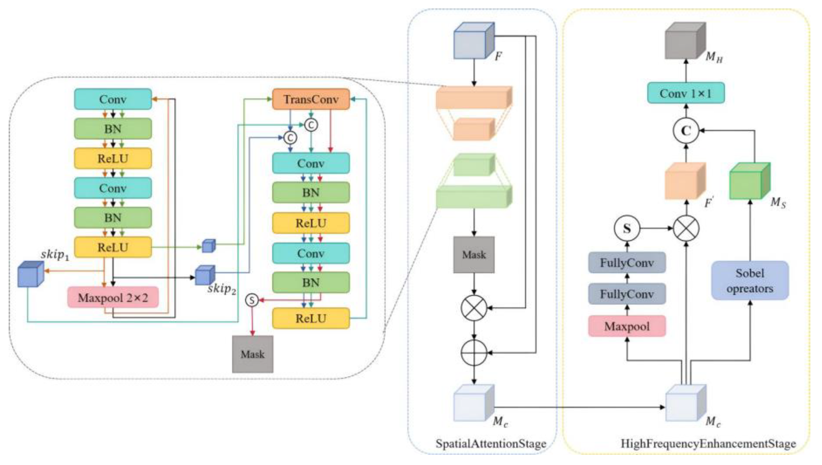
The HFAM follows the design pattern of the convolutional block attention module (CBAM) [18], consisting of two sub-modules: the spatial attention module and the high-frequency enhancement module. Its workflow is illustrated in Figure 2. First, the input feature map $\mathrm{F}$ passes through the spatial attention module, generating a spatial attention mask. The input feature map is then element-wise multiplied with the mask, and the result is summed to produce the spatial attention feature map ${\mathrm{M}}_{\mathrm{c}}$. Subsequently, the spatial attention feature map ${\mathrm{M}}_{\mathrm{c}}$ is passed into the high-frequency enhancement module, where high-frequency features ${\mathrm{M}}_{\mathrm{s}}$ are extracted using the Sobel operator [19]. Meanwhile, a weight map is generated through convolution, and an intermediate feature map ${\mathrm{F}}^{\prime }$ is obtained by element-wise multiplication with the spatial attention feature map. Finally, the intermediate ${\mathrm{F}}^{\prime }$ and high-frequency ${\mathrm{M}}_{\mathrm{s}}$ feature maps are fused along the channel dimension, and the feature map size is adjusted through $1\times 1$ convolution to output the edge features ${\mathrm{M}}_{\mathrm{H}}$.

Specifically, the input feature map first enters a spatial attention module, undergoing a series of convolution operations with batch normalization and ReLU activation applied after each convolution in order to extract the preliminary features. Next, the feature map is gradually reduced in spatial resolution by maximum pooling to extract features at different scales. During this process, the input feature maps are passed through skip connections twice to transmit the original features to subsequent stages for feature fusion. Subsequently, the feature map is gradually restored to the original resolution via two transposed convolution operations and concatenated with the skip-connected features to further enhance multi-scale feature fusion. Next, an attention mask is generated using convolution and a Sigmoid function, which performs element-wise multiplication with the input feature map to highlight salient regions. Finally, the original input feature map is summed with the weighted features to produce the spatial attention map. This is mathematically represented as:

$$Mask=F\odot$$

(1)

$$M_c=F\oplus \left(F\otimes Mask\right)$$

(2)

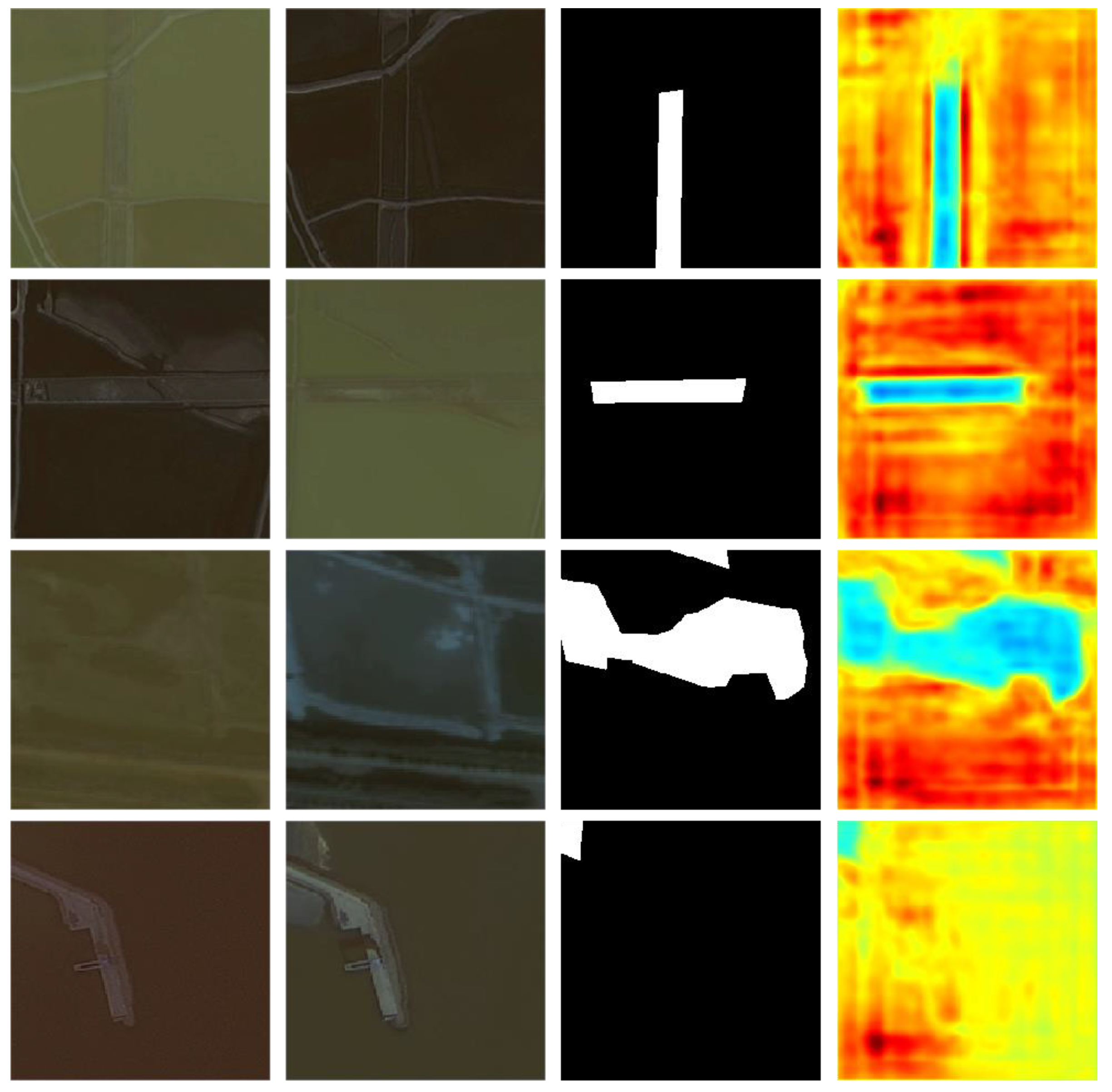
where $\odot$ denotes convolution operation, $\oplus$ denotes element-by-element addition, and $\otimes$ denotes element-by-element multiplication. Figure 3 shows examples of our self-constructed coastal zone change detection dataset and the corresponding edge feature maps obtained after HFAM processing. The edge feature map examples are presented in the form of heatmaps, highlighting the areas of the feature map that the model focuses on during the edge feature extraction stage.

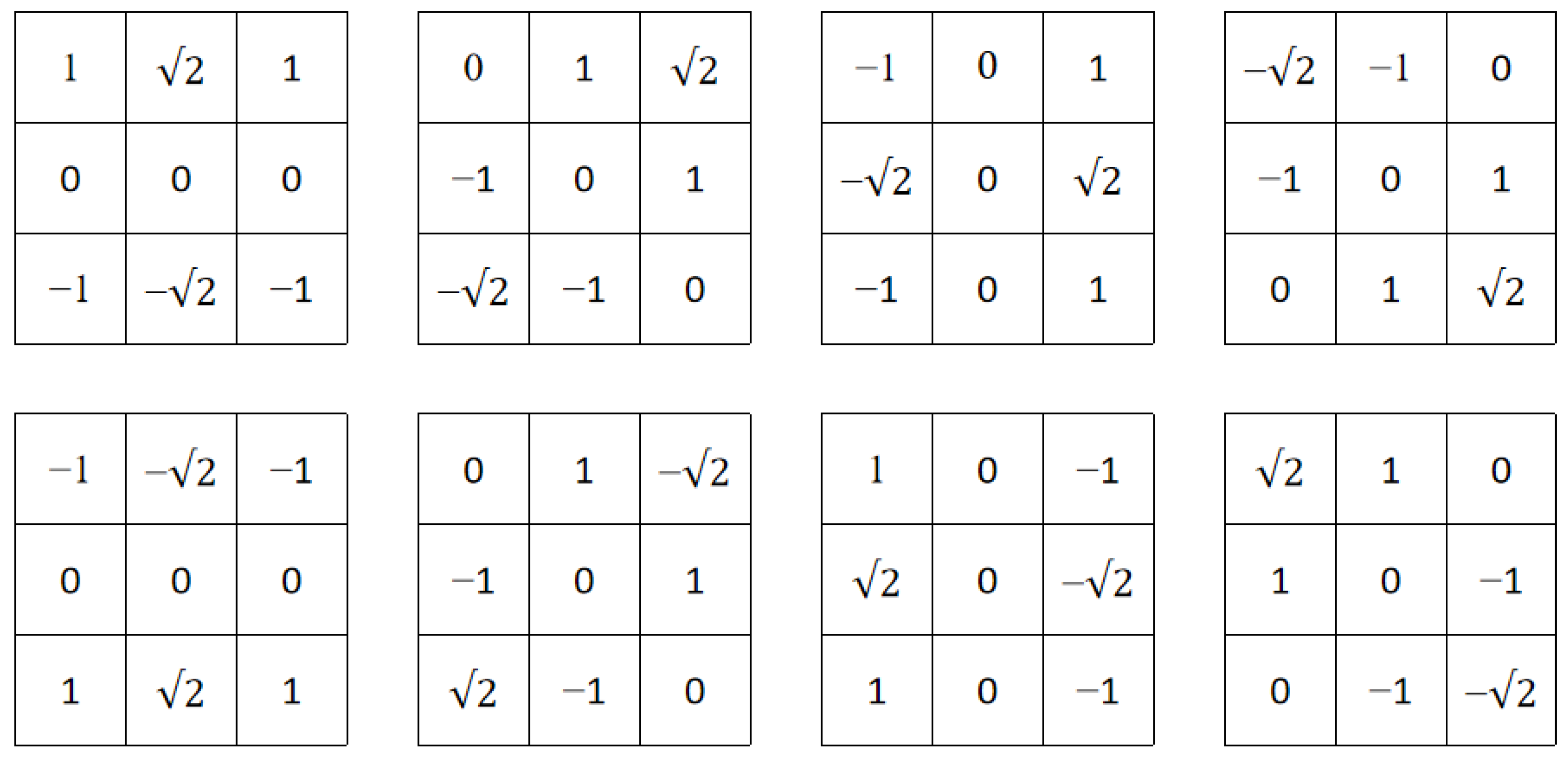
For the high-frequency enhancement module, high-frequency information is initially extracted from the spatial attention map $M_c$ using the Sobel operator to obtain a high-frequency feature map $M_s$. Considering the diversity of the shapes of the changing regions in the coastal zone, we adopt eight Sobel operators with different orientations, as shown in Figure 4. This approach captures edge features more effectively and extracts rich high-frequency information, thus enhancing the model’s ability to recognize changing regions with diverse shapes. In addition, the multi-directional edge features enhance the robustness of the model, effectively suppressing noise and improving the accuracy of change detection.

Secondly, the spatial attention map $M_c$ is first subjected to global maximum pooling, and the pooling result is passed through two fully convolutional layers followed by a Sigmoid activation function. The result is then multiplied element-wise with the spatial attention map $M_c$ to obtain the intermediate feature maps $F^{\prime }$. Next, the high-frequency feature maps $M_s$ are fused with the intermediate feature maps $F^{\prime }$ along the channel axis. Finally, the feature maps are resized to match the input size via $1\times 1$ convolution to produce the output feature maps $M_H$. This is mathematically represented by the following formula:

$$F^{\prime }=M_c\otimes \sigma \left(\odot \left(\odot \left(\mathrm{Maxpool}\left(M_c\right)\right)\right)\right)$$

(3)

$$M_s=\mathrm{Sobel}\left(M_c\right)$$

(4)

$$M_H=\odot \left(F^{\prime }⊚M_s\right)$$

(5)

where $\mathsf{\sigma }$ denotes the Sigmoid function [20], Maxpool denotes maximum pooling, and Sobel denotes the Sobel operator, which $⊚$ denotes the connection along the channel.

By combining spatial attention and high-frequency enhancement, the HFAM effectively captures the edge changes in complex scenes, particularly excelling at handling scenes with irregular boundaries. This approach not only improves the model’s ability to detect fine-grained changes but also strengthens the global representation of the feature map, reducing interference from irrelevant background regions and thereby improving the overall detection performance.

3.2. Contextual Information Integration

In the field of change detection, with the increasing spatial and temporal resolution of remote sensing images, the changing characteristics of complex terrain areas, such as coastal zones, exhibit multi-scale and multi-level properties. Coastal zone change detection often involves various types of changes at different scales, including ocean, land, vegetation, and man-made structures, with these changes being highly heterogeneous in both space and time. For example, coastal erosion, sea-level rise, and anthropogenic development activities can lead to topographic and geomorphological changes at different scales, resulting in both local and global variations in change across the coastal zone. These changes exhibit multi-scale characteristics in space and may also follow multi-stage, variable-frequency patterns over time. Therefore, effectively extracting and integrating change information across different scales and levels is crucial for improving the accuracy of coastal zone change detection.

Although the high-frequency attention module can enhance the model’s ability to capture edge information, this information is often scattered across feature maps at various scales, and effectively integrating it remains a challenge for improving detection accuracy. Therefore, by integrating features from different scales, a richer feature representation is provided to the model, helping it to better identify and capture change areas at different scales in the coastal zone, especially in complex geographic environments, offering a significant advantage. To this end, we introduced the spatio-temporal difference attention module (SDAM) to enhance the performance in coastal zone change detection tasks. Additionally, feature fusion of same-branch feature maps was performed prior to inputting them into the SDAM module. For complex coastal zone areas, changes often exist at multiple scales, and by fusing high-frequency features at various scales, the model’s ability to perceive multi-scale changes is enhanced, making it more adaptable to complex terrain and diverse change types.

3.2.1. Feature Fusion

There are significant differences in spatial resolution and the receptive field between multi-scale features, and feeding them directly into the SDAM module could introduce redundancy and increase the model’s computational burden [21]. Therefore, we resized the feature maps from three different scales of the same branch to a common scale and then fused them element-wise. This effectively integrates information from different scales, reducing redundancy and allowing subsequent modules to process the features more efficiently and focus on extracting useful information. By resizing the feature maps to the same scale, the fused feature map removes scale differences, enabling unified processing of input features in subsequent modules. This helps capture changing area information more accurately.

In addition, changes in coastal zones typically manifest as features of various types and scales, such as localized geomorphological changes and global land-use patterns. High-scale features capture global semantic information, while low-scale features retain rich local details. Feature fusion improves both global and local semantic representations of the model, and element-wise fusion preserves the benefits of all scales in the feature map [22]. This gives a distinct advantage when dealing with diverse changes in the coastal zone.

3.2.2. Spatio-Temporal Difference Attention Module

In change detection tasks, many methods are available for processing the dual-branch feature maps of Siamese networks, including direct subtraction, summation, splicing, and enhancement mechanisms. However, each method has its inherent limitations. The subtraction-based method typically generates a difference map by computing the pixel-wise difference between two temporal images. This approach is simple and intuitive but tends to introduce significant noise under varying lighting conditions, observation angles, and noise disturbances, resulting in error accumulation. The splicing-based method retains the complete information of each temporal phase by concatenating the dual-temporal images along the channel dimension. While this approach preserves more feature information, its main limitation is that it does not provide an explicit representation of change features, and the model must learn to autonomously extract change-related information from the spliced features, making the model’s training highly dependent on the quality and size of the labeled dataset. Therefore, the spatio-temporal difference attention module adopts a two-branch structure consisting of a subtraction branch and a concatenation branch, as shown in Figure 5, aiming to learn both global change-related information at the target level and fine-grained local contexts between the two temporal-phase feature maps.

The subtraction branch computes the absolute difference between the dual-branch feature maps at the same scale, which is then fed into the subsequent coordinate attention module (CAM) to capture the spatio-temporal differences between the dual-temporal feature maps. Since the input dual-temporal images are not ordered temporally, using the absolute difference eliminates the effect of change direction, improves detection symmetry and robustness, reduces interference from negative noise, and unifies the scale of the change features, thereby improving the accuracy and stability of the change detection task. The connection branch concatenates the dual-branch feature maps at the same scale along the channel dimension and then passes through two convolutional layers to extract local context information, thereby supplementing the features and reducing noise interference. The entire process of the SDAM is represented by the following formula:

$$F_D=\left|F_1^{i\left(2\right)}-F_2^{i\left(2\right)}\right|$$

(6)

$$F^{″}=\mathrm{CA}\left(F_D\right)$$

(7)

$$F_C={\odot }_1\left({\odot }_3\left(F_1^{i\left(2\right)}⊚F_2^{i\left(2\right)}\right)\right)$$

(8)

$$F_S=F_C\oplus F^{″}$$

(9)

where $\left|·\right|$ represents the absolute value, CA denotes the coordinate attention module, and ${\odot }_1$ and ${\odot }_3$ are the convolution operations of $1\times 1$ and $3\times 3$, respectively, followed by batch normalization and ReLU activation.

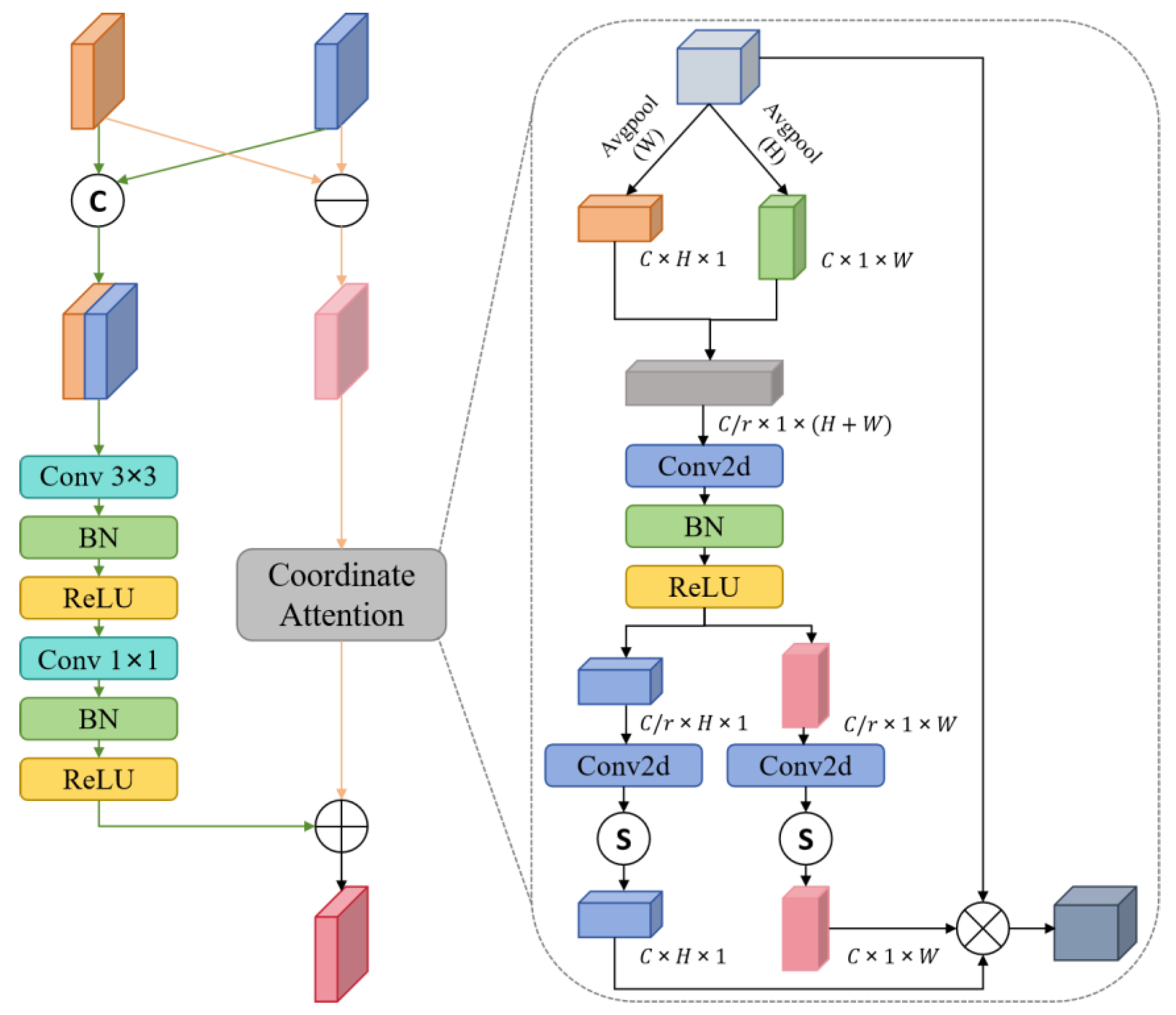
At present, global pooling and convolution operations are widely used in attention mechanisms in both domestic and international change detection research. However, pooling operations compress the feature map into one dimension, leading to a loss of positional details, while convolution operations have a limited receptive field, which hinders the extraction of long-range dependencies. Therefore, in the subtraction branch, we used the coordinate attention module to extract both global and local features. In the coordinate attention module, two average pooling operations with different spatial ranges are applied to encode each channel horizontally and vertically, respectively. The outputs of the pooling layers are concatenated and passed through a $1\times 1$ convolution operation. The resulting tensor is then split into two independent tensors, generating attention vectors with the same number of channels for the horizontal and vertical coordinates of input X. Finally, the two tensors are multiplied element-wise with the absolute difference feature map $F_D$ to obtain the intermediate feature map $F^{″}$. The formula indicates:

$$F_h=poo{l}^h\left(F_D\right)$$

(10)

$$F_w=poo{l}^w\left(F_D\right)$$

(11)

$$f=\delta \left({\odot }_1\left(\left[F_h,F_w\right]\right)\right)$$

(12)

$$F_h^{\prime },F_w^{\prime }=\mathrm{Split}\left(f\right)$$

(13)

$$F_h^{″}=\sigma \left({\odot }_1^{\mathrm{h}}\left(F_h^{\prime }\right)\right)$$

(14)

$$F_w^{″}=\sigma \left({\odot }_1^{\mathrm{w}}\left(F_w^{\prime }\right)\right)$$

(15)

$$F^{″}=F_D\otimes \left(F_h^{″}\times F_w^{″}\right)$$

(16)

where $poo{l}^h$ and $poo{l}^w$ denote the average pooling in vertical and horizontal coordinates, respectively, $\delta$ denotes the ReLU function, $\sigma$ denotes the Sigmoid function, and $\times$ denotes matrix multiplication.

The connected branch consists of a $3\times 3$ convolutional block for learning local information in the input feature map and a second $1\times 1$ convolutional block to reduce the number of channels in the feature map, ensuring that the output matches the output features of the subtraction branch. This design not only helps capture small-scale variations and subtle features but also simplifies feature fusion by ensuring consistency in the feature dimensions between the two branches. Each convolution block consists of convolution operations, batch normalization, and ReLU activation, which improves feature processing efficiency and enhances the model’s stability.

In addition, feature extraction and channel tuning in the connected branch reduce the model’s dependence on a specific change detection dataset. In change detection tasks, where datasets often differ and phase subtraction operations may introduce inconsistency or noise, the connected branch further optimizes features through an effective convolutional structure, thus improving the model’s generalization ability across different datasets. This design enables the connected branch to provide richer, more stable feature representations when paired with the subtraction branch, which allows the model to detect changes more accurately while reducing overfitting to specific datasets.

Figure 6 shows examples of the coastal zone change detection dataset and the corresponding intermediate feature maps obtained after SDAM processing. The intermediate feature map examples are presented in the form of heatmaps, highlighting the areas of the feature map that the model focuses on during the Contextual Information Integration stage. Compared to Figure 3, it is evident that the model pays more attention to the change areas with higher precision, and false positives and missed detections are significantly reduced.

3.3. Change Result Generation

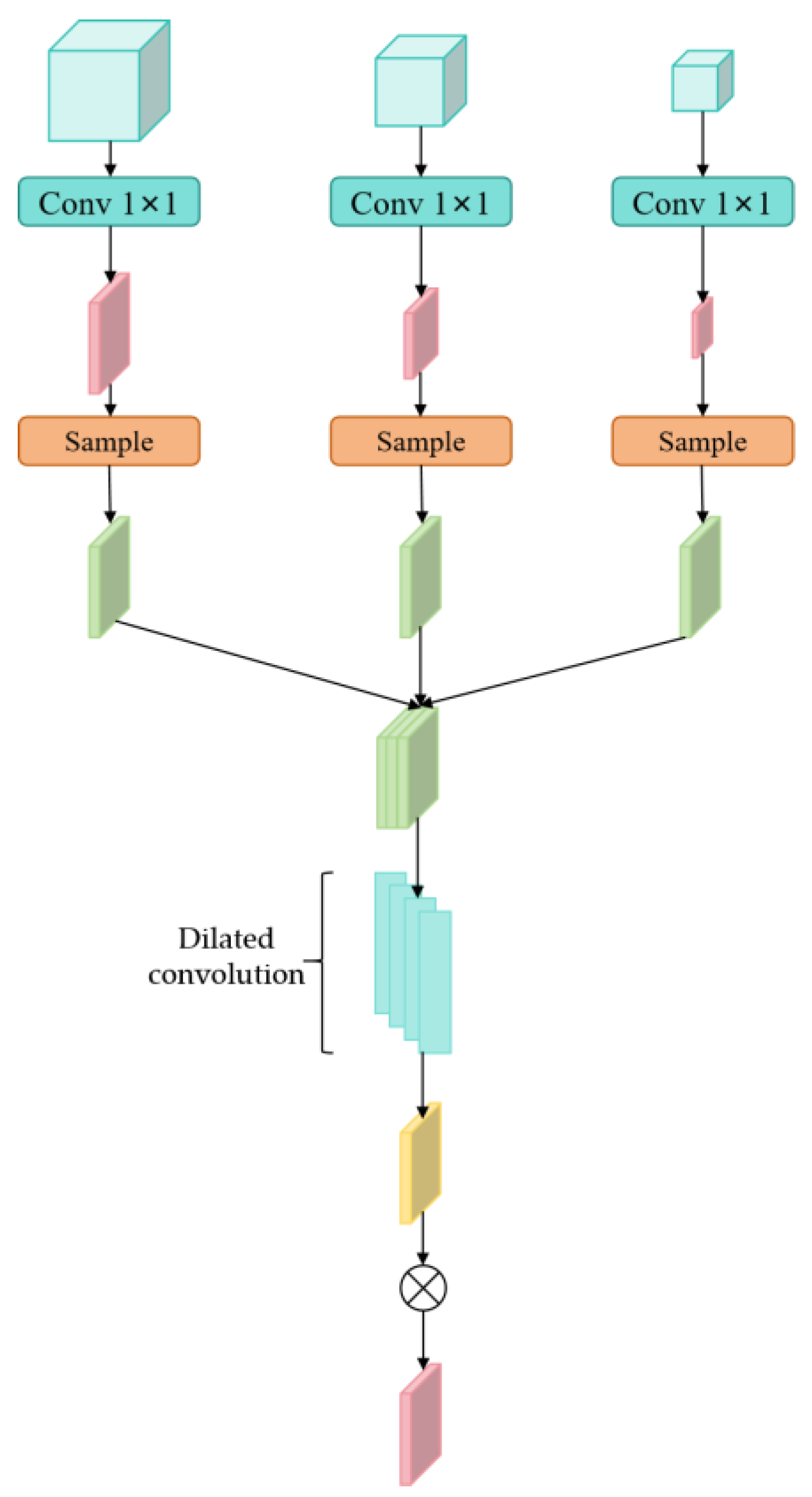
As shown in Figure 7, this paper inputs the three feature maps $F^{i\left(4\right)}\left(\forall i\in \left\{1,2,3\right\}\right)$, integrated by the spatio-temporal difference attention module into the foreground attention module to obtain the foreground feature map $F^{\left(5\right)}$. They are then passed into the classifier to produce the change result map $P$.

We simulated the human eye’s observation mechanism, where attention gradually shifts from the background to the foreground, and designed the foreground attention module to enhance coastal zone change detection accuracy by integrating multi-scale feature maps, thereby mitigating the effects of class imbalance. In change detection, the foreground typically represents the changed region, while the background corresponds to the unchanged or irrelevant areas. The foreground attention module integrates features from different scales based on multi-scale feature extraction, allowing the model to explore the relationship between changing and unchanged regions during training, thereby improving the learning of change information.

The structure of the foreground attention module is shown in Figure 7. We first aligned the feature maps at different scales by applying a $1\times 1$ convolutional layer to adjust their channel sizes. Next, the feature maps were resized to the same size through a sampling operation. The feature maps were then concatenated along the channel dimension to form a fine feature map $F_a$. The fine feature was then passed through four consecutive dilated convolution layers, with the output channels set to [512, 512, 512, 256] to further integrate the contextual information with a larger receptive field. Finally, the output of the dilated convolution layers was multiplied element-wise with the original fine feature map to obtain the final foreground feature map $F^{\left(5\right)}$, as denoted by Equations (17) and (18).

$$F_a={\mathrm{C}}_{\mathrm{𝒾}=1}^3\left(\mathrm{Samp}\left(\odot \left(F^{i\left(4\right)}\right)\right)\right)$$

(17)

$$F^{\left(5\right)}=F_a\otimes \left(F_a\odot {\mathrm{D}}_1\left(r\right)\odot {\mathrm{D}}_2\left(r\right)\odot {\mathrm{D}}_3\left(r\right)\odot {\mathrm{D}}_4\left(r\right)\right)$$

(18)

where Samp refers to the sampling operation, $\mathrm{C}\left(·\right)$ refers to concatenating the three feature maps along the channel dimension, and ${\mathrm{D}}_{\mathrm{k}}\left(r\right)$ refers to a series of dilated convolution layers with a dilation rate, r (dilation rate of 3, 4 layers).

In this model, the coastal zone change detection network can better correlate the contextual information related to the changes and focus more on the changed regions, effectively mitigating the imbalance problem. Figure 8 shows examples of the coastal zone change detection dataset and the corresponding foreground feature maps obtained after FAM processing. The foreground feature map examples are presented in the form of heatmaps, highlighting the areas of the feature map that the model focuses on during the multi-scale feature map integration stage. Compared to Figure 3 and Figure 6, it is evident that the model pays more attention to the change areas with higher precision, and false positives and missed detections are significantly reduced. However, to further improve the model’s detection ability, the design of the loss function is crucial. An effective loss function can optimize the model training process and reduce the impact of random errors on the model. Therefore, we have optimized the loss function design.

Optimal Design of the Loss Function

The output feature map $F^{\left(5\right)}$ is passed to the classifier to produce three change result maps, $P_1$, $P_2$, and $P_3$. The focal loss and dice loss for each change result map are calculated separately. The sum of these two loss values gives the loss for each change result map, and the total loss for the change detection task is the sum of the losses for the three change result maps.

Let $\mathrm{Y}$ be the true value, $p_t$ the model’s predicted probability for the correct category, $L_{fl}$ the focal loss, $L_{dl}$ the dice loss, and $L_{total}$ the total loss. The overall loss function for the coastal zone change detection task is as follows:

$$L_{fl}\left(P_i,\mathrm{Y}\right)=-{\left(1-p_t\right)}^{\gamma }\log \left(p_t\right)$$

(19)

$$L_{dl}\left(P_i,\mathrm{Y}\right)=1-{\displaystyle \frac{\left|P_i\cap \mathrm{Y}\right|}{\left|P_i\right|+\left|\mathrm{Y}\right|}}$$

(20)

$$L_{total}={\sum }_{\mathrm{i}=1}^3\left(L_{fl}\left(P_i,\mathrm{Y}\right)+L_{dl}\left(P_i,\mathrm{Y}\right)\right)$$

(21)

where $\gamma$ is the adjustment factor for focal loss, used to adjust the model’s focus on change samples (set to 0.5 in our case).

Focal loss dynamically reduces the contribution of easily classified samples by introducing an adjustment factor. For easily classified non-change samples, $p_t$ is close to 1, making ${\left(1-p_t\right)}^{\gamma }$ close to 0 and reducing their loss weights. Similarly, for hard-to-classify change samples, $p_t$ is smaller than for the non-change samples, making ${\left(1-p_t\right)}^{\gamma }$ larger, which increases the loss weight for the change samples. Dice loss, on the other hand, measures the similarity by calculating the proportion of overlap between the predicted results and true labels, which is nearly unaffected by class imbalance. In fact, dice loss effectively measures the performance of minority classes through the overlap ratio.

4. Experiment

4.1. Evaluation Indicators

According to the widely used evaluation schemes in change detection research, the following evaluation metrics are used in this paper: Intersection over Union (IoU), precision, recall, F1 score, overall accuracy (OA), and the Kappa coefficient. IoU is commonly used to measure the overlap between the detected change region and the true change region, and it is the primary reference metric in this paper. Precision refers to the proportion of the detected change region that is correctly identified as changed. Recall indicates the proportion of the actual change regions successfully detected by the algorithm. The F1 score combines precision and recall, and a high F1 score indicates a good balance between precision and recall, considering both the accuracy and completeness of the detected change regions.

Overall accuracy (OA) represents the proportion of correctly classified samples in a change detection task, i.e., the ratio of the total number of correctly classified samples to the total number of samples. The Kappa coefficient measures the consistency between the algorithm’s detection results and the ground truth.

All the above metrics are based on confusion matrices, which help analyze classifier performance by showing the relationship between the actual and predicted categories. The confusion matrix typically contains the following four key metrics:

• True Positives (TP): the number of samples where the actual change class is correctly predicted as the change class;
• True Negatives (TN): the number of samples where the actual non-change class is correctly predicted as the non-change class;
• False Positives (FP): the number of samples where the actual non-change class is incorrectly predicted as the change class;
• False Negatives (FN): the number of samples where the actual change class is incorrectly predicted as the non-change class.

The structure of the confusion matrix is illustrated in

Table 1. Confusion matrix.

	Predicted Change Class (Change)	Predicted Change Class (No Change)
Actual Change Class	TP	FN
Actual No Change Class	FP	TN

.

The formulae for these evaluation indicators are shown below:

$$\mathrm{IoU}={\displaystyle \frac{\mathrm{TP}}{\mathrm{TP}+\mathrm{FP}+\mathrm{FN}}}$$

(22)

$$\mathrm{Pr}={\displaystyle \frac{\mathrm{TP}}{\mathrm{TP}+\mathrm{FP}}}$$

(23)

$$\mathrm{Rc}={\displaystyle \frac{\mathrm{TP}}{\mathrm{TP}+\mathrm{FN}}}$$

(24)

$$\mathrm{F}1={\displaystyle \frac{2\times \mathrm{Pr}\times \mathrm{Rc}}{\mathrm{Pr}+\mathrm{Rc}}}$$

(25)

$$\mathrm{OA}={\displaystyle \frac{\mathrm{TP}+\mathrm{TN}}{\mathrm{TP}+\mathrm{TN}+\mathrm{FP}+\mathrm{FN}}}$$

(26)

$$\mathrm{Kappa}={\displaystyle \frac{{\mathrm{P}}_{\mathrm{o}}-{\mathrm{P}}_{\mathrm{e}}}{1-{\mathrm{P}}_{\mathrm{e}}}}$$

(27)

where $P_o$ denotes the case in which the model prediction and the actual are in agreement, i.e., the OA. $P_e$ refers to the probability that the predicted outcome will be in agreement with the actual case, assuming random guessing, calculated as follows:

$$P_e=\left({\displaystyle \frac{\left(TP+FP\right)\times \left(TP+FN\right)}{N^2}}\right)+\left({\displaystyle \frac{\left(FN+TN\right)\times \left(FP+TN\right)}{N^2}}\right)$$

(28)

where $N$ denotes the total number of samples, calculated as:

$$\mathrm{N}=\mathrm{TP}+\mathrm{FP}+\mathrm{TN}+\mathrm{FN}$$

(29)

4.2. Experimental Data

4.2.1. Public Dataset

In order to validate the effectiveness of AMMNet, the public dataset LEVIR_CD used in the literature [4,5,6,7,8] is selected for validation and comparison.

The LEVIR-CD dataset is recognized as a key benchmark in remote sensing, specifically designed for building change detection. It consists of 637 pairs of high-resolution remote sensing images, each with a 0.5 m/pixel resolution, covering building changes in urban China from 2002 to 2017. To meet the model and GPU memory constraints, each sample is cropped into 16 non-overlapping image patches and split into training, validation, and test sets with a 7:1:2 ratio, containing 7120, 1024, and 2048 image pairs, respectively. The dataset covers a variety of urban development scenarios and complex environments, providing rich and diverse data to support model performance validation.

4.2.2. Coastal Zone Change Detection Dataset (BCZ_CD)

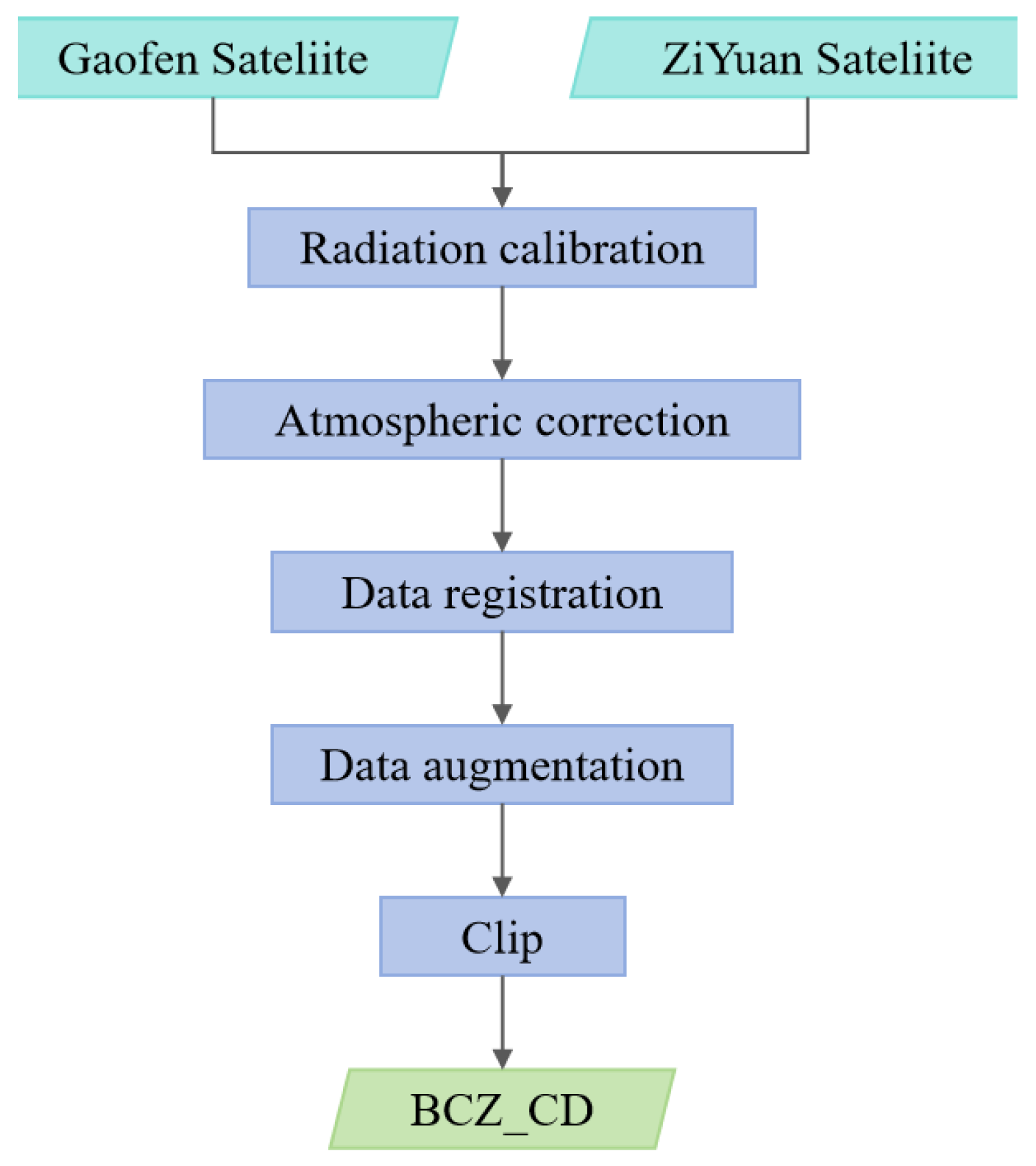
We acquired multi-temporal remote sensing data from September to December for the coastal zones of Tianjin, Liaoning, Shandong, and Hebei provinces using Gaofen series satellites (GF1, GF1B, GF1C, GF1D, GF2, GF6) and resource series satellites (ZY302, ZY1E). The selected provinces cover diverse natural environments, ranging from estuarine wetlands to sandy coasts, coastal plains, and mudflat saline–alkaline lands, and have been significantly impacted by human activities such as reclamation, port construction, marine aquaculture, and industrial expansion. This ensures the dataset’s representativeness in both spatial and ecological diversity. The image data, which were collected during the autumn and winter seasons, capture seasonal features such as vegetation withering, tidal changes, and shoreline morphology adjustments, reflecting the complex dynamics of the coastal zone under the combined effects of climate change and human activities.

Based on expert-provided change patch data, the images were divided into 77 pairs of pre- and post-change remote sensing images. The images underwent ortho-correction, radiometric calibration, atmospheric correction, and resampling, resulting in 128 cropped pairs of images. These preprocessing steps eliminate geometric and radiometric errors, improve image contrast and consistency, and provide a high-quality dataset for subsequent change detection.

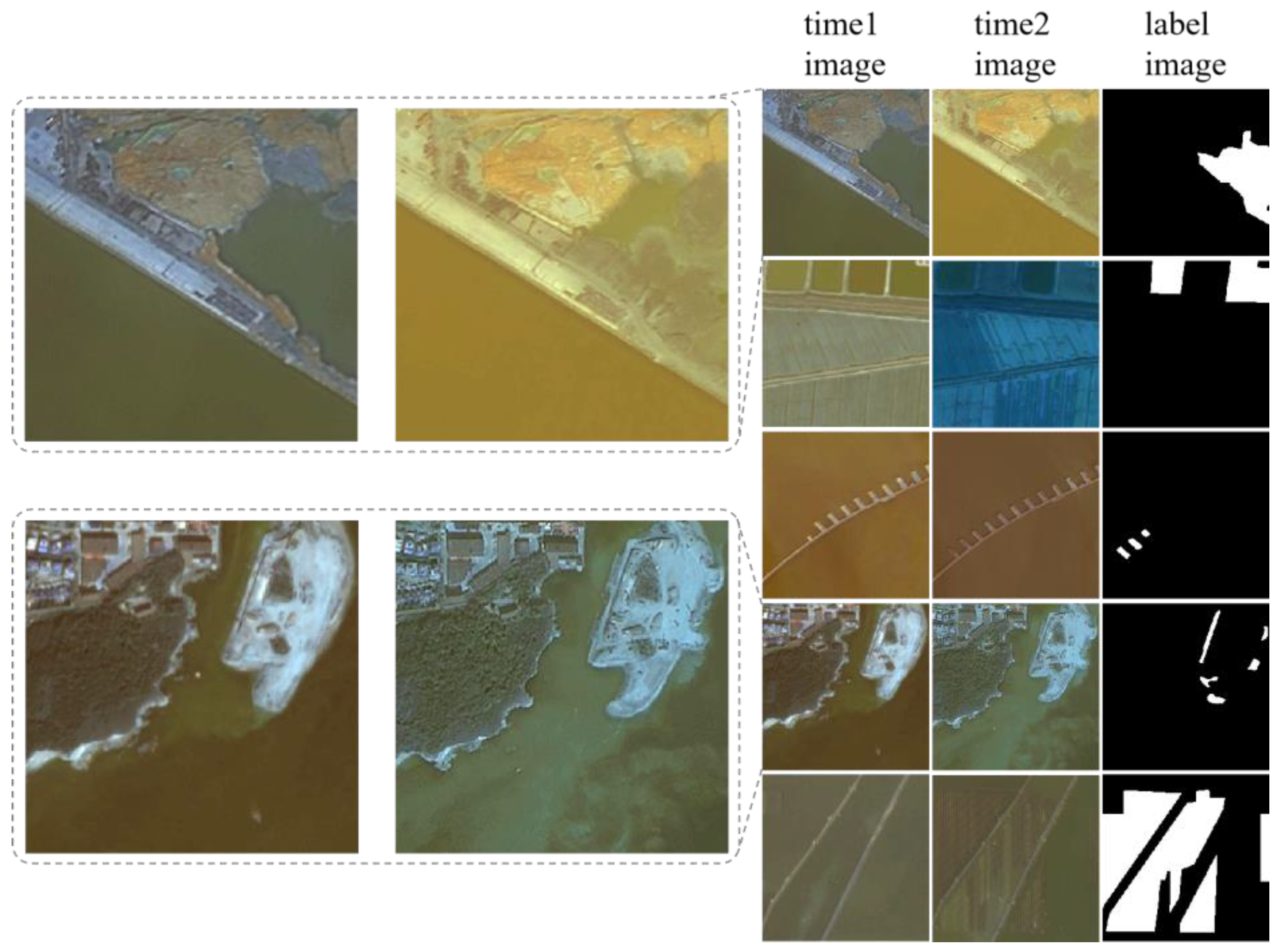
To meet the model’s data volume requirements and GPU memory limitations, the dataset was augmented through rotation and flipping. Each image was then cropped into 16 non-overlapping patches, as shown in Figure 9. This data augmentation method not only expands the dataset but also increases its diversity, enabling the model to better adapt to different change patterns and noise interference, thus enhancing its generalization ability. Ultimately, 6048 sample pairs were created and split into training and test sets (5536/512). The coastal zone change detection dataset (BCZ_CD) is shown in Figure 10.

4.3. Comparative Experiments

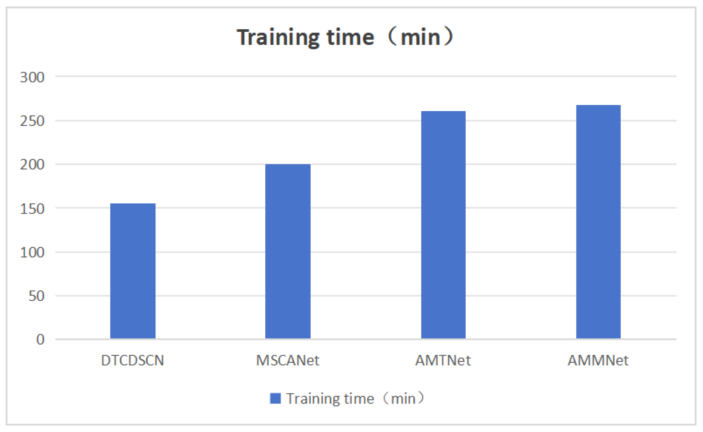
We implemented the coastal zone change detection model in PyTorch, using ImageNet-pretrained ResNet as the backbone. The input size was set to 256 pixels for training, and the AdamW optimizer was used for parameter optimization. After adjusting the parameters, the batch size for training and testing was set to 8, the initial learning rate to 0.0001, and the weight decay coefficient to 0.01. The experiments were conducted on an NVIDIA Tesla A100 SXM2 40GB, with each experiment trained for 150 epochs. Validation was performed after each epoch, and the best model was selected for evaluation on the test set.

To demonstrate the effectiveness of our model, we compared it with several leading change detection models from the past five years, using both our self-built coastal zone change detection dataset and the public LEVIR_CD dataset. Our model incorporates a high-frequency attention module, a spatio-temporal difference attention module, and a foreground attention module, all based on a multi-scale Siamese network while also optimizing the loss function. After 150 iterations, the model accuracy was obtained, as shown in

Table 2. Comparison of the results with other state-of-the-art change detection methods on BCZ_CD.

Method	BCZ_CD
	IoU	Pre.	Rec.	F1	OA	Kappa
DTCDSCN	73.123	91.065	78.775	84.475	97.556	83.157
MSCANet	73.800	82.130	87.090	83.330	99.570	84.470
AMTNet	83.818	88.877	93.641	91.197	99.496	90.938
AMMNet	90.263	94.605	95.161	94.882	99.714	94.735

Blue represents the highest accuracy under this evaluation metric.

and

Table 3. Comparison of the results with other state-of-the-art change detection methods on LEVIR_CD.

Method	LEVIR_CD
	IoU	Pre.	Rec.	F1
DTCDSCN	78.050	88.530	86.830	87.670
MSCANet	81.660	91.300	88.560	89.910
AMTNet	83.080	91.820	89.710	90.760
AMMNet	83.662	92.208	90.026	91.104

Blue represents the highest accuracy under this evaluation metric.

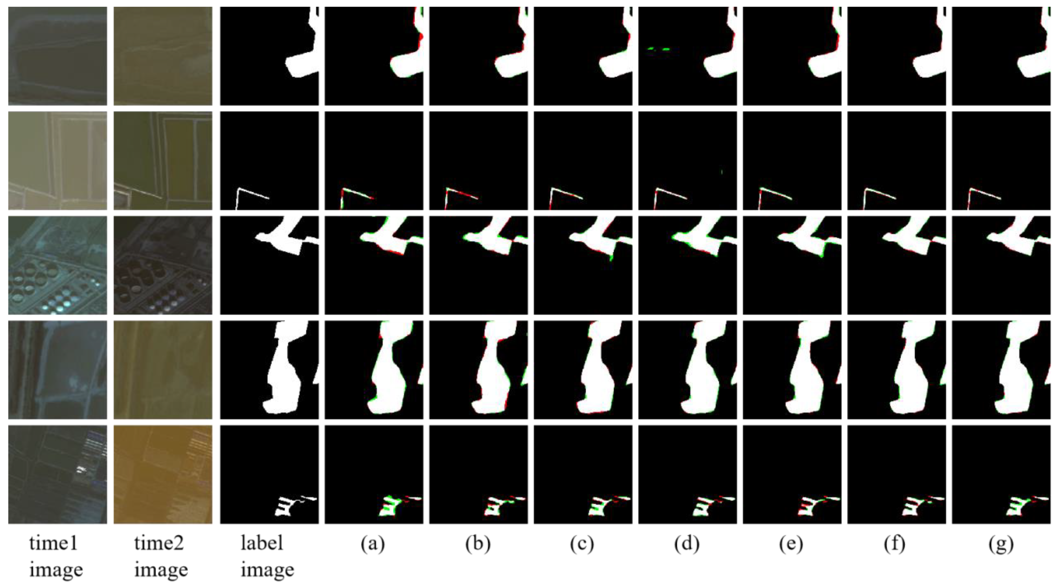
. Figure 11 present a comparison of accuracy for the different methods on the coastal zone change detection dataset (BCZ_CD) in the form of line charts. Figure 12 shows a typical example of the detection results for different methods on the coastal zone change detection dataset. Figure 13 presents a comparison of accuracy for the different methods on the public change detection dataset (LEVIR_CD) in the form of a line chart.

Table 2 and Table 3 compare the performance of the AMMNet model with several existing change detection models, including DTCDSCN, MSCANet, and AMTNet, on two datasets. First, on BCZ_CD, as shown in Table 2, the AMMNet model performs well across all metrics, particularly in IoU (90.263%), precision (94.605%), and recall (95.161%). The F1 score reaches 94.882%, indicating high accuracy in coastal zone change detection. AMMNet leads in the IoU metric, indicating greater accuracy in capturing actual change areas, better identifying true changes, and minimizing false alarms. High scores in precision and recall show that AMMNet achieves an optimal balance between the two, ensuring accurate predictions while minimizing false negatives. The F1 score further confirms AMMNet’s superiority in overall detection capability, reflecting its ability to handle complex change scenarios. These results show that AMMNet performs well in specific scenarios and demonstrates broad adaptability for other change detection tasks.

Secondly, as shown in Table 3 and Figure 13, the AMMNet model performs well on the LEVIR_CD dataset, remaining leading in key metrics such as the IoU, precision (Pr), recall (Rc), and F1, with the F1 score, reaching 91.104%. This further proves AMMNet’s adaptability and robustness across various scenarios. The LEVIR_CD dataset is widely used as a benchmark for evaluating model performance in complex scenarios due to its diversity and extensive usage. AMMNet maintains high Pr and Rc values, demonstrating strong detection capabilities and accuracy across different scenarios, suggesting that AMMNet has strong generalization ability.

4.4. Ablation Experiment

To assess the importance of the global and foreground attention modules, ablation experiments were designed with seven configurations: without the HFAM, SDAM, or FAM; HFAM only; SDAM only; FAM only; and combinations of two modules. Model accuracies for each configuration are shown in

Table 4. Comparison of the results under the ablation experiment.

Method	HFAM	SDAM	FAM	IoU	Pre.	Rec.	F1	OA	Kappa
AMMNet	√	×	×	81.411	85.852	94.026	89.753	99.402	89.446
AMMNet	×	√	×	84.328	90.815	92.191	91.498	99.523	91.252
AMMNet	×	×	√	88.239	92.850	94.672	93.752	99.648	93.571
AMMNet	√	√	×	88.213	91.936	95.611	93.737	99.644	93.554
AMMNet	√	×	√	89.328	94.944	93.789	94.363	99.688	94.203
AMMNet	×	√	√	90.008	94.126	95.349	94.741	99.705	94.589
AMMNet	√	√	√	90.263	94.605	95.161	94.882	99.714	94.735

× indicates that the corresponding configuration of the attention module is disabled in the ablation experiment, while √ indicates that it is not disabled. Blue represents the highest accuracy under this evaluation metric.

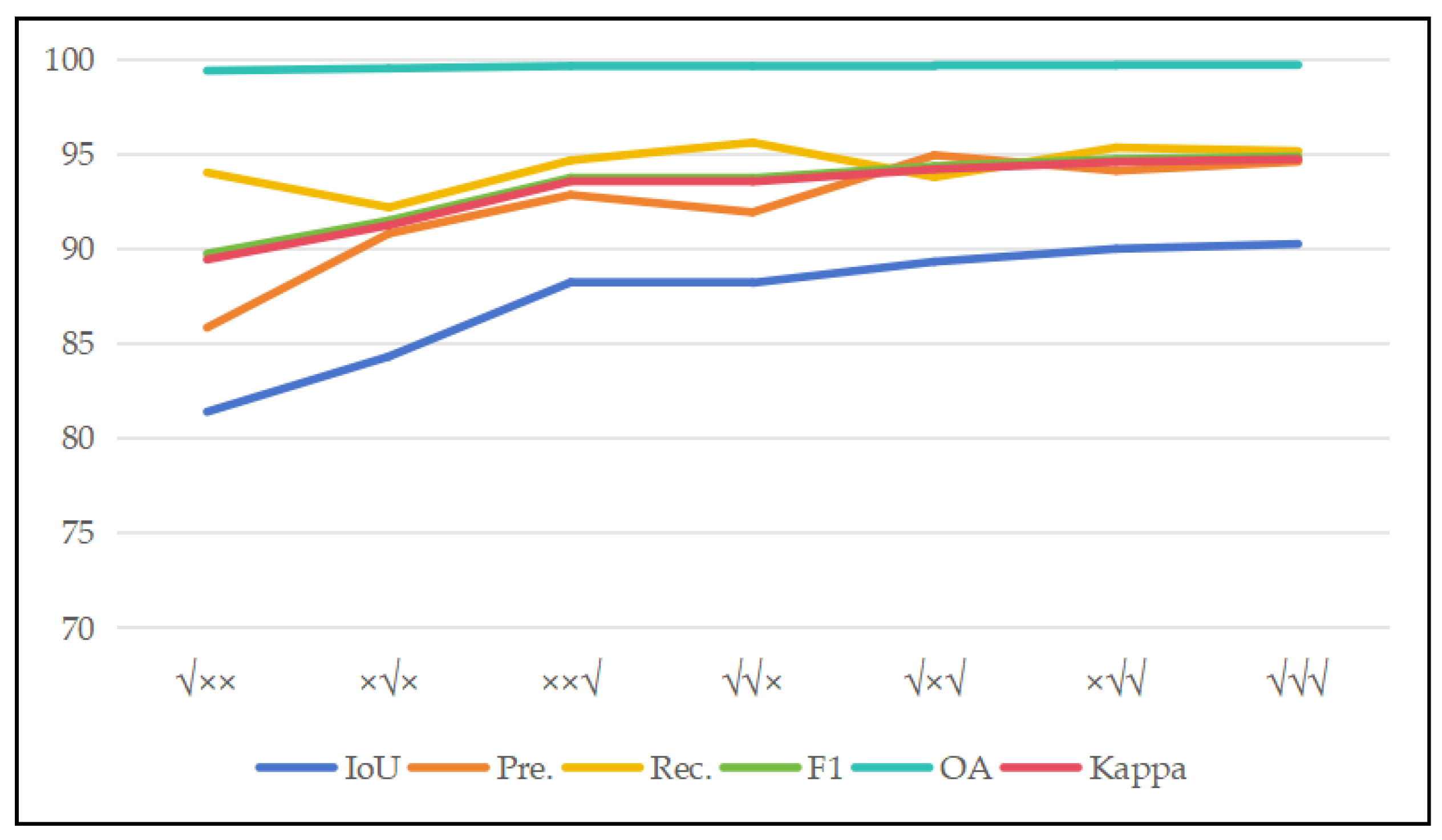
. Figure 14 visually presents a comparison of accuracy for different configurations in the ablation experiment on the coastal zone change detection dataset (BCZ_CD) in the form of a line chart. The sample results for each configuration are shown in Figure 15.

In the initial experiments, using only the HFAM, the model achieved an IoU of 81.411%, indicating that it could capture key features but still showed limitations in fine-grained change detection. With the SDAM, performance improved, with an IoU of 84.328%, precision of 90.815%, recall of 92.191%, and an F1 score of 91.498%. This suggests that the SDAM helps the model balance precision and comprehensiveness, particularly improving recall and the F1 score, allowing for better identification of the change regions and reducing detection leakage.

Adding the FAM improved the IoU to 88.239%, with the precision and recall at 92.850% and 94.672%, and the F1 score at 93.752%. This improvement highlights the FAM’s role in enhancing accurate segmentation and the model’s ability to localize change regions more precisely.

Further results showed that when both the HFAM and SDAM were used, performance reached new heights: the IoU was 88.213%, precision was 91.936%, the recall was 95.611%, and the F1 score was 93.737%. This combination demonstrates that the HFAM and SDAM complement each other, enhancing both accuracy and the model’s comprehensive perception of the change regions.

When all three modules—the HFAM, SDAM, and FAM—are used together, the model’s performance reaches its optimal state: the IoU is 90.263%, precision is 94.605%, the recall is 95.161%, the F1 score is 94.882%, OA is 99.714%, and the Kappa is 94.735%. This configuration results in high overall accuracy and Kappa while also achieving optimal values in key metrics such as the IoU, precision, recall, and F1 score. The improvement in the F1 score demonstrates the model’s excellent balance between precision and recall, with strong change detection capability and a low false alarm rate.

In summary, the ablation experiments show that combining the HFAM, SDAM, and FAM significantly improves AMMNet’s performance in change detection. Each module positively impacts different performance metrics, particularly the IoU, precision, recall, F1 score, OA, and Kappa, greatly enhancing model accuracy and stability. This suggests that combining different attention mechanisms enhances the model’s fine-grained recognition and robustness in complex scenarios.

5. Conclusions

In this work, we propose AMMNet, a multi-scale coastal zone change detection method that leverages advanced attention mechanisms to address the challenges of feature extraction and class imbalance in coastal zone change detection tasks. The model integrates the high-frequency attention module (HFAM), spatio-temporal difference attention module (SDAM), and foreground attention module (FAM) to enhance feature extraction and contextual integration.

The model first extracts multi-scale features using a ResNet backbone and optimizes them via the HFAM. The fused feature maps are then processed by the SDAM, capturing both global and fine-grained local change information. The FAM further refines these features, allowing the model to focus on change regions, ultimately generating the change map through a thresholding process.

We used remote sensing data from Gaofen and resource series satellites covering Tianjin, Liaoning, Shandong, and Hebei provinces to create the BCZ_CD dataset for training and testing. The experimental results show that AMMNet outperforms the traditional methods across all six key evaluation metrics—the IoU, precision (Pr), recall (Rc), F1 score, overall accuracy (OA), and Kappa. Specifically, AMMNet achieved outstanding results in the IoU (90.263%) and Kappa (94.735%), which demonstrate its superior performance and consistency in coastal zone change detection.

Further validation on the LEVIR_CD public dataset confirms AMMNet’s generalizability and adaptability to different coastal environments. The ablation experiments demonstrated that incorporating the HFAM, SDAM, and FAM significantly enhances model performance, with the best results achieved when all three modules were combined, highlighting the synergy of these attention mechanisms.

In summary, AMMNet combines multi-scale feature extraction with powerful attention mechanisms, leading to substantial improvements in detection accuracy and model generalization. However, the model’s computational complexity and large size remain challenges for real-time deployment on general-purpose hardware. Future work will focus on optimizing the network architecture to reduce these limitations and improve scalability, enabling broader deployment in real-world applications.

6. Limitations and Future Research Directions

6.1. Training Efficiency of the Method

To evaluate AMMNet’s computational efficiency, we compared its training time with that of other change detection models (DTCDSCN, MSCANet, AMTNet). While AMMNet excels in accuracy, its complex network structure results in longer training times. Therefore, comparing the training efficiency of different models is essential for a more comprehensive evaluation of their practical application.

Table 5. Comparison of the training times.

Method	Training Time
DTCDSCN	155 m 21 s
MSCANet	200 m 21 s
AMTNet	260 m 21 s
AMMNet	267 m 21 s

compares the training times of the models under the same experimental conditions. Figure 16 presents a more intuitive comparison of the training times in the form of a bar chart based on the data from Table 5.

Although AMMNet’s training time (267 min and 21 s) is significantly longer than that of other models, this is partly due to its complex structure, which includes the high-frequency attention module (HBAM), spatio-temporal disparity attention module (SBAM), and foreground attention module (FAM), resulting in higher accuracy and better detection performance. Increased model complexity inevitably lengthens the training time, but the additional computational overhead results in significant accuracy improvements, particularly in core metrics such as the IoU, precision (Pre), and recall (Rec).

However, the longer training time remains an area for optimization. Therefore, in future work, we aim to optimize the network structure and reduce computational complexity through a lightweight model design to shorten the training time and enhance scalability in practical applications.

6.2. Single Sobel Operator

While the proposed method effectively constructs the high-frequency attention module (HFAM) using the Sobel operator to enhance feature extraction, it does not consider other operators, such as the Laplacian, Scharr, and Prewitt operators. These alternative operators have distinct characteristics and potential advantages in edge detection and feature extraction. Moreover, comparative experiments between Sobel and these operators were not included in this study. In future research, we plan to incorporate this group of experiments to explore the impact of different operators and their optimized combinations on improving feature extraction performance. This exploration may further optimize the HFAM and enhance the overall accuracy and robustness of the model.