Multicriteria Methodology for Evaluating Energy Management Strategies in Heavy-Duty Fuel Cell Electric Vehicles via Vehicular Models

Abstract

In this paper, a methodology for selecting the Energy Management Strategy (EMS) that best suits a heavy-duty Fuel Cell Electric Vehicle (FCEV) operating under specific conditions along a given driving cycle is proposed. Using a simulation model that incorporates the powertrain architecture and components of a specific FCEV—validated through a more detailed model operating at the power converter switching level—the performance of the entire system can be tested under different EMSs. The multicriteria evaluation system developed in this study enables the calculation of hydrogen and energy consumption, as well as the aging of the battery and fuel cell associated with each EMS. The proposed methodology serves as an evaluation tool for both the dimensioning of powertrain components and the selection of the EMS that best meets the operational requirements of a given FCEV. Results demonstrate that applying this methodology to a use case tailored for commercial devices and a standard driving cycle enables the identification of the most suitable EMS, minimizing hydrogen and energy consumption while reducing battery and fuel cell aging.

1. Introduction

Electric vehicles (EVs) have experienced rapid development in recent decades, driven by economic and environmental concerns surrounding internal combustion engine vehicles. Among the solutions developed, battery electric vehicles (BEVs) have become the most widely adopted, although considerable research has also been dedicated to Fuel Cell Electric Vehicles (FCEVs). Although BEVs appear to be the most cost-effective solution to date, there is significant development around FCEVs, predicting a reduction in hydrogen production costs, particularly for green hydrogen obtained from renewable energy sources. FCEVs offer several advantages compared to BEVs, such as faster refueling times, extended range, and greater suitability for long-range and heavy-duty applications. The main design of an FCEV includes a fuel cell system and a battery pack; however, this configuration faces a well-known drawback: its efficiency remains significantly limited [1].

The efficiency and performance of Fuel Cell Electric Vehicles (FCEVs) largely depend on the implemented Energy Management System (EMS), which optimizes power distribution between the fuel cell and the battery according to various operational criteria. Over the past decade, numerous EMS strategies have been explored in the literature, including rule-based, optimization-based, and learning-based approaches. Selecting the most appropriate EMS is complex; the optimal choice depends on factors such as powertrain configuration, energy storage system (ESS) sizing, driving cycle, and the operational variables that the control system seeks to optimize. Several studies have compared different EMS approaches for FCEVs based on distinct criteria. For instance, in [2], a comparative analysis of energy and exergy efficiency was conducted between fuzzy logic and power-following control strategies across various driving cycles, revealing that fuzzy logic is more efficient for both energy and exergy. In [3], researchers evaluated trainable integrated prediction EMS (TIP-EMS) against predictive strategies over 27 driving cycles, finding that TIP-EMS achieved superior energy conservation and efficiency. Study [4] compared real-time EMS strategies, specifically an Adaptive Equivalent Consumption Minimization Strategy (A-ECMS) and a Stochastic Dynamic Programming (SDP) approach, under random driving cycles, assessing robustness. The results indicated that A-ECMS performs poorly when responding to unknown demand profiles. A complete evaluation of six EMS under realistic driving cycles is performed in [5], but it focuses on the EMS comparison using a simplified vehicle model and only considers fuel cell degradation.

Despite these comparative studies, the authors of this work found no comprehensive methodology for selecting the most suitable EMS tailored to specific powertrain configurations, ESS sizing, and driving cycles. Additionally, although some technical studies consider fuel cell efficiency and aging [6,7,8], few address both fuel cell and battery aging together.

This paper presents a novel methodology for selecting an EMS that minimizes both fuel cell and battery aging while reducing hydrogen and energy consumption in a heavy-duty FCEV. A key contribution of this work is the development of a simulation model in AVL Cruise M^TM (hereafter abbreviated as AVL), which incorporates the specific powertrain architecture and components of a particular FCEV. This model is validated using a detailed low-abstraction FCEV model in MATLAB Simulink (https://es.mathworks.com/help/sps/semiconductors-and-converters.html (accessed on 9 January 2025)), featuring commutation-level modeling of the powertrain’s power converters.

The methodology is outlined in Section 2, while Section 3 provides a summary and comparison of various EMS strategies discussed in the literature, along with an explanation of two different rule-based EMS that have been selected as examples of application. Section 4 and Section 5 cover the FCEV models in both AVL and MATLAB Simulink environments, detailing the fuel cell and battery models, along with their dynamics and aging characteristics. Section 6 includes the comparison and validation of the AVL model via a multicriteria analysis. The AVL model has been used to compare the two EMSs, and the results are presented in Section 7. Finally, conclusions are drawn in Section 8.

2. EMS Selection Methodology

The proposed methodology follows the flowchart shown in Figure 1, proceeding with the following steps:

• Step 1. Select EMS: Identify the EMS or multiple EMSs to be compared depending on the type of vehicle, its expected utilization, the features of its powertrain, and the objectives in terms of hydrogen and energy consumption, as well as fuel cell and battery life expectations.
• Step 2. Define scenarios: Specify the driving cycles for the FCEV that will serve as inputs to the AVL model in Step 4.
• Step 3. Parameterize models: Configure the model with data for the powertrain, such as the fuel cell, battery, and electric motor, as well as for the vehicle structure and the environment, to accurately represent the targeted FCEV utilizations.
• Step 4. Simulate scenario and EMS: Run simulations for each scenario, where N equals the number of selected EMS options multiplied by the number of driving cycles. Each scenario consists of a unique combination of EMS and cycle.

In addition to the methodology, this step includes the validation of the AVL model. The model is considered valid when the performance variables show an error of less than the selected tolerance between the results obtained from the MATLAB Simulink model and the AVL model.

• Step 5. Evaluate results: Record the simulation results, including fuel cell and battery aging, as well as hydrogen and energy consumption, for scenario comparison.
• Step 6. Repeat Steps 4 and 5 until all scenarios have been simulated.
• Step 7. Technical decision: Analyze and compare the scenarios, minimizing the key objective variables.
• Step 8. Economic evaluation (beyond the scope of this work): Assess the scenarios from an economic perspective.

3. EMS Selection and Description

3.1. EMSs for FCEVs: Brief State of the Art

There is a wide variety of available EMSs that can be implemented, from which the best suited for a given FCEV working under specific load and driving cycle conditions must be selected. This section aims to provide a brief overview of the different known EMSs, mentioning their features and possibilities.

3.1.1. Rule-Based Strategies

Rule-based strategies are among the most straightforward approaches to energy management in FCEVs, relying on predefined rules to manage the power split between the fuel cell and the battery.

Heuristic Control

Heuristic methods use experience-based rules derived from human expertise. The simplicity of heuristic control makes it a practical choice for initial implementations and basic EMS applications. However, its performance can be suboptimal compared to more sophisticated approaches [9]. An example of one of these methods is the Power Follower Control Strategy (PFCS).

Finite State Machine (FSM)

FSMs manage power flows based on different operational states of the vehicle, such as acceleration, cruising, and braking [10,11]. By defining distinct states and transitions, FSMs can simplify the design and execution of control strategies, ensuring reliable performance in well-defined conditions.

Thermostat Control

This strategy aims to maintain the state of charge (SOC) of the battery within a specific range. When the SOC falls below a threshold, the fuel cell charges the battery; when it exceeds a limit, only the battery powers the vehicle. This approach mimics the operation of a thermostat [12].

Fuzzy Logic Control (FLC)

FLC handles uncertainties and imprecise data, making it suitable for dynamic and unpredictable driving environments [9,13]. FLC uses linguistic variables and membership functions to define control rules, providing a flexible approach to EMS. This flexibility allows FLC to adapt to a wide range of driving conditions and driver behaviors, thereby improving overall vehicle performance and efficiency.

A comparison of different rule-based strategies is carried out in [14], where a multi-layer decoupling control shows slightly better performance than PFCS and FLC. Rule-based strategies offer several advantages, including simplicity, ease of implementation, and low computational requirements. They are particularly suitable for real-time applications, where quick decision-making is essential. However, they also have limitations, such as a lack of adaptability to varying conditions and potentially suboptimal performance compared to more sophisticated methods. Despite these drawbacks, rule-based strategies remain a practical and reliable choice for many FCEV applications.

3.1.2. Optimization-Based Strategies

Optimization-based strategies seek to achieve the best possible performance by minimizing a cost function, which typically involves fuel consumption and/or emissions.

Dynamic Programming (DP)

DP provides an optimal solution by considering all possible future states and decisions. However, it is computationally prohibitive for real-time applications due to the “curse of dimensionality” [9,10]. DP also serves as a benchmark for evaluating the performance of other EMS approaches.

Pontryagin’s Minimum Principle (PMP)

PMP reduces computational complexity by transforming the optimization problem into a set of differential equations. PMP is more suitable for real-time applications, but still requires significant computational resources [9]. PMP also offers a balance between optimality and computational feasibility.

Equivalent Consumption Minimization Strategy (ECMS)

The Equivalent Consumption Minimization Strategy (ECMS) is an implementation of offline PMP for real-time applications [9,10]. The ECMS optimizes fuel consumption in hybrid vehicles by incorporating a penalty for battery power use into the cost function. This penalty is influenced by the equivalent fuel consumption factor, which is generally dependent on SOC limits, battery current direction, and the driving cycle, allowing the ECMS to achieve near-optimal real-time results [15].

Model Predictive Control (MPC)

MPC uses a vehicle plant model to predict future states and optimize control actions over a finite horizon [16]. MPC is very effective, but it requires precise modeling and significant computational power.

Optimization-based strategies can achieve near-optimal performance and are adaptable to varying conditions. However, they come with high computational demands and complexity in implementation. These strategies are more suitable for applications where computational resources are not a limiting factor and/or where achieving optimal performance is crucial.

3.1.3. Learning-Based Strategies

Learning-based strategies leverage machine learning and artificial intelligence to adapt EMS to changing conditions and to improve performance over time.

Reinforcement Learning (RL)

RL algorithms have the ability to learn optimal control policies through trial and error, receiving feedback from the environment [17]. RL can adapt to dynamic conditions, but it requires extensive training and exploration.

Supervised Learning

This approach uses historical data to train models that predict optimal control actions. While it is less adaptive than RL, supervised learning can provide robust performance with lower computational requirements [18].

Neural Networks

Neural networks can model complex relationships between inputs and control actions, enabling advanced EMS capabilities. They are very versatile and may also be combined with other optimization or rule-based strategies [16].

Learning-based strategies offer high adaptability and the potential for continuous improvement. They can handle complex, nonlinear systems and adapt to changing conditions over time. However, these methods require large datasets for training and have high computational requirements for both training and execution. Despite these challenges, learning-based strategies represent the future of EMS for FCEVs, offering the potential for significant improvements in efficiency and performance [16].

The previous resume has highlighted the importance of choosing the right EMS for FCEVs based on the specific application and available resources. Future research should focus on hybrid approaches that combine the strengths of various strategies to develop robust and efficient EMSs for FCEVs.

3.2. Selected Energy Management Strategies

With this variety of Energy Management Strategies available, it becomes difficult to determine which EMS would best fit a certain FCEV working under specific load and driving cycle conditions.

This paper aims to provide and present a multicriteria methodology for the selection of the best EMS using a detailed heavy-duty vehicle plant model, which includes information about the specific components of the vehicle powertrain and the driving cycle to be studied. The results generated by this simulation model will allow us to compare different EMS in terms of hydrogen and energy consumption, as well as the lifespan of both the fuel cell and the battery.

For this purpose, two different rule-based EMSs are used as examples. Both are based on a conventional Power Follower Control Strategy (PFCS). However, the two EMSs presented differ from the conventional PFCS in that they operate in conjunction with a Finite State Machine (FSM) and make use of frequency decoupling (FD) to filter the instantaneous power demand of the vehicle in order to make the control strategy suitable for use in a FCEV, where the capability of the fuel cell (FC) to manage power peaks is much lower than that of an internal combustion engine (ICE). The two EMSs combine simplicity, ease of implementation, and low computational requirements while still offering high adaptability through tunable parameters.

The logic of both EMSs is implemented in the MATLAB-Simulink environment. The control logic is then exported to a Co-Simulation Standalone Functional Mock-up Unit (FMU), and all simulations are carried out in the AVL Cruise M^TM simulation environment, as part of the model presented in Section 4. In addition to managing the operation of the FC, which will be described in more detail below, the tractive system control is also performed under the FMU for both traction and regeneration. The electric motor (EM) torque is calculated based on the driver’s acceleration/braking demands, while battery charge and discharge current limits are considered.

3.2.1. Conventional PFCS

This control strategy involves adjusting the output power of the FC to follow the power demanded by the vehicle while adding or subtracting a charge proportion based on the deviation of the Battery State of Charge (SOC) from a target value. This target value is chosen based on battery performance and durability, and it relies on manufacturer data. The power that is demanded from the FC ($P_{FC}$) is described in the following expression:

$$P_{FC}=P_{D,Veh}+{\alpha }_{chrg,disch}·∆SOC$$

(1)

$$∆SOC={SOC}_{target}-SOC$$

(2)

$${\alpha }_{chrg,disch}>0$$

(3)

where

• $P_{D,Veh}$: power demand from the vehicle.
• ${\alpha }_{chrg,disch}$: charge proportion.
• $∆SOC$: SOC deviation.
• ${SOC}_{target}$: target SOC for the battery pack.

Attempting to match the instantaneous power demand from the vehicle while adding/subtracting a certain charge for the batteries makes this strategy less suitable for Fuel Cell Electric Vehicles (FCEVs), as fuel cells have restrictive high-efficiency zones and slow response times, making it difficult to regulate the system in an efficient and durability-compliant manner.

3.2.2. Alternative PFCSs (SA-PFCS and DA-PFCS)

In order to avoid this inherent drawback of a conventional PFCS, the presented EMSs use a frequency decoupling technique, implemented in the form of a sliding average, to filter the power demanded by the vehicle. The sliding average window is set as one of the control system parameters, allowing for the weighting of the sliding average input data in order to be able to modify the importance of older or newer data during the filtering process. Applying a sliding average to the instantaneous power demand value thereby eliminates the high-frequency component of this measurement, making the strategy suitable for application in FCEVs.

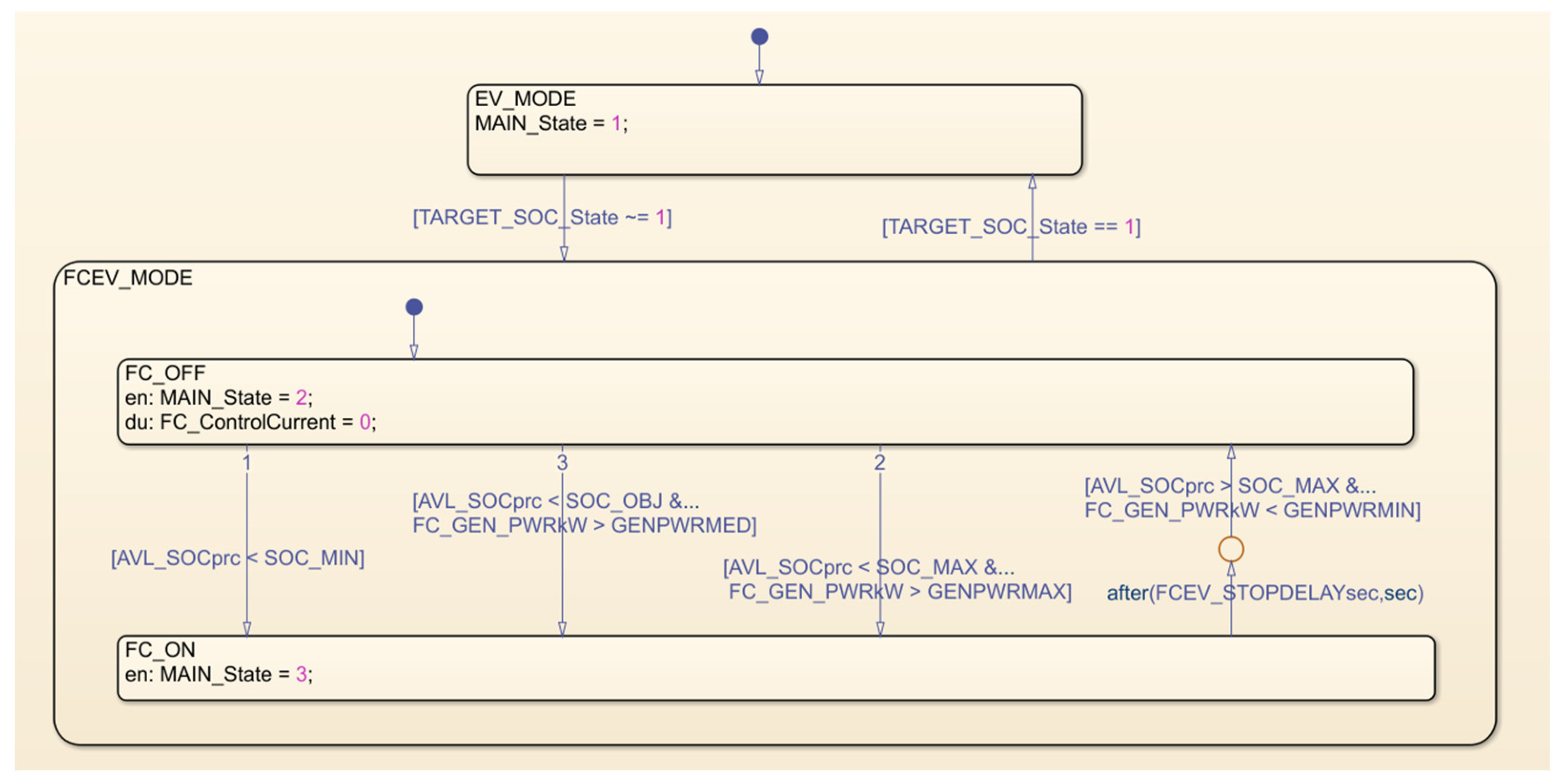
Additionally, an FSM is used to decide whether the generation unit (FC) shall be turned on or off, varying from EV-MODE and FC-MODE, depending on the battery pack SOC and the calculated power demand for the FC ($P_{FC}$). Specifically, the FC is always turned on when the SOC falls below a minimum value (${SOC}_{min}$), and it is turned off when it exceeds a maximum value (${SOC}_{max}$). In addition, in order to maintain a predefined target SOC, the FSM is further implemented to allow the FC to be switched on when the SOC is lower than a target value (${SOC}_{obj}>SO{C}_{min}$) but the $P_{FC}$ exceeds a certain threshold, thus aiming to achieve a high overall powertrain efficiency. Furthermore, the FC is also activated when the power demanded from the vehicle exceeds a threshold at which the aid of the hybrid part, in combination with the power available from the battery, is deemed convenient. Figure 2 shows the structure of the FSM for the presented PFCS.

For the first EMS, known as Standard Alternative PFCS (SA-PFCS), $P_{FC}$ is the power demanded to the FC when it is switched on. However, for the second EMS, known as the Discretized Alternative PFCS (DA-PFCS), up to six different levels of power demand to the FC are selected depending on the value of $P_{FC}$ when the FC is turned on. Thus, the DA-PFCS is just a discretization of the SA-PFCS that aims to reduce FC wearing and enhance durability, which could potentially be achieved using several constant operating points instead of directly following the $P_{FC}$ value. The SA-PFCS is the EMS used in the comparison between the two different models, the AVL Cruise M^TM and the MATLAB Simulink model, described in Section 6.

Both strategies allow for the utilization of the FC between the minimum load value of 15% and the maximum load value of 90%, thus excluding the areas with the lowest efficiency on the FC polarization curve. The DA-PFCS then discretizes the $P_{FC}$ values into six levels 15% apart, always selecting the one closest to the filtered $P_{D,Veh}$.

In this paper, simulations with both of the presented EMSs are carried out for a selected driving cycle. The results, shown in Section 7, are analyzed in order to determine the most convenient PFCS control strategy in terms of fuel consumption, electrical consumption, and durability for both the FC and the HV battery.

4. AVL Vehicle Model

AVL Cruise M^TM is a vehicle simulation software designed for mobility concept analysis, powertrain subsystem design, and virtual component integration, using high-quality real-time models from various domains, including engine, flow, aftertreatment, driveline, electrics, and hydraulics [19]. In this work, the software has been used to recreate the longitudinal dynamic behavior of a 27-tonne heavy-duty truck (Gross Vehicle Weight) for simulations with low computational costs and short execution times, while maintaining a high degree of reliability, which will be validated through comparison with a MATLAB-Simulink model.

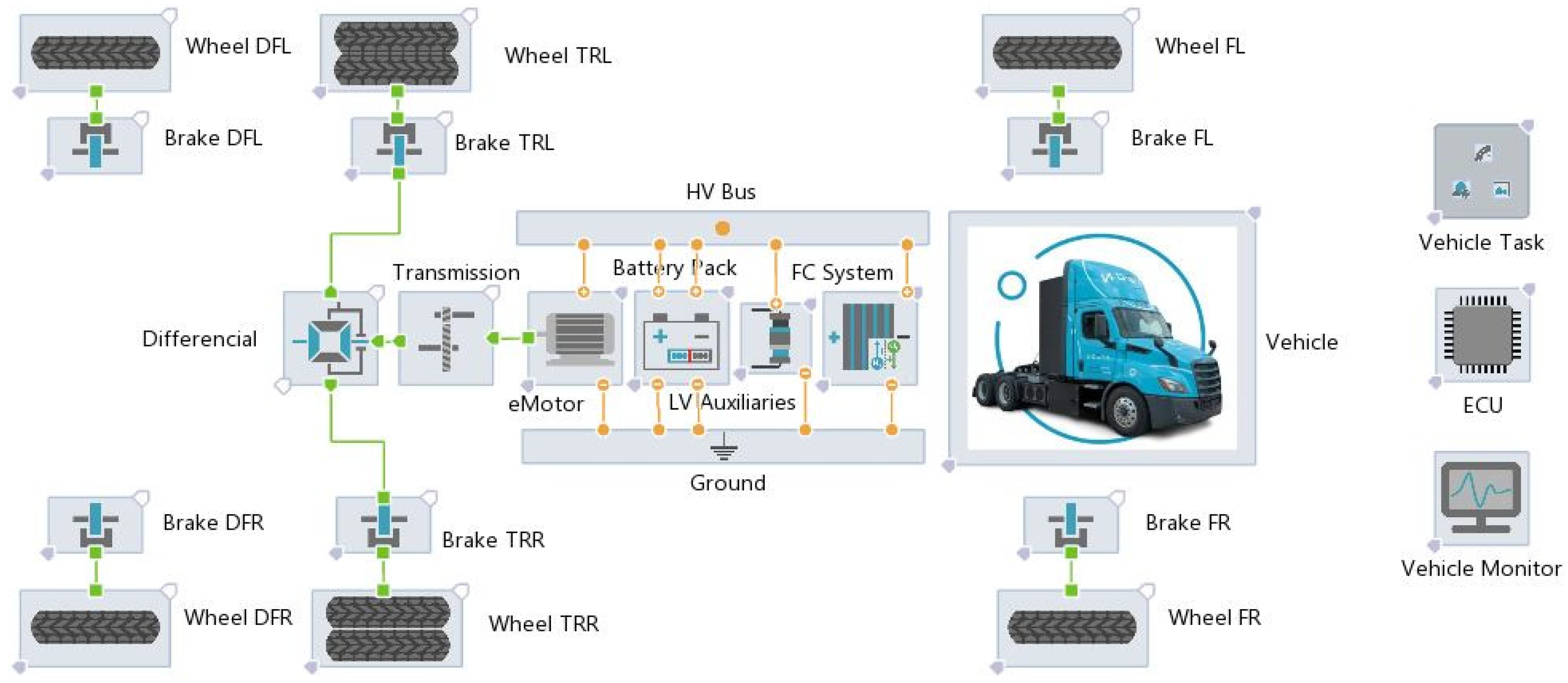
The complete powertrain structure of the selected fuel cell hybrid vehicle is shown in Figure 3. The hybrid architecture replicates a range-extender design, in which the HV battery is the main energy and power source, while the hybrid unit helps during transients and extends autonomy. The hybrid propulsion system can be seen in the center and uses an electric motor for traction, powered by an HV battery and a hydrogen hybrid unit. The vehicle consists of three axles, with the central drive axle visually connected to the propulsion system, unlike the other two.

This complete drive system in AVL Cruise M^TM is composed of a number of blocks, which are either actually part of the vehicle or not related to its structure but are necessary for the simulation.

4.1. High Voltage Battery

The model is based on an equivalent electric circuit and can predict the voltage response at a given current, SOC, and temperature. The parameterization involves entering the number of cells and modules, the minimum and maximum cell voltage, maximum charge (Ah), initial SOC, ohmic connection resistance during charge and discharge, and an open-circuit voltage (OCV) map. The data used in the parameterization of this component are those of the LiBESS cell ANR26650M1 in the A123 System battery [20] in the 200s72p configuration, which is required to achieve a capacity of 111.6 kWh (see

Table 1. LiBESS model parameters.

Parameter	Value	Aging Parameter	Value
Nominal capacity	7.74 Wh	c	0.0018
Nominal voltage	3.7 V	d	−1.85 × 100
Nº cells	14.400 (200s-72p)	e	0.0558
Internal resistance	6 mΩ per cell	f	5.22 × 106
a	2.09 × 108	g	0.6898
b	−1.22 × 10−5	h	−6.67 × 103

).

4.2. Electric Motor

The component present in AVL Cruise M^TM can be used to model electric motors using a simple map-based approach. Loss maps are also present, depending on the mechanical power, for both efficiency and heat. The electric motor tries to deliver the requested torque; then, the power losses are added to the mechanical power delivered to obtain the electrical power. The parameterization involves introducing the moment of inertia, the arrangement temperature, and several maps, including the full load torque characteristic in both the traction and regenerative quadrants, as well as efficiency maps for both quadrants. The data for this electric motor refers to a commercial 350 kW peak power PMSM DANA [21].

4.3. Fuel Cell System

The model, shown in Figure 4, which includes the FC and the DC/DC converter, is based on electrochemical equations derived from the cathode polarization curve of a PEM. The approximate solution of the equations considers the oxygen and proton transport losses in the catalytic layer of the cathode, as well as the oxygen losses in the gas diffusion layer, for different temperatures, relative humidity, and gas pressure. A simple compressor model is included in the fuel cell block so that the energy consumption of the compressor is measured as a function of the power consumed.

The parameterization involves entering various numerical values that are necessary for the definition of the polarization curve, the operation of the compressor, the chemistry present on the anode and cathode sides, and the thermal behavior. The data for this FC are taken from a commercial fuel cell stack, Ballard FCmove^TMHD, with a net output power of 100 kW [22]. Further details about these components’ characteristics cannot be provided because of a confidentiality agreement.

The DC/DC power converter regulates the current imposed on the load side of the FC, as shown in Figure 4. It also extracts the demanded power from the supply side to the load side to maintain the balance between input, output, and loss powers. There are two types of converter blocks in Cruise M; the one used at the output of a FC is the so-called “target current control” setting, which is defined as follows:

$$V_1·I_1·eff=V_2·I_{target}$$

(4)

Subscript 1 and 2 represent the two different sides of the converter (the supply and FC side, respectively), while $eff$ is its efficiency, whose value can be found in

Table 2. FCS model parameters.

Dynamic Parameter	Value
Power	100 kW
Nº cells	560
Nominal efficiency	50%
Operating Tª	65 °C
Voltage (at 0 A)	562 V

.

4.4. The Rest of the Model Elements

The wheel block is used to simulate wheel characteristics and calculate rolling resistance. It requires several data points and parameters, such as radius and wheel inertia, whose values can be found in

Table 3. Hybrid fuel cell–battery heavy-duty truck: simulation parameters.

Traction Machine		Fuel Cell
Type	PMSM	Type	PEM
Power	345 kW	Power	107 kW
Speed	1823 rpm	Voltage nom/max	450/314.6 VRMS
Torque	1807 Nm	Current nom/max	120/338.3 ARMS
Voltage	750 VRMS	nº cells	560
I_DC current	500 ARMS	DC/DC converter
Torque constant	1.4 Nm/A_peak	Type	IGBT module (1 branch)
Rs	0.02171 Ω	L = 2 mH	C = 1 mF
Ls	112 mH	Switch. freq.	25 kHz
Power converters (inverter)		Batteries
Type	IGBT module	Type	LFP (200s-72p))
DC voltage	750 VDC	Voltage (total)	740 V (3.7V × 200)
Current	500 ARMS	Current (C = 1)	165.6 A (2.3A × 72)
Switch. freq.	5 kHz	Capacity C = 1	111.541 kWh
Emulated FCEV		Aerodynamics and rolling
Type	Heavy-Duty Truck	Air density ρ	1.134 kg/m3
Gross vehicle mass (GVM)	27,000 kg	AF	8.37 m2
Total Inertia (at motor shaft)	112.61 kgm2	CD	0.7
ERR	0.491 m	µroll,0	0.0137
iGEAR	6.568	µroll,S	0.0110
µGEAR	95%

.

The brake block is used to simulate the braking characteristics of each wheel and is described by parameters such as piston surface, friction coefficient, effective braking radius, and disk inertias.

The differential block is set to compensate for discrepancies in the rotational rates of the driving wheels and requires the inertia values of the connected elements.

The transmission block is a single-ratio element that models a gear step with a fixed ratio considering constant efficiency. It can be used as a transmission step in a differential, creating the final drive unit.

The LV auxiliaries are treated as an energy consumer, which is represented as an electrical resistor consuming a user-defined amount of power. This approach simulates the consumption of the vehicle’s LV electrical auxiliaries, which for this vehicle were estimated to have an average value of 6.5 kW throughout the driving cycle.

The vehicle task block is a subsystem containing the driving cycle definition and configuration blocks for the driver (a PID controller) and environment parameters, whose values can be found in Table 3.

The vehicle block contains various parameters, such as weight, dimensions (wheelbase, distances to the center of gravity, etc.), frontal area value, and aerodynamic coefficient, among others, whose values can be found in Table 3.

The ECU subsystem contains blocks for the control of the traction system, such as maps, functions, and constants. The control strategy is described in Section 3.

Finally, the vehicle monitor block allows the user to decide which variables and trends to display in real time during a given simulation.

By configuring all elements appropriately and as realistically as possible, while referring to the vehicle specifications and individual element data sheets, it is possible to obtain simulations that represent the longitudinal dynamics of the vehicle with a certain degree of reliability. For this purpose, it is necessary to include a speed profile that the vehicle must follow and replicate. The results that can be obtained include the values and trends of all mechanical, physical, electrical, and chemical characteristics of all the elements that make up the model.

4.5. Driving Cycle

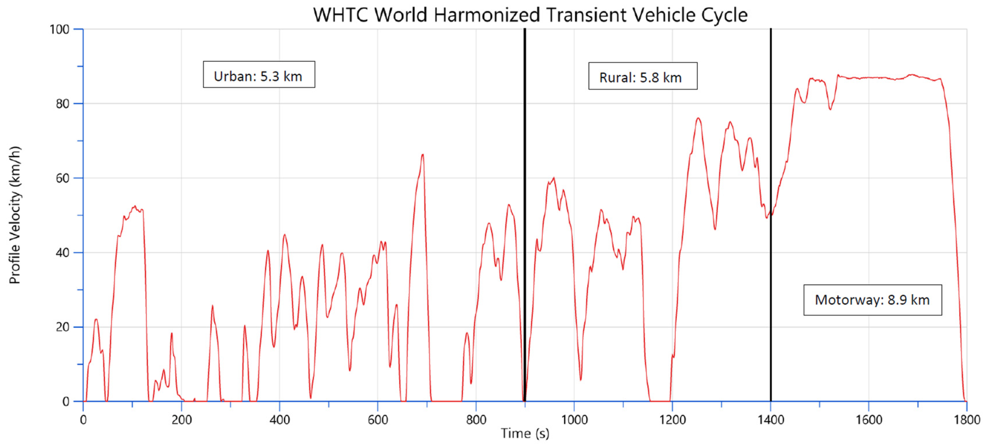
The driving cycle used in this work is the World Harmonized Transient Cycle (WHTC), which was created to reflect the operation of heavy-duty engines on the road worldwide, in relation to the globally harmonized technical regulation covering the type-approval procedure for exhaust emissions from heavy-duty engines [23]. The WHTC is a transient engine dynamometer schedule defined by the proposed Global Technical Regulation (GTR) developed by the UN ECE GRPE group. This cycle, shown in Figure 5, has been selected because it represents a driving standard for the vehicle under study, offering a variety of conditions (urban and extra-urban) throughout its duration.

5. MATLAB-Simulink System Model

In order to validate the results obtained from the simulation model developed in the AVL environment, a second computer model of the heavy-duty FCEV powertrain has been developed in MATLAB Simulink^®. This new model represents the same powertrain of the hybrid fuel cell–battery vehicle, including all the components discussed in Section 4, but with greater detail in certain parts compared with the AVL model. For example, both power converters and the traction motor have been simulated using their model equations instead of their operational curves derived from the manufacturer data sheets. The controls the models used in this simulation environment are especially robust and simple; however, since the electronic converters are represented in detail, a very short cycle time must be used to deal with the commutation frequency, thus allowing for the acquisition of, for example, real currents with their ripple. 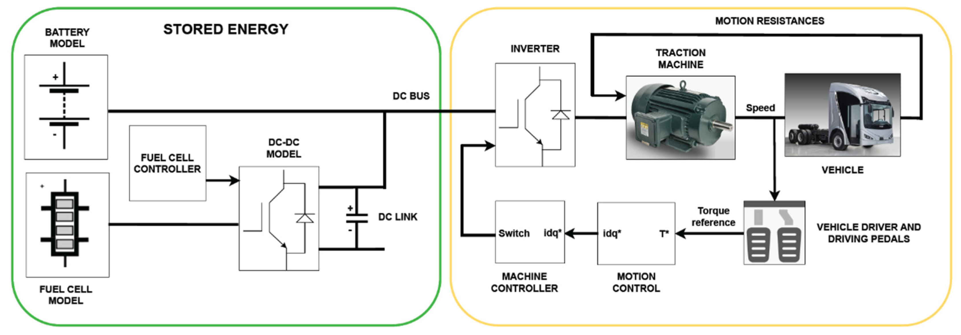Figure 6 shows a diagram of the main model layer.

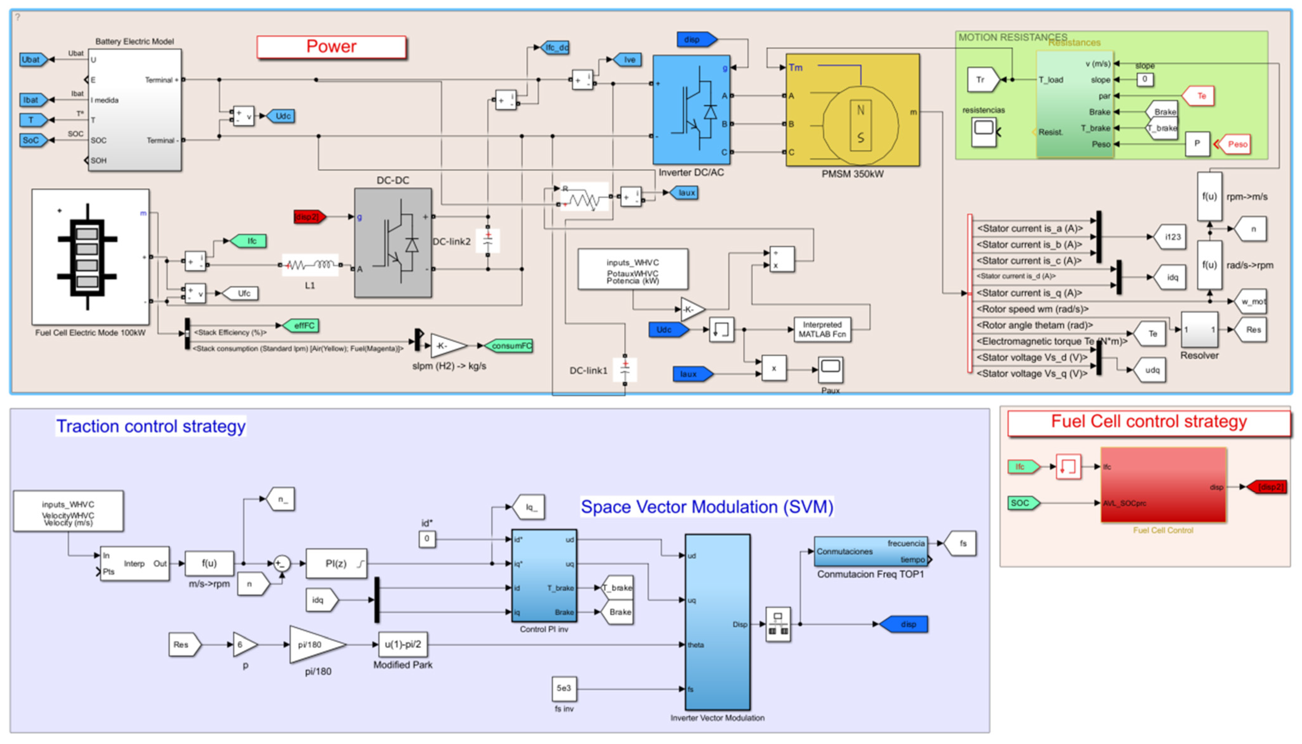
The model consists of two primary components, as shown in Figure 6. The energy storage section on the left comprises the battery, fuel cell, DC/DC converter, and its associated control system. The motor section on the right encompasses the inverter, traction machine, control system, and the vehicle itself, which is represented as an equivalent load in terms of mass, inertia, and motion resistance.

The subsequent sections outline the mathematical models incorporated within each block of Figure 6, moving from left to right.

5.1. Battery Stack

The Li-ion battery energy storage system (LiBESS) model is an adaptation of the generic battery model available in the SimPower Systems library of Simulink, initially proposed in (Tremblay and Dessaint, 2009 [24]). This specific LiBESS model was chosen for its user-friendliness, accuracy (despite its simplicity), and dynamic performance.

The dynamic (runtime) and thermal behavior of the model have been modified, and a detailed explanation and validation is included in [25]. The version presented here differs from the one in [24] in that it sacrifices some generality for simplicity because it is specifically designed for lithium-ion batteries. Additionally, the internal resistance is represented by two distinct electrical resistances: a constant ohmic resistance and a variable polarization resistance that depends on the state of charge (SOC).

Additionally, the aging model included in the Simulink library has been replaced by a more accurate model, which was previously developed and validated in [26]. This aging model measures the LiBESS lifetime in terms of capacity decay and is valid for both LFP and NMC chemistries within Li-ion. The model considers both cycling and calendar aging, and it has been implemented in an online manner, meaning that the dynamic and thermal parameters of the model vary as the LiBESS ages. The main equation of the model is included as follows:

$$Q_{loss}=\left(a·T^2+b·T+c\right)·e^{\left(d·T+e\right)·C_{rate}}·\mathrm{A}\mathrm{H}+\mathrm{f}·e^{g·SoC}·e^{{\displaystyle \frac{h}{T}}}·{\mathrm{t}}^{\mathrm{z}}$$

(5)

where $Q_{loss}$ denotes the final capacity degradation in percentage, $T$ represents the battery temperature in Kelvin, $AH$ stands for the ampere-hour throughput in Ah, $C_{rate}$ is the charge/discharge rate, $t$ represents the time in days, z is the power law factor, and the constants a through h are parameters that depend on the battery’s chemistry.

The models, all dynamic, thermal, and aging, have been parameterized based on the LiBESS cell ANR26650M1 from A123. The main parameters are included in Table 1, where parameters a to h correspond to the aging model.

5.2. Fuel Cell Stack

The fuel cell stack (FCS) model is based on the model included in the Specialized Power Systems library of Simulink provided by MathWorks [27]. The model has not been modified in terms of open-circuit voltage operation (dynamic operation); however, an offline aging model has been included to estimate the lifetime of the FCS. This model is described and validated in [28] and allows for measuring the aging associated with the FCS in terms of cell voltage degradation.

From a general perspective, the voltage degradation of the FCS is evaluated based on its operation modes, which are as follows:

• FCS operated in an open circuit (OCV mode).
• FCS shuts down when the power falls below a specific limit (SSC mode).
• FCS working with constant voltage (CA mode).
• FCS operated with voltage cycles (VC mode).

The FCS voltage degradation is calculated for each mode independently (no coupling between modes is considered) and then added as follows:

$$∆U_{total}=∆U_{OCV}+∆U_{SSC}+∆U_{VC}+∆U_{CA}$$

(6)

Equations affecting variables and parameters for computing the FCS aging associated with each mode are described in [28]. The FCS models, including dynamic and aging, have been parameterized based on the 100 kW FCS FCmove™ HD+ E/R1.1. The parameters are summarized in Table 2.

5.3. DC/DC Converter and DC Link

The models for the power electronics converters are also derived from power semiconductors found in the SimPowerSystems library [29]. The power components utilized in this study are from the IGBT module “SEMiX453GD12E4c” [30].

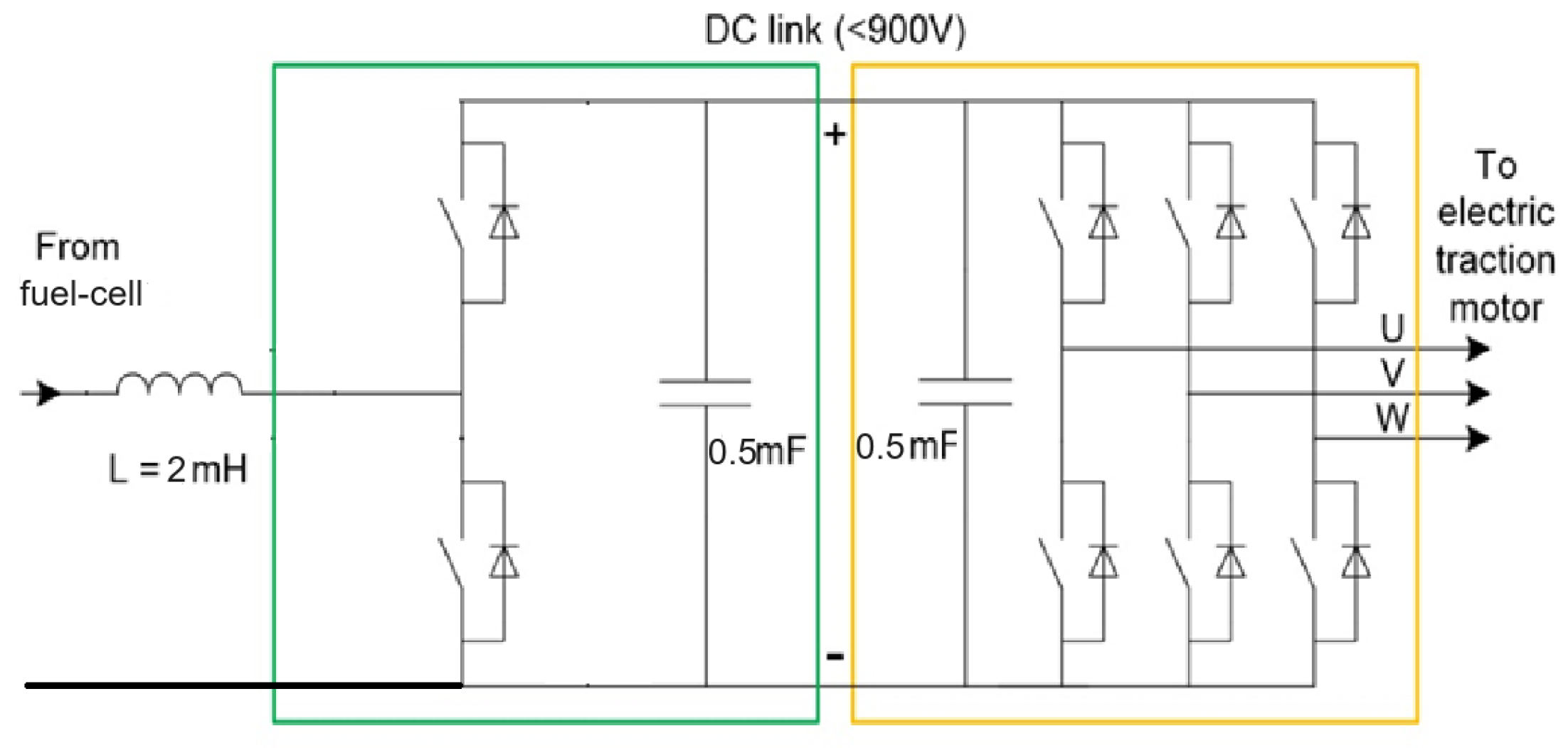
Although in this application the converter only works in one way, the DC/DC converter that has been modeled can function as a bidirectional buck-boost converter [31], connecting to the fuel cell by means of an inductance (2 mH), as shown in Figure 7.

Finally, the DC link consists of a set of capacitors (1100 V, 0.5 mF) connected in parallel, resulting in an equivalent total capacitance of 1 mF.

5.4. Inverter

The DC/AC converter is modeled in the same manner as the DC/DC converter. However, in this instance, the converter operates as a standard three-phase current-controlled voltage source inverter (VSI), as depicted in Figure 7 [32].

5.5. Traction Machine

The selected vehicle’s motor is a 350 kW permanent magnet synchronous machine (PMSM). The electric motor model is based on data extracted from the manufacturer [21] and from the literature [33,34,35].

The equations used in the model are as follows [36] (amplitude-invariant Clarke transformation) [37]:

$$\left[\begin{array}{c}{u}_d\\ u_q\end{array}\right]=R_S·\left[\begin{array}{c}{i}_d\\ i_q\end{array}\right]+{\displaystyle \frac{d}{dt}}\left[\begin{array}{c}{\lambda }_d\\ {\lambda }_q\end{array}\right]+{\omega }_{elec}·\left[\begin{array}{cc}0& -1\\ 1& 0\end{array}\right]·\left[\begin{array}{c}{\lambda }_d\\ {\lambda }_q\end{array}\right]$$

(7)

$$T_{em}={\displaystyle \frac{3}{2}}·p·\left({\lambda }_d·i_q-{\lambda }_q·i_d\right)$$

(8)

$$T_{em}-T_{load}=J·{\displaystyle \frac{d{\omega }_{mec}}{dt}}+\mathrm{B}·{\omega }_{mec}$$

(9)

where

• u_d, u_q: stator voltages in dq reference frame [V].
• p: pole pairs [-].
• i_d, i_q: stator currents in dq reference frame [A].
• T_load: load torque [Nm].
• R_S: stator winding resistance [Ω].
• ω_elec: rotor electrical speed [rad/s].
• T_em: electromagnetic torque [Nm].
• J: total moment of inertia [kg·m²].
• ω_mec: rotor mechanical speed [rad/s].
• B: total friction [Nm/(rad/s)].
• λ_d, λ_q: stator flux linkages in dq reference frame [Wb].

5.6. Vehicle and Motion Resistances

The vehicle model captures both the inertia of the vehicle and its resistance to motion. These resistances include rolling resistance, aerodynamic drag, and gradient resistance (which can be either positive or negative). Transmission losses are also considered. The three types of motion resistance are modeled as follows [33]:

$$F_T=F_{aero}+F_{roll}+F_{grav}$$

(10)

$$F_{aero}={\displaystyle \frac{1}{2}}·\rho ·A_F·C_D·{(v-v_{WIND})}^2\ge 0$$

(11)

$$F_{roll}={\mu }_{roll}·M·g·\mathrm{c}\mathrm{o}\mathrm{s}\left(\alpha \right)>0$$

(12)

$$\mathrm{with} {\mu }_{roll}={\mu }_{roll,0}+{\mu }_{roll,S}·v^{2.5}$$

(13)

$$F_{grav}=M·g·\mathrm{s}\mathrm{i}\mathrm{n}\left(\alpha \right)\gtrless 0$$

(14)

where

• F_T: total motion resistance [N].
• M: total mass of the vehicle [kg].
• F_aero: aerodynamic resistance [N].
• µ_roll: rolling resistance coefficient [-].
• F_roll: rolling resistance [N].
• µ_roll,0: constant rolling resistance coefficient [-].
• F_grav: gradient resistance [N].
• µ_roll,S: incremental rolling resistance coefficient [-].
• ρ: air mass density [kg/m³] α: road slope (positive when climbing) [º].
• A_F: vehicle frontal area [m²].
• g: free fall acceleration [m/s²].
• C_D: vehicle drag coefficient [-].
• v: vehicle speed [m/s].
• v_wind: headwind speed (positive in the same direction than the vehicle) [m/s].

The load torque in (9) is calculated from the total motion resistance in (10) using the following expression:

$$\left\{\begin{array}{c}{T}_{load}={\displaystyle \frac{ERR}{i_{GEAR}·{\mu }_{GEAR}}}·F_T (traction mode)\\ T_{load}={\displaystyle \frac{ERR·{\mu }_{GEAR}}{i_{GEAR}}}·F_T (regenerative mode)\end{array}\right.$$

(15)

where ERR [m] represents the effective rolling radius (distinct from the loaded tire radius) [38], i_GEAR [-] is the transmission gear ratio, and µ_GEAR [-] denotes the transmission energy efficiency (assumed to be constant at 0.95) [39]. Regarding the moment of inertia, the total inertia J_vehicle [kg·m] as experienced by the electric motor is given as follows:

$$J_{vehicle}=J_{high}+{\displaystyle \frac{J_{low}}{{i_{GEAR}}^2}}+{\displaystyle \frac{M·{ERR}^2}{{i_{GEAR}}^2}}$$

(16)

where J_high and J_low are the total rotational inertia in the high-speed shaft (motor shaft) and low-speed shaft (wheel shaft), respectively. The majority of the vehicle’s inertia is determined by its mass M. The parameter values used in Equations (10)–(16) for the simulated vehicle are listed in Table 3.

5.7. Control Strategies and Power Converter Modulation

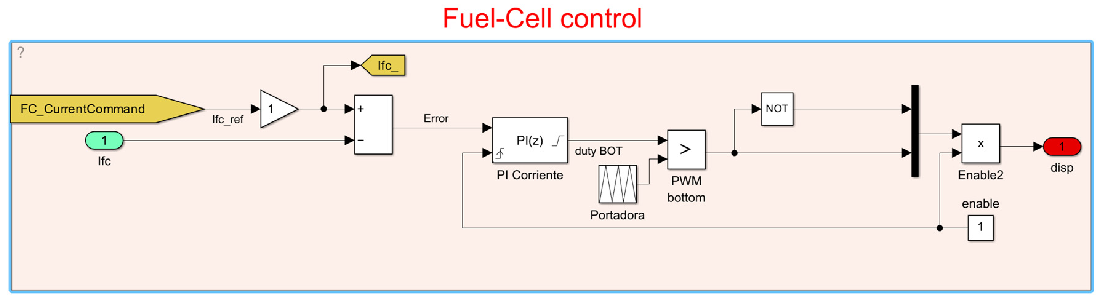
The DC/DC converter adapts the fuel cell voltage to the DC bus voltage, which is set by the battery, while controlling the current extracted from the fuel cell.

The DC/DC control is dedicated to keeping the fuel cell current close to its reference value, which is set by the Energy Management Strategy of the hybrid FC-battery vehicle. In Figure 8, the DC/DC converter control is presented in detail. The output is the pulse pattern, which will be used to trigger the bottom IGBT of the converter.

With respect to the inverter, the selected modulation strategy is conventional space vector modulation (SVM), which implies a constant switching frequency [32]. In Figure 9, the complete Simulink model is presented.

The machine control system operates on two levels. The upper level is the motion controller, which generates a current reference, [I_d*, I_q*], in dq coordinates (rotor reference frame for PMSM) based on the speed reference value (from the WHTC driving cycle) using a PI controller. The lower level, known as the machine controller, handles the modulation technique. In this block, [I_d*, I_q*] are compared to the actual motor currents, [I_d, I_q], and two PI regulators generate the voltage references, [V_d*, V_q*], that should be converted to a stationary reference for the SVM modulation. The firing signals coming from the SVM block control the three branches of the inverter feeding the motor. In this model, the current reference does not adhere to the MTPA trajectory shown in [33], so I_d* = 0 is used instead [36], without applying flux weakening above rated speed.

Table 3 presents the main vehicle parameters used within the two simulation environments.

6. Validation of the AVL Model Relying on Sprague and Geers Validation Metric

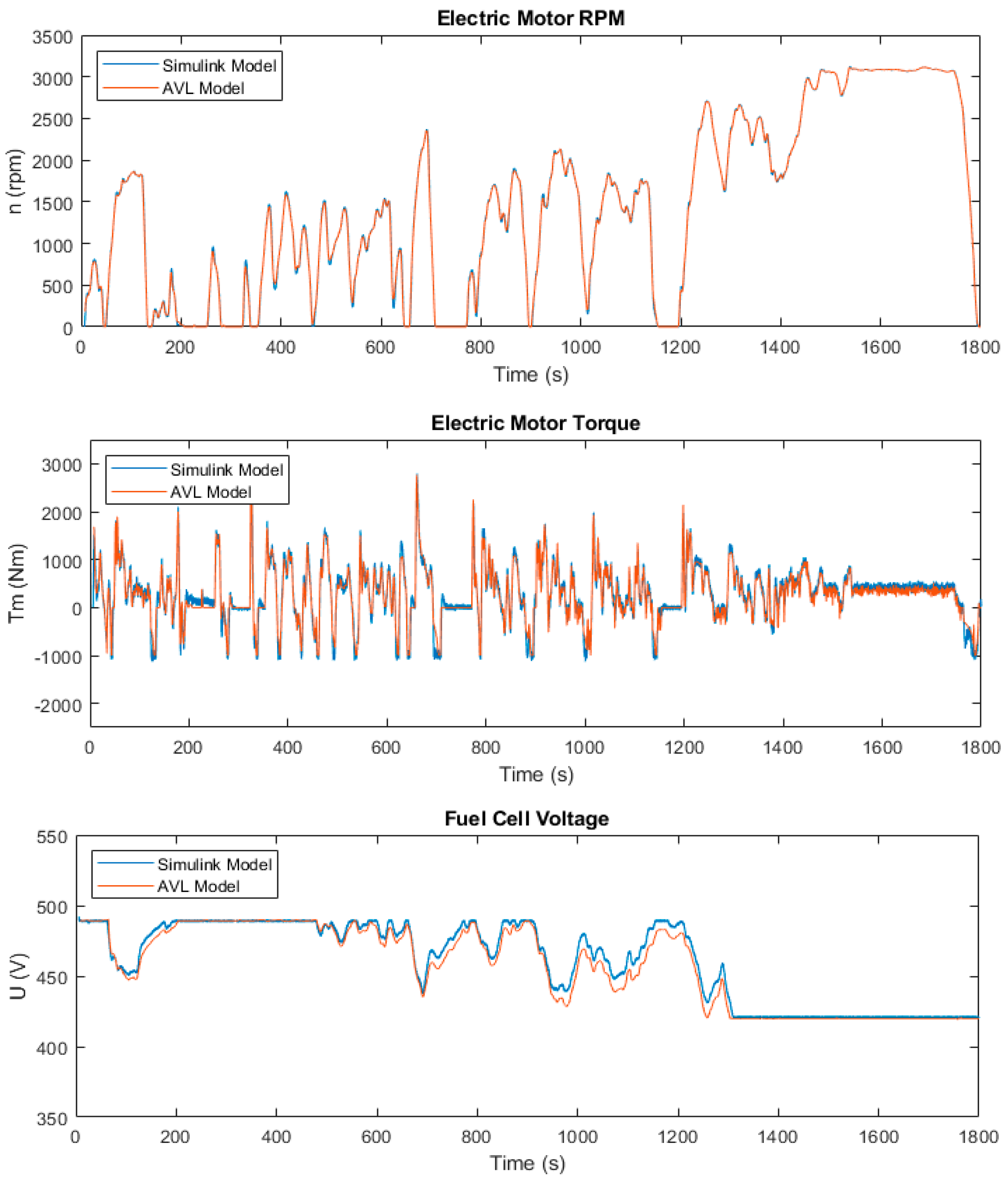
To verify that the AVL model accurately reproduces the behavior of the detailed model, a validation process using metrics has been followed. The selected metric is the Sprague and Geers metric, which is widely used for dynamic phenomena such as the one being modeled in this work. This metric has been thoroughly evaluated by Schwer [40] against Subject Matter Expert opinion, showing an excellent correlation. The only limitation mentioned is its asymmetry, with slightly different values depending on which data is chosen as the reference (b(t)) and which is the function to compare (c(t)). In Figure 10, some powertrain variables of the selected FCEV following a WHTC cycle, using both AVL and MATLAB simulation models, are presented as an example to show the similarities between the results obtained with them, along with the weight of the fully loaded vehicle. From top to bottom, the time diagrams of the following variables are compared in the figure: Electric Motor Speed, Electric Motor Torque, Fuel Cell Voltage, Fuel Cell Current, HV Battery Voltage, and HV Battery Current. In this comparison, the fuel cell is used in both models based on the SA-PFCS described in Section 3.

To assess the degree of approximation of the results obtained from the AVL simulation model and the MATLAB validation tests, the Sprague and Geers validation metric [40] has been used. This metric proposes a quantitative method for assessing the similarity of two signals, c(t) and b(t), by obtaining two coefficients, M and P, which quantify, respectively, the discrepancies between the signals in magnitude M (17) and in phase (18). Based on the results of the abovementioned errors, the metric proposes a combined error, C, calculated as the root mean square of M and P. The closer the results of the parameters P, M, and C are to 0, the higher the similarity between the compared historical data.

$$M=\sqrt{{\vartheta }_{cc}/{\vartheta }_{bb}}-1$$

(17)

$$P={\displaystyle \frac{1}{\pi }}{cos}^{-1}\left({\vartheta }_{bc}/\sqrt{{\vartheta }_{bb}{\vartheta }_{cc}}\right)$$

(18)

$$C=\sqrt{M^2+P^2}$$

(19)

where:

$${\vartheta }_{bb}={(t_2-t_1)}^{-1}{\int }_{t_1}^{t_2}{b}^2\left(t\right)dt$$

(20)

$${\vartheta }_{cc}={(t_2-t_1)}^{-1}{\int }_{t_1}^{t_2}{c}^2\left(t\right)dt$$

(21)

$${\vartheta }_{cc}={(t_2-t_1)}^{-1}{\int }_{t_1}^{t_2}b\left(t\right)c\left(t\right)dt$$

(22)

For the comparison of the signals, the metric analysis has been performed by estimating all values from t₁ = 0 to t₂ = t, where t is any value less than or equal to the final time of the simulations. This systematic approach allowed us to obtain an evolution of the metric throughout the simulation, rather than a single final value considering the whole time interval.

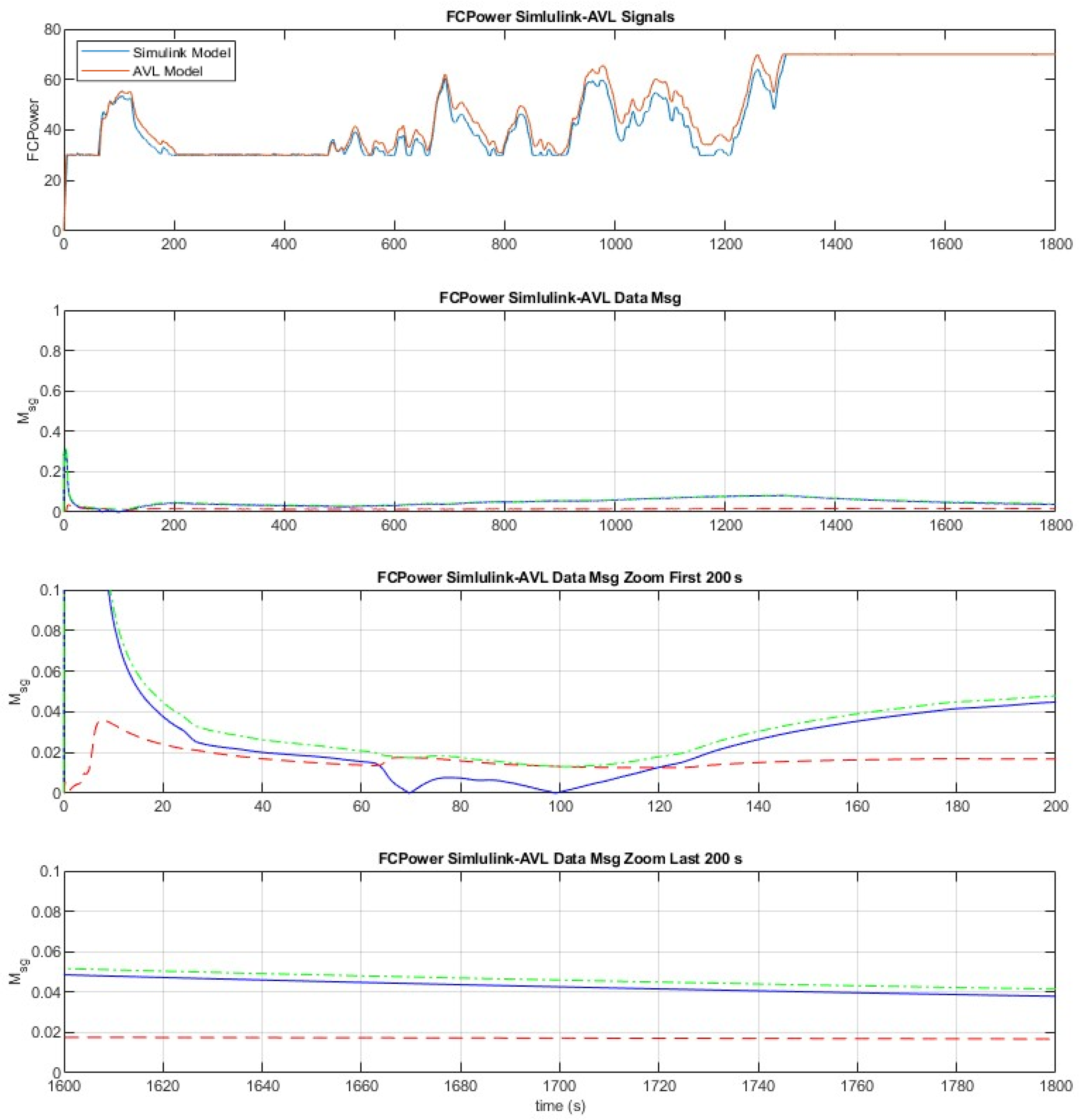
The application of the metric has been conducted using a MATLAB routine that generates graphs to assess the quality of the fitness between the two models. The code automatically generates graphs, such as those presented in Figure 11, which are an example of the application relying on the fuel cell power profile throughout the cycle and are outlined as follows:

• Comparison of model signals over the entire simulated time range.
• Metric results displayed on a normalized scale (0 to 1) with error types (M in blue, P in red, C in green).
• Metric results for the time interval 0–200 s, with the error axis scaled to 10%.
• Metric results for the last 200 s, with the error axis scaled to 10%.

The parameters used to contrast the results between the two models, as well as the aggregate value of the metric over the entire simulated period (1800 s), are presented in

Table 4. Compared parameters for the validation of the AVL simulation model.

Name	Description	M	P	C
BatteryPackCurrent_SAData_Msg	I/O current of the battery pack	10.1%	9.3%	14.30%
eMCurrent_SAData_Msg	Electric motor current	7.60%	7.60%	10.10%
eMTorque_SAData_Msg	Electric motor torque	6.00%	6.90%	9.20%
FCVoltage_SAData_Msg	Fuel cell voltage	8.10%	2.90%	8.60%
BatteryPackPower_SAData_Msg	I/O power of the battery pack	4.00%	7.00%	8.00%
ElectricalPower_SAData_Msg	I/O DC bus power	1.30%	6.20%	6.30%
Current_SAData_Msg	I/O DC bus current	4.80%	2%	5.20%
FCPower_SAData_Msg	Fuel cell power	3.8%	1.7%	4.10%
Speed_SAData_Msg	Electric motor speed	0.16%	0.49%	0.50%
StateOfCharge_SAData_Msg	Battery state of charge	0.40%	0.24%	0.47%
FCEfficiency_SAData_Msg	Fuel cell efficiency	0.28%	0.10%	0.30%
Voltage_SAData_Msg	DC bus voltage	0.07%	0.05%	0.09%

.

The differences between the models are under 15% for all parameters. Ten of the twelve parameters show differences of under 10%, with the only exception being the I/O current of the Battery Pack (10.8%). Based on the results obtained, it can be concluded that both models reproduce the dynamics of the powertrain with the same level of accuracy, making it possible to validate and consider the results of the AVL model to be reliable, which will be used to compare the different EMSs.

7. Comparison Between the Two Selected EMSs

The two selected EMS presented in Section 3, Standard Alternative PFCS (SA-PFCS) and Discretized Alternative PFCS (DA-PFCS), have been studied using the models presented in Section 4 and Section 5 of this paper. The comparison between both strategies has been made in terms of hydrogen and energy consumption, as well as degradation in both the battery and the fuel cell caused by each strategy. The simulation was performed during a single WHTC driving cycle, with the weight of the fully loaded vehicle. To obtain the results for electricity and hydrogen consumption, we decided to simulate the longitudinal dynamics of the heavy-duty truck with an initial battery SOC of 50% to guarantee the operation of the fuel cell. In fact, in both EMSs, the FC activation is set when 50% of the battery’s state of charge is reached to allow for the inclusion of the dynamics of the FC startup in the simulation, which has consequences in terms of degradation.

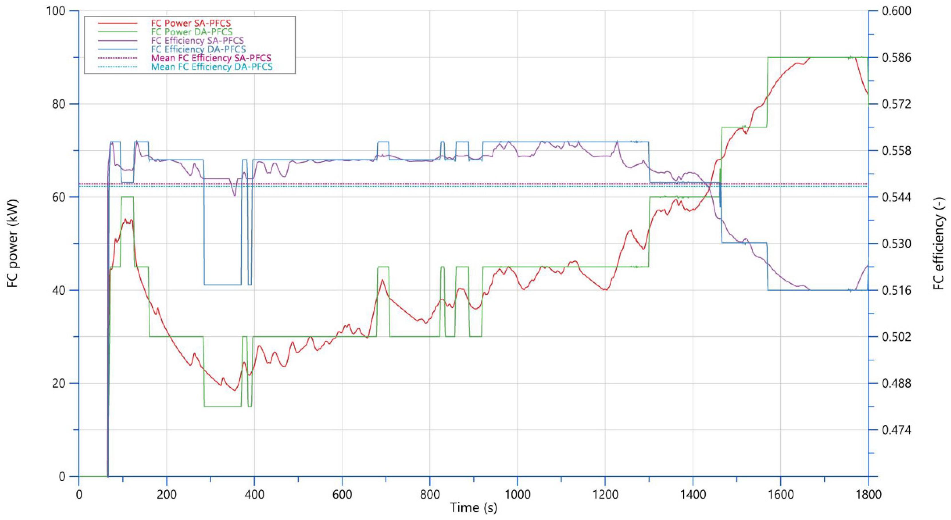
Figure 12 shows the different operating conditions of both strategies concerning fuel cell utilization, showing the differences in power trends (with and without the discretization of power levels) and efficiency, which is slightly higher on average for the SA-PFCS. The more discretized power profile of the DA-PFCS can be observed when compared to the SA-PFCS, which follows the average power demand of the vehicle over the WHTC cycle. The discretization is also reflected in the efficiency, which fluctuates among six values in the DA-PFCS (corresponding to those of the power).

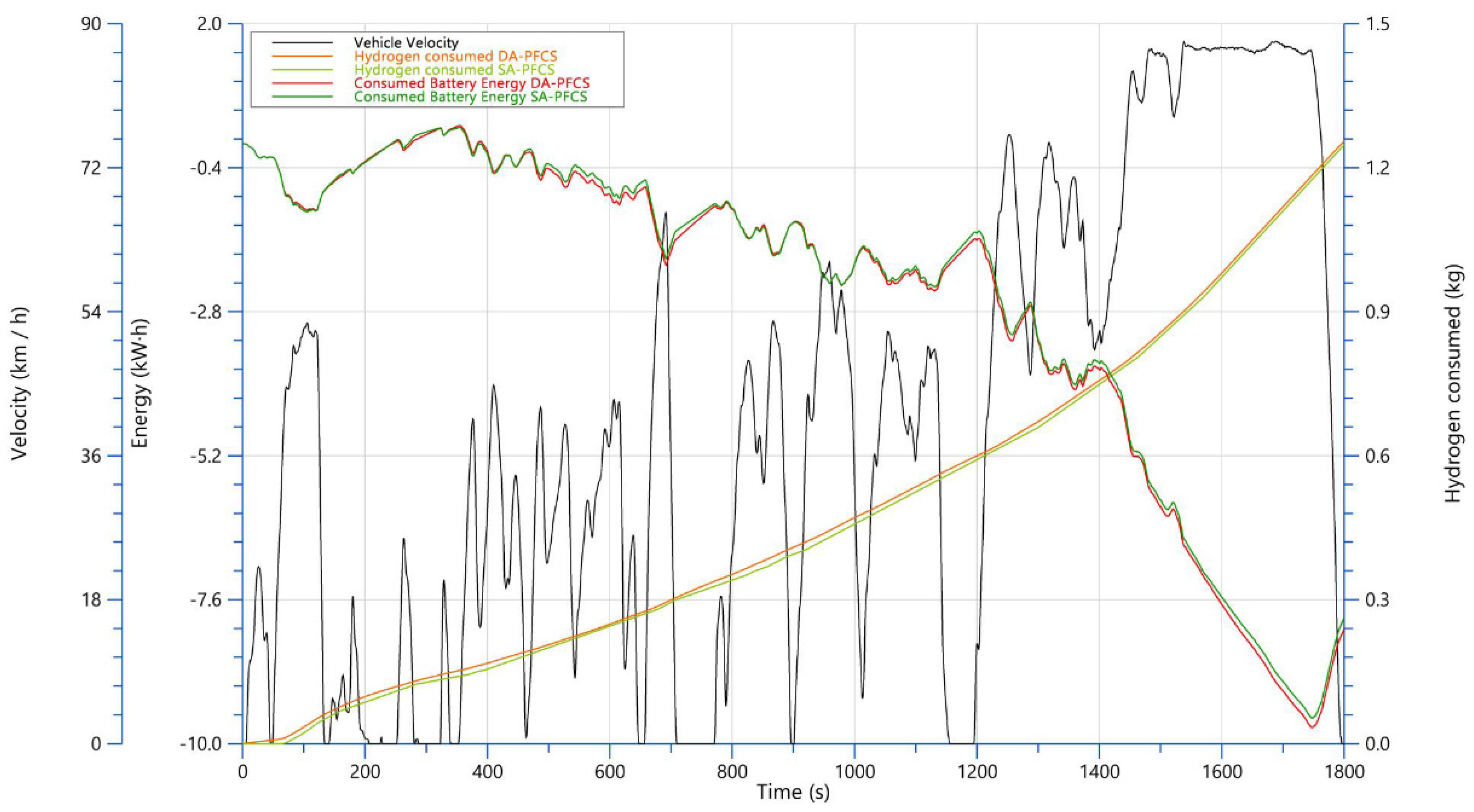
In Figure 13, the electrical energy and fuel consumption resulting from the selected vehicle simulation along the WHTC using both selected EMSs are presented in terms of battery energy and hydrogen consumption trends. It can be seen that the DA-PFCS generates higher final hydrogen consumption with lower electrical energy consumption compared to the SA-PFCS. The battery decreases its state of charge during the cycle, with the hybrid part consuming fuel while providing the average power of the cycle, especially in the final part that corresponds to the motorway section with higher velocities.

The results of the comparison between the two selected strategies in terms of consumption and degradation are summarized in

Table 5. Results in consumption and battery and FC degradation for the SA-PFCS and DA-PFCS EMSs.

Element	Variable	SA-PFCS	DA-PFCS	U.M.
Fuel Cell	H2 Consumption	1.247	1.255	kg
	Consumed Energy	22.815	22.920	kWh
	Voltage Degradation	0.00147	0.00141	%
	Mean Efficiency	0.548	0.547	[f-]
Battery	SOC Consumption	7.516	7.341	%
	Consumed Energy	8.100	7.903	kWh
	Voltage Degradation	0.0123	0.0117	%

. The translation of the results obtained with the model presented in this work to real costs exceeds the technical scope of this paper, since the costs of electricity, hydrogen, batteries, and fuel cells are rapidly changing and vary across different countries and companies.

To perform the battery degradation analysis, a recharge with a CC-CV profile was added at the end of the WHTC cycle to bring the battery back to 50% SOC, with a C-rate of 0.2C. This aspect was included because the current circulating in the battery at the time of charging is also a source of degradation for the latter and must be considered in a more refined analysis. On thfe other hand, regarding the FC, refueling does not represent a situation in which it experiences degradation.

From the results, it can be seen that the use of an SA-PFCS results in lower consumption for the FC in terms of fuel and energy, but at the cost of higher battery energy consumption. On the contrary, the use of the DA-PFCS presents the opposite trend, with higher consumption for the FC being reflected in lower battery energy consumption. Regarding degradation, the use of an SA-PFCS degrades both the FC and the battery more than the DA-PFCS.

8. Conclusions

This paper presents a multicriteria evaluation tool that enables the assessment of an FCEV powertrain’s performance under specific operating conditions—such as driving cycles—and the comparison of different EMSs based on overall costs, including operational consumption and system degradation. This tool is implemented in a methodology to select an EMS that minimizes both fuel cell and battery aging while reducing hydrogen and energy consumption in a heavy-duty FCEV.

The simulation model for performing the simulations across the methodology, developed in the AVL environment, has been validated using a more detailed MATLAB Simulink model. Semi-empirical aging models for the battery and fuel cell were incorporated into the simulation to evaluate EMSs in terms of system degradation.

To demonstrate the applicability of the proposed methodology, two EMSs were selected: a Standard Alternative Power Follower Control System (SA-PFCS) and a Discretized Alternative PFCS (DA-PFCS). Both EMSs are tested for a use case specific to commercial devices and a standard driving cycle.

Based on the comparison conducted using this methodology with the two EMSs presented as examples, it can be concluded that if the goal is to reduce hydrogen consumption, a SA-PFCS is preferable, whereas if the aim is to preserve both the battery and fuel cells to extend their lifespan, a DA-PFCS is the better option.

These findings demonstrate the practical value of the proposed tool and methodology in supporting the design and optimization of EMSs for heavy-duty FCEVs, paving the way for improved performance and an enhanced ESS lifespan.

References

- Sorlei, I.-S.; Bizon, N.; Thounthong, P.; Varlam, M.; Carcadea, E.; Culcer, M.; Iliescu, M.; Raceanu, M. Fuel cell electric vehicles—A brief review of current topologies and energy management strategies. Energies 2021, 14, 252. [Google Scholar] [CrossRef]
- Kök, C.; Mert, S.O. Comparison of energy and exergy analysis of fuzzy logic and power follower control strategies in fuel cell electric vehicles. J. Power Sources 2024, 614, 235033. [Google Scholar] [CrossRef]
- Wu, J.; Peng, J.; Li, M.; Wu, Y. Enhancing fuel cell electric vehicle efficiency with TIP-EMS: A trainable integrated predictive energy management approach. Energy Convers. Manag. 2024, 310, 118499. [Google Scholar] [CrossRef]
- Jiang, Q.; Béthoux, O.; Ossart, F.; Berthelot, E.; Marchand, C. A comparison of real-time energy management strategies of FC/SC hybrid power source: Statistical analysis using random cycles. Int. J. Hydrogen Energy 2021, 46, 32192–32205. [Google Scholar] [CrossRef]
- Ferrara, A.; Jakubek, S.; Hametner, C. Energy management of heavy-duty fuel cell vehicles in real-world driving scenarios: Robust design of strategies to maximize the hydrogen economy and system lifetime. Energy Convers. Manag. 2021, 232, 113795. [Google Scholar] [CrossRef]
- Novella, R.; Plá, B.; Bares, P.; Pinto, D. Online Model Adaption for Energy Management in Fuel Cell Electric Vehicles (FCEVs). Appl. Sci. 2024, 14, 3473. [Google Scholar] [CrossRef]
- Han, R.; He, H.; Zhang, Z.; Quan, S.; Chen, J. A multi-objective hierarchical energy management strategy for a distributed fuel-cell hybrid electric tracked vehicle. J. Energy Storage 2024, 76, 109858. [Google Scholar] [CrossRef]
- Gu, H.; Yin, B.; Yu, Y.; Sun, Y. Energy management strategy considering fuel economy and life of fuel cell for fuel cell electric vehicles. J. Energy Eng. 2023, 149, 04022054. [Google Scholar] [CrossRef]
- Tran, D.-D.; Vafaeipour, M.; El Baghdadi, M.; Barrero, R.; Van Mierlo, J.; Hegazy, O. Thorough state-of-the-art analysis of electric and hybrid vehicle powertrains: Topologies and integrated energy management strategies. Renew. Sustain. Energy Rev. 2020, 119, 109596. [Google Scholar] [CrossRef]
- Ragab, A.; Marei, M.I.; Mokhtar, M. Comprehensive Study of Fuel Cell Hybrid Electric Vehicles: Classification, Topologies, and Control System Comparisons. Appl. Sci. 2023, 13, 13057. [Google Scholar] [CrossRef]
- Li, Q.; Yang, H.; Han, Y.; Li, M.; Chen, W. A state machine strategy based on droop control for an energy management system of PEMFC-battery-supercapacitor hybrid tramway. Int. J. Hydrogen Energy 2016, 41, 16148–16159. [Google Scholar] [CrossRef]
- Kim, M.; Jung, D.; Min, K. Hybrid thermostat strategy for enhancing fuel economy of series hybrid intracity bus. IEEE Trans. Veh. Technol. 2014, 63, 3569–3579. [Google Scholar] [CrossRef]
- Trinh, H.-A.; Truong, H.-V.; Ahn, K.K. Development of Fuzzy-Adaptive Control Based Energy Management Strategy for PEM Fuel Cell Hybrid Tramway System. Appl. Sci. 2022, 12, 3880. [Google Scholar] [CrossRef]
- Xu, W.; Liu, M.; Xu, L.; Zhang, S. Energy Management Strategy of Hydrogen Fuel Cell/Battery/Ultracapacitor Hybrid Tractor Based on Efficiency Optimization. Appl. Sci. 2022, 13, 151. [Google Scholar] [CrossRef]
- Musardo, C.; Rizzoni, G.; Guezennec, Y.; Staccia, B. A-ECMS: An adaptive algorithm for hybrid electric vehicle energy management. Eur. J. Control. 2005, 11, 509–524. [Google Scholar] [CrossRef]
- Álvarez Sánchez, J. Estrategias de Control Mediante MPC para un Vehículo Autónomo con Control de Derrape. Bachelor’s Thesis, UPM, Madrid, Spain, 2021. [Google Scholar]
- Xu, L.; Li, J.; Ouyang, M.; Hua, J.; Yang, G. Multi-mode control strategy for fuel cell electric vehicles regarding fuel economy and durability. Int. J. Hydrogen Energy 2014, 39, 2374–2389. [Google Scholar] [CrossRef]
- Álvarez Sánchez, J. Estrategias de Gestión de la Energía en Vehículos Híbridos y Programación de la Unidad de Control Principal de un Vehículo Pesado Híbrido Serie. Master’s Thesis, UPM, Madrid, Spain, 2023. [Google Scholar]
- AVL Cruise M. AVL. (n.d.). Available online: https://www.avl.com/en/simulation-solutions/software-offering/simulation-tools-a-z/avl-cruise-m (accessed on 9 January 2025).
- A123 High Power Lithium Ion ANR26650M1 Battery. Available online: www.sullivanuv.com/wp-content/uploads/2014/06/A123-Cell-Datasheet-2008-08.pdf (accessed on 9 January 2025).
- TM4 SUMOTM MD. DanaTM4 Spec Forum. 15 May 2024. Available online: https://www.danatm4.com/products/systems/sumo-md/ (accessed on 9 January 2025).
- FCMOVETM. FCMoveTM Spec Sheet. (n.d.). Available online: https://www.ballard.com/fcmove/ (accessed on 9 January 2025).
- GRPE-50-04r1. Development of a World-wide Harmonised Heavy-duty Engine Emissions Test Cycle (Draft) Executive Summary Report. Available online: https://unece.org/DAM/trans/doc/2005/wp29grpe/TRANS-WP29-GRPE-50-inf04r1e.pdf (accessed on 20 June 2005).
- Tremblay, O.; Dessaint, L.-A. Experimental Validation of a Battery Dynamic Model for EV Applications. World Electr. Veh. J. 2009, 3, 289–298. [Google Scholar] [CrossRef]
- Nájera, J.; Moreno-Torres, P.; Lafoz, M.; De Castro, R.M.; Arribas, J.R. Approach to hybrid energy storage systems dimensioning for urban electric buses regarding efficiency and battery aging. Energies 2017, 10, 1708. [Google Scholar] [CrossRef]
- Nájera, J.; Arribas, J.; de Castro, R.; Núñez, C. Semi-empirical ageing model for LFP and NMC Li-ion battery chemistries. J. Energy Storage 2023, 72, 108016. [Google Scholar] [CrossRef]
- Motapon, S.N.; Tremblay, O.; Dessaint, L.A. Development of a generic fuel cell model: Application to a fuel cell vehicle simulation. Int. J. Power Electron. 2012, 4, 505. [Google Scholar] [CrossRef]
- Deng, K.; Liu, Y.; Hai, D.; Peng, H.; Löwenstein, L.; Pischinger, S.; Hameyer, K. Deep reinforcement learning based energy management strategy of fuel cell hybrid railway vehicles considering fuel cell aging. Energy Convers. Manag. 2022, 251, 115030. [Google Scholar] [CrossRef]
- MathworksTM. MathWorks, MatLab R2022b Documentation Center. Available online: https://es.mathworks.com/help/sps/semiconductors-and-converters.html (accessed on 9 January 2025).
- Semikron. Semikron, SEMiX453GD12E4c IGBT Modules. Available online: https://www.semikron-danfoss.com/products/product-classes/igbt-modules/detail/semix453gd12e4c-27890212.html (accessed on 9 January 2025).
- Zhang, S.; Yu, X. A Unified Analytical Modeling of the Interleaved Pulse Width Modulation (PWM) DC–DC Converter and Its Applications. IEEE Trans. Power Electron. 2013, 28, 5147–5158. [Google Scholar] [CrossRef]
- Kazmierkowski, M.; Franquelo, L.; Rodriguez, J.; Perez, M.; Leon, J. High-Performance Motor Drives. IEEE Ind. Electron. Mag. 2011, 5, 6–26. [Google Scholar] [CrossRef]
- Moreno-Torres, P.; Blanco, M.; Lafoz, M.; Arribas, J.R. Educational Project for the Teaching of Control of Electric Traction Drives. Energies 2015, 8, 921–938. [Google Scholar] [CrossRef]
- Frikha, M.A.; Croonen, J.; Deepak, K.; Benômar, Y.; El Baghdadi, M.; Hegazy, O. Multiphase Motors and Drive Systems for Electric Vehicle Powertrains: State of the Art Analysis and Future Trends. Energies 2023, 16, 768. [Google Scholar] [CrossRef]
- Mademlis, G.; Liu, Y.; Tang, J.; Boscaglia, L.; Sharma, N. Performance Evaluation of Electrically Excited Synchronous Machine compared to PMSM for High-Power Traction Drives. In Proceedings of the 2020 International Conference on Electrical Machines (ICEM), Gothenburg, Sweden, 23–26 August 2020; pp. 1793–1799. [Google Scholar]
- Krishnan, R. Electric Motor Drives: Modeling, Analysis and Control; Prentice Hall: Englewood Cliffs, NJ, USA, 2001. [Google Scholar]
- Akagi, H.; Hirokazu Watanabe, E.; Aredes, M. Instantaneous Power Theory and Applications to Power Conditioning; Wiley-IEEE Press: Piscataway, NJ, USA, 2007. [Google Scholar]
- Pacejka, H.B. Tyre and Vehicle Dynamics; Butterworth-Heinemann: Waltham, MA, USA, 2006. [Google Scholar]
- Ehsani, M.; Gao, Y.; Longo, S.; Ebrahimi, K. Modern Electric, Hybrid Electric, and Fuel Cell Vehicles: Fundamentals, Theory, and Design, 2nd ed.; CRC Press: Boca Raton, FL, USA, 2009. [Google Scholar]
- Schewer, L.E. Validation Metrics for Response Histories: Perspectives and Case Studies; Windsor; Springer-Velag London Limited: London, UK, 2007. [Google Scholar]
Figure 1.
Flowchart of the EMS selection methodology.
Figure 2.
Structure of the FSM for the presented SA-PFCS and DA-PFCS.
Figure 4.
Fuel cell and DC/DC converter models and their connections in the AVL software model.
Figure 5.
World Harmonized Transient Vehicle Cycle (WHTC) plots created using AVL software.
Figure 6.
Matlab-Simulink model (main model layer).
Figure 7.
Power electronics topology (simplified scheme).
Figure 8.
Control scheme for the fuel cell DC/DC converter.
Figure 9.
MATLAB-Simulink model of the fuel cell–battery EV powertrain.
Figure 10.
FCEV motor speed and torque (top), FC voltage and current (middle), battery voltage and current (bottom), obtained during a WHTC cycle with both AVL and MATLAB models.
Figure 11.
An example of the Sprague and Geers metric applied to the parameter “FC Power” (M (discrepancies between the signals in magnitude) in blue, P (discrepancies in phase) in red, C (combined error) in green).
Figure 12.
Fuel cell power and efficiency obtained with SA-PFCS and DA-PFCS EMSs.
Figure 13.
Speed profile and energy/H2 consumption for the SA-PFCS and DA-PFCS EMSs.