Realistic Data Delays and Alternative Inactivity Definitions in Telecom Churn: Investigating Concept Drift Using a Sliding-Window Approach

Abstract

Predicting customer churn is essential for telecommunications companies to maintain profitability. However, training models on historical models leads to performance degradation when they are applied to future conditions—a phenomenon known as concept drift. We employ a sliding-window approach that separates the training and testing time windows, creating a future-based “true test”. Using unique real data, we show that a CatBoost classifier model trained on older data can remain relevant when new, unseen intervals are used. A key innovation of our work is the use of 40-day “partial churn” labels; a model trained on these labels accurately predicts 90-day churn by simply adjusting the decision threshold. Out of the six modeled scenarios, in the main realistic scenario, CatBoost retained an accuracy above 0.798 and an F1 of near 0.704, reflecting its robustness even under real-world delays and potential drift. Overall, our findings emphasize that models do not necessarily “expire” with time; rather, their performance varies according to when they are tested. This research underscores the importance of a truly future-based evaluation (instead of artificial splits) and offers practical guidance for earlier churn detection when facing real-world data delays.

1. Introduction

In telecommunications, predicting customer churn—when customers stop using a service—is pivotal for maintaining profitability and market share [1]. Effective churn prediction models enable companies to implement targeted retention strategies, reducing the costs associated with acquiring new customers [2]. However, the application of machine learning to telecommunications data is prone to concept drift effects—where the relationships between input features and the target variable change over time [3]. This drift can lead to qualitative differences between the data used for training the model and the data encountered in its real-world application, resulting in a degraded prediction performance [4]. Often, concept drift is investigated as a stand-alone problem using change-detection methods; for example, by monitoring distributions over two different time windows using a wide range of techniques to identify drift [5].

However, in this article we investigate the effect of concept drift in the most straightforward way—we compare the performance of the same model when applied to different time windows. This means that we do not address the problem of concept drift itself but are able to measure it precisely in the context of our used data and models.

Traditional machine learning methodologies typically divide a dataset into training, validation, and testing subsets [6]. Training data are used to fit a model; validation is used to supervise the model’s convergence and prevent overfitting; test data are used for the final performance evaluation. While effective in controlled settings, this approach might fail to take into account the evolving nature of customer behavior and market conditions [7]. Consequently, models trained on historical data may underperform when applied to future data, establishing the need to address concept drift [3]. Thus, the authors of some recent research directly considered the effects of concept drift when developing their machine learning methods [8].

Several studies have attempted to enhance churn prediction models using various techniques. Deep learning models, such as Recurrent Neural Networks (RNN) and Convolutional Neural Networks (CNN), have been employed for their ability to capture complex temporal patterns in customer behavior [9,10]. R. Sudharsan and E.N. Ganesh [9] developed a churn prediction model using a Swish RNN with a novel feature selection strategy, achieving high accuracy. However, deep learning models often require large datasets and significant computational resources, which may not be practical for all organizations [9]. Furthermore, deep learning frameworks can be sensitive to imbalanced datasets, a frequent challenge in churn scenarios, which often contain far fewer churners than non-churners.

Class imbalances, a common issue in churn prediction due to the low proportion of churners, have been addressed using techniques like SMOTE combined with optimization algorithms [11,12]. I.V. Pustokhina et al. [11] combined SMOTE with an Optimal Weighted Extreme Learning Machine to improve predictive performance. Similarly, S. Arshad et al. [12] proposed a hybrid model that uses SMOTE and Particle Swarm Optimization for feature selection. However, even when using balanced training data, model stability can still be improved by combining different learning algorithms, i.e., using of ensemble methods.

Ensemble learning methods have also been employed to enhance model robustness and accuracy [13,14,15]. M. Bogaert and L. Delaere [14] benchmarked ensemble methods, finding that heterogeneous ensembles generally outperformed other models. Y. Beeharry and R.T. Fokone [13] developed a hybrid approach using machine learning algorithms for churn prediction in the telecommunications industry. Y. Liu et al. [15] employed clustering to establish groups of customers before applying the ensemble learning techniques, recognizing that the factors that influence churn may vary among different consumer groups. Although all the mentioned research focused on improving the performance of machine learning, the studies are quite limited by the variety of datasets that are used—datasets that are widely used as benchmarks (see Table 1) and have quite limited properties, which will be discussed later in this article. However, even robust ensembles may underperform when data distributions shift over time, underscoring the need for adaptive techniques.

In recent studies, the frequency of the use of ensemble and deep learning for telecommunications has increased. For example, B. Zhu et al. [16] introduce a bagging-based selective ensemble model that addresses class imbalances in the telecommunications sector, emphasizing both accuracy and profit-oriented measures. Nguyen et al. [17] combine CatBoost and a Deep Neural Network (DNN) in a hybrid solution for card-fraud detection, attaining high AUC scores under near real-time conditions. The authors obtained AUC scores of 0.97 (CatBoost) and 0.84 (Deep Neural Network). Other works, such as that of A.A. Ibrahim et al.’s [18] comparative study and the work of J.T. Hancock with T.M. Khoshgoftaar [19], who presented a comprehensive overview of CatBoost, highlight how gradient boosting (e.g., CatBoost, XGBoost, and LightGBM) and deep neural architectures (e.g., RNNs, CNNs, and transformers) are often fused into unified ensembles to improve both predictive performance and business metrics (e.g., profit-based churn modeling or fraud detection). Notably, CatBoost’s popularity has increased recently, as reflected by the rapidly increasing number of articles (see Figure 1), confirming its growing acceptance in both academic research and industry applications.

Adaptive learning techniques have been proposed to handle concept drift by updating models incrementally to adapt to changing data distributions [3,20]. In reference [3], an adaptive churn prediction model for concept-sensitive imbalanced data streams was proposed. A. Amin et al. [20] focused on adaptive learning using Naïve Bayes combined with a genetic algorithm for feature weighting. Despite these advancements, many studies do not fully address the practical challenges posed by concept drift and data delays between model training and deployment [7]. P.M. Alves et al. [21] explored offline and online multi-target regression algorithms to predict customer behavior, concluding that online regression outperforms its offline counterparts due to its ability to handle streaming data and temporal dynamics. As  mentioned previously, we focus on an analysis of the nature of concept drift rather than addressing it as a problem. With our data, we found that models do not necessarily “expire” with time; however, their performance varies with when they are tested. This can still be considered concept drift, although there is no need to address it to improve prediction performance.

In parallel with the churn prediction challenges in telecommunications, recent research has increasingly focused on measuring the freshness of data via the concept of Age of Information (AoI). AoI quantifies how recently received information reflects the current state of a system or user, and has been applied in settings where latency or energy constraints make timely data updates critical [22]. For example, AoI-minimal clustering, transmission, and trajectory co-design have been studied in UAV-assisted wireless-powered communication networks to ensure the data remain up-to-date and are collected in an energy-efficient way. While our work addresses concept drift in churn prediction—a different aspect of how data and models evolve over time—there is a conceptual overlap in recognizing the importance of when data are obtained and used. AoI typically targets immediate or real-time data freshness (where seconds or even milliseconds matter), while concept drift focuses on longer-term shifts in the underlying data or user behavior (hours, days, or even months). They operate on different timescales yet both relate to when data are relevant and how models adapt to change.

Network analytics has been used to capture complex interactions between customers [23]. S. Mitrović et al. [23] introduced tcc2vec, an approach to representation learning on enriched call networks, integrating interaction and structural information to capture the dynamic nature of customer interactions.

While these studies advance churn prediction in various ways, few fully address how model performance changes when the data used for training and testing are obtained at different times—a key factor in real deployments, where concept drift can emerge. To address these challenges, this article proposes a direct evaluation approach, simulating the real-world application of churn prediction models. We use a sliding window approach for additional (realistic) test data, allowing us to simulate various delays between the training and testing phases. This method provides a detailed analysis of how different delays affect model performance, offering insights that are useful for practitioners. Thus, in this article we investigate the effect of concept drift in the most straightforward way—we compare the performance of the same model when using different time windows. This means that we do not address the problem of concept drift itself but are able to measure it precisely in context of our used data and models.

Our case study focuses on churn prediction for a telecommunications provider, utilizing a dataset of call detail records (CDRs) and other aggregated daily user data, covering over 12,000 users for 720 days. The performance of six different classification methods for these data was analyzed in [24], with the Gradient Boosting Classifier achieving the best performance, with an accuracy rate of 0.832 and an F1 score of 0.646. Thus, this was the chosen method of classification in our investigation. More specifically, the CatBoost classifier was used—this classifier offers the widest range of possible ways to tune the method. As noted in [25], CatBoost handles overfitting well, showing good results on testing data. This method was the best of all the methods tested in the aforementioned research.

Machine learning models often aim to predict outcomes through either classification or regression [26]. However, important questions are often overlooked, leading to discrepancies between a model’s performance during research and its performance in real-world applications [7]. For instance, existing datasets typically do not account for concept drift or the delays between a model’s training and deployment; for example, in [6] 11 datasets were analyzed by synthetically splitting existing data into two equally sized learning and testing parts. Y. Ortakci and H. Seker [27] emphasized the need to align predictive models with business objectives, proposing an AI-driven personalized pricing model to retain customers.

In this article, we address some the following key issues:

• Behavioral Changes Over Time: The behavior patterns of observed objects can change over time, and delays between the prediction and training intervals can affect the accuracy of the results. While these delays cannot be avoided, they must be taken into account when optimizing the practical outcome of the technology, as demonstrated in [24].
• Limitations of Traditional Data Splitting: The classic approach of artificially splitting a dataset into training, validation, and testing parts sections does not allow for the precise estimation of a model’s performance in a real-world scenario. Therefore, an additional set of data must be included, which we refer to as the “true testing data.” These data must be qualitatively different from the training/validation data and should consist of information from the future that can simulate and evaluate the model’s application with a delay.
• Impact of Delays in Different Time Windows: The effect of delays in training and prediction can vary depending on the specific time window. Observing different time windows is important to understand how model performance changes over time—we demonstrate the informative outcome of such an approach.

A churner is defined as a user who has stopped using a specific service, such as telecommunication services from a specific operator. While the most common definition of a churner in telecommunications is a client who has not generated any revenue for three months, alternative definitions may lead to better prediction or retention results, as noted in [24]. This study was dedicated to the specific question of labeling rule selection, and different definitions were compared. In this article, we will follow on from our findings in the previous work and stick to the partial labeling definition, which is defined as a client with an absence of activity for at least 40 days, since this was noted as a good compromise, obtaining much better results than a period of absence lasting 30 days and without significant improvements being shown for periods above 40 days. However, we will also provide data about the most recognized churner-defining activity absence period, which is 90 days. Other authors [4] adopted a 90-day inactivity threshold to define churn. This has two potential drawbacks. First, waiting 90 days to confirm churn delays any intervention and increases the time between model training and actual deployment, exacerbating concept drift. Second, such a strict definition may omit customers who disengage earlier. Consequently, we previously proposed using shorter inactivity periods (40 days) to capture churn more promptly, although these periods can include users who are not definitively “lost”. In this paper, we strike a balance by using a 40-day threshold (partial churn) for training but demonstrating that this same model can effectively address the 90-day (full churn) scenario with a simple threshold adjustment. This approach will potentially reduce drift while still covering the longer inactivity definition when needed.

Existing datasets often do not use qualitatively different data for testing purposes; instead, they typically split a single dataset into two parts [7]. There are studies [4] where authors use different time windows for the testing period; however, the aggregation of data from multiple days into a short time period can lead to overlap between data from different days, similar to oversampling. This practice can lead to overfitting that cannot be detected via testing.

Our research aims to provide recommendations for the construction of a dataset that would lead to better model performance in real application scenarios. By simulating real-world delays and observing model performance over different time windows, we demonstrate the importance of accounting for temporal dynamics and concept drift in churn prediction models.

Therefore, the main contributions of this research are as follows:

• We propose a methodology that simulates real-world application delays using a sliding window approach, allowing for the assessment of model performance across different temporal gaps. This addresses the need to handle evolving customer behavior over time (behavioral changes) and exposes concept drift more accurately.
• We highlight the limitations of traditional machine learning approaches in the context of changing customer behavior, demonstrating the necessity of using temporally distinct testing data. By comparing future-based “true tests” with artificial splits, we show how ignoring realistic data delays can affect the performance metrics.
• We provide insights into the impact of concept drift on churn prediction models, showing the need for models that remain robust despite delays in data availability. Our sliding-window experiments capture how shifts in time windows affect both partial and full churn definitions.
• We align the model evaluation with practical business objectives by considering real-world deployment challenges and the dynamic nature of customer behavior [27]. This underlines why genuinely future-based splits and flexible churn definitions (e.g., 40 days vs. 90 days) can help address the delays faced in live scenarios.

1.1. Datasets Background

Most articles either do not provide direct references to the sources they used to derive their data or provide links that no longer work. This is why, considering this constraint, the number of openly available datasets that other researchers in the field can use to conduct churn prediction studies is still quite small. Such constraints notwithstanding, a few well-known datasets have become standards when carrying out repeatable experiments for comparison. In the following paragraphs, we provide an overview of these datasets—including synthetic data from IBM, various telco churn datasets hosted on BigML and Kaggle, and more complex, real-world sets like cell2cell and Orange Telecom—and discuss their characteristics.

The IBM dataset [28] is a widely cited, synthetic dataset simulating a fictional telecommunications operator that offers home phone and Internet services. It consists of 7043 customer records and 33 attributes covering demographic information (e.g., gender and dependents), billing details (monthly charges and total charges), and a variety of service subscription indicators (e.g., phone services and streaming TV). The dataset includes a binary churn indicator and a “churn reason” feature, which is uncommon in real-world data. Although synthetic, this dataset provides a clear, well-structured context for initial exploratory studies and benchmarking churn models.

The BigML dataset [29] is a frequently used telecommunications churn dataset available on the BigML platform. It is often cited by different authors due to its accessibility and the clarity of its metadata. While the exact size and attributes can vary, as different versions or subsets exist on the platform, the dataset typically includes customer tenure, service features, and billing information, alongside the churn flag. BigML’s platform integration offers researchers a ready-to-use format, making it suitable for quick experimentation and comparisons of model performance.

The cell2cell dataset [30] comes from a large U.S. wireless telecommunications provider. It includes monthly subscriber-level data designed explicitly for churn modeling. Typically containing thousands of records, this dataset often features attributes such as usage patterns (call minutes and international calls), billing cycles, contract durations, and demographics. The richness and real-world nature of the cell2cell dataset make it well-regarded for explorations of complex churn patterns and evaluations of advanced modeling techniques.

Multiple churn-related datasets sourced from Kaggle [31,32,33,34,35] have been referenced in research. Kaggle hosts a variety of telco churn datasets, ranging from small, curated samples to larger sets exceeding 100,000 records. These often include service usage metrics (e.g., voice minutes and internet usage), contractual information (month-to-month or long-term contracts), payment details (electronic checks and credit card details), and customer support interactions. Each Kaggle dataset may focus on slightly different aspects, and some of them are augmented with synthetic features or specialized attributes in order to offer a diversity of testbeds for algorithm development and performance benchmarking. Researchers cite these datasets due to their public availability, well-defined formats, and community-provided benchmarks.

The Orange Telecom dataset [36] is a well-known dataset provided during a KDD Cup challenge. It contains detailed customer usage information, demographic data, and billing details, accompanied by churn labels. With thousands of entries and a rich set of attributes, it has historically been used to evaluate advanced data mining, feature engineering, and machine learning techniques. The dataset’s complexity and real-world authenticity make it an enduring reference for testing model robustness and transferability.

Table 1. Datasets and corresponding  references.

Dataset	Sources
IBM [28]	[10,11,13,14,20,37,38,39]
BigML [29]	[2,6,10,11,14,20,26,27,37,38,40,41]
cell2cell [30]	[10,14,20,37], [13,15,41,42]
Kaggle [31]	[26]
Kaggle2 [32]	[9,13,27,41]
Kaggle3 [33]	[14,27,37]
Kaggle4 [34]	[10,11,37]
Orange Telecom [36]	[12,14]
Kaggle5 [35]	[14]

Table 1. Datasets and corresponding  references.

Dataset	Sources
IBM [28]	[10,11,13,14,20,37,38,39]
BigML [29]	[2,6,10,11,14,20,26,27,37,38,40,41]
cell2cell [30]	[10,14,20,37], [13,15,41,42]
Kaggle [31]	[26]
Kaggle2 [32]	[9,13,27,41]
Kaggle3 [33]	[14,27,37]
Kaggle4 [34]	[10,11,37]
Orange Telecom [36]	[12,14]
Kaggle5 [35]	[14]

Our dataset is based on daily aggregated user metrics over 720 days for over 12,000 users. A single dataset is produced from 180 days of data: 90 days were used to extract features for training and 90 days to extract features for labeling. Thus, we produced many datasets using the sliding window approach for different 180-day windows. For setups where true testing data are used, deriving from a 90-day period, a total of 270 days of data is involved. The attributes of the dataset prepared for the experiments are listed in

Table 2. Structure of the prepared dataset.

Attribute	Data Type	Description
X1–X60	Numerical	RFM features
X61–X510	Numerical	The daily sums of parameters for the last 90 days
X511	Numerical	Involvement of company
X512	Numerical	Partial churn label
X513	Categorical	Full churn label

. The daily data were calculated for the following parameters:

• The number of calls;
• The sum of the minutes from all calls;
• The payment amounts;
• The sum of the costs of customer payments;
• Activity metric (provided by company).

The parameters presented above were calculated for the last 90 days of the data, resulting in 450 features in total.

To describe the customer, we calculated widely used features for churn prediction—the Recency, Frequency, and Monetary (RFM) features for the five key parameters mentioned above. For each parameter, RFM features were computed over four specific time intervals: days 1–90 ($t\in [1,90]$), days 1–30 ($t\in [1,30]$), days 31–60 ($t\in [31,60]$), and days 61–90 ($t\in [61,90]$). This approach resulted in 12 RFM features per parameter (3 features × 4 intervals), summing to a total of 60 RFM features across all parameters. By utilizing multiple time intervals, we aimed to capture both recent and historical customer activities, allowing the model to detect changes in behavior. This aggregation enhances the robustness of the predictive model, especially in the context of clients who often display irregular usage patterns.

1.2. The Structure of the Article

The remainder of this paper is organized as follows. In Section 2, we describe the methodology used to simulate real-world application delays and analyze the impact of temporal gaps on model performance in different experimental setups that are referred as modeling scenarios. Section 3 presents the results of our experiments with analysis on differences between six different scenarios, providing insights, formulated hypotheses and provides supporting evidences. Finally, Section 4 concludes the paper and outlines directions for future research.

2. The Methodology of the Research

2.1. Datasets Conveyor Approach

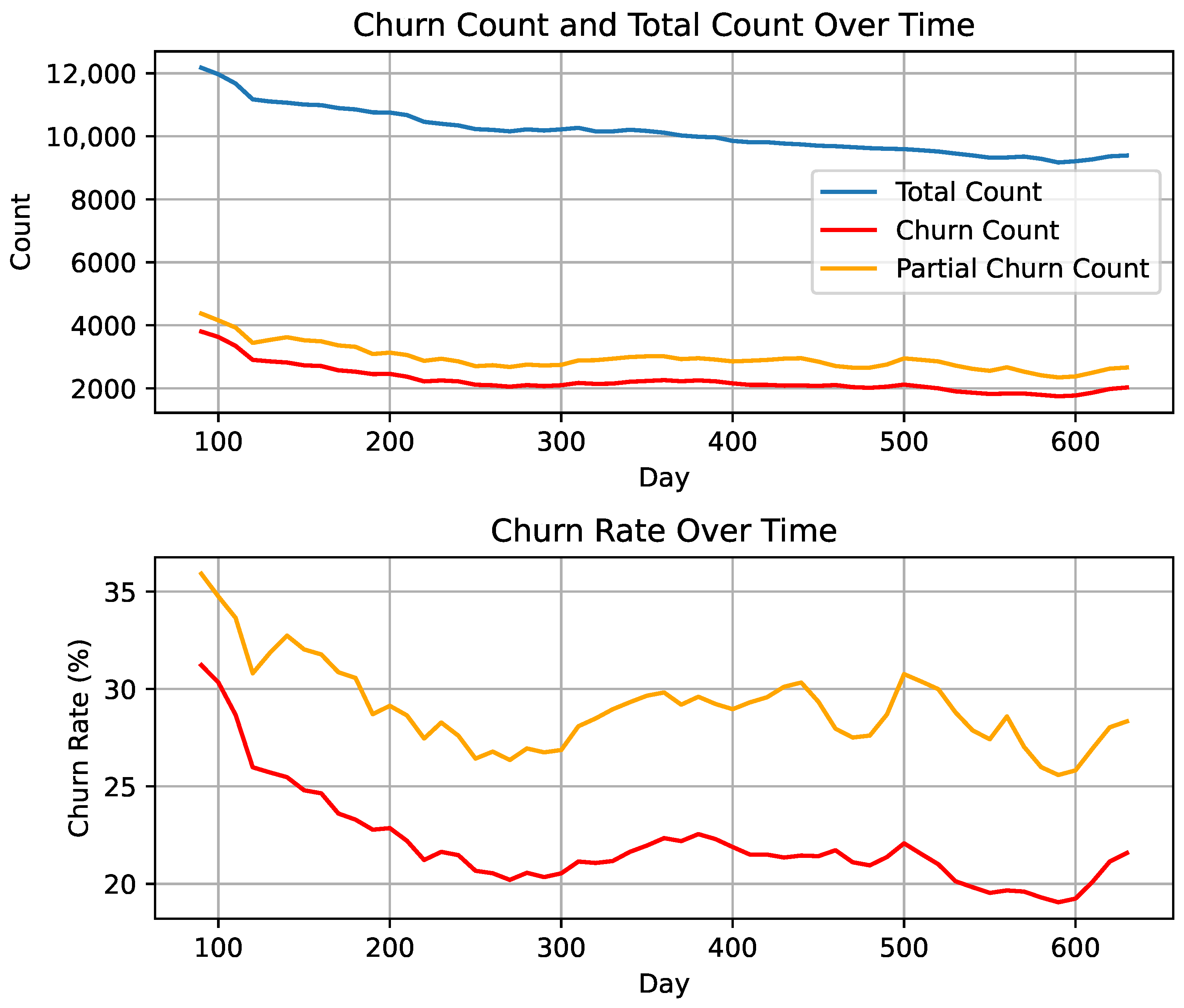
• The period of 90 days before the moment is used to extract features for the prediction;
• The period lasting up to 90 days after that moment is used to label data—40 days are used for partial churn labeling and 90 for full churn labeling.

We used Spark to create a big table and efficiently use it to establish daily aggregated parameters for every customer and each day of the raw data period. Next, we applied the sliding window approach to generate datasets. A window of 180 days is required to orient a dataset to a selected moment in time:

We illustrate our sliding window approach in Figure 2. The modeling moment is the moment we were referring to. Standard testing/learning refers to the period used to extract features for learning and testing. The simulation testing period is the interval used to extract features for prediction at the moment in time when, according to the model application simulation scenario, the labels are unknown; thus they are perfect test data, reflecting the real application scenario if the model was applied at that point in the past. Simulation labeling denotes the labels that are analogical to those used for training, i.e., the interval referred to in the figure as partial labeling. True labeling and standard labeling represent full churner labels for standard learning/testing features and simulation testing features, respectively. In other words:

• During its training, the model can “see” data derived from standard learning/testing and labels derived from partial labeling;
• Simulation testing/labeling intervals were used to create the ultimate test data that could simulate the model’s use in a real scenario;
• True/standard labeling intervals are used to provide alternative tests for those who want to keep track of churned customers who were labeled using the 90-day period, the so-called “full churners”.

2.2. Results Evaluation

To comprehensively assess the performance of our classification models and understand how different metrics relate to each other, we employed a methodological approach that involves transforming the metrics to address their bounded and non-linear nature, computing correlations, and constructing confidence intervals for the correlation coefficients.

2.2.1. Evaluation Metrics

We utilized three fundamental metrics to evaluate the performance of our models:

• Accuracy: The proportion of correct predictions among all predictions made. This is calculated as follows:

  $$\mathrm{Accuracy}={\displaystyle \frac{\mathrm{True}\mathrm{Positives}+\mathrm{True}\mathrm{Negatives}}{\mathrm{Total}\mathrm{Samples}}}$$

  (1)
  While accuracy provides a straightforward measure of performance, it can be misleading in datasets with imbalanced class distributions.
• F1 Score: The harmonic mean of precision and recall, providing a balance between the two. It is defined as follows:

  $$\mathrm{F}1\mathrm{Score}=2\times {\displaystyle \frac{\mathrm{Precision}\times \mathrm{Recall}}{\mathrm{Precision}+\mathrm{Recall}}}$$

  (2)
  The F1 score is particularly useful when the class distribution is uneven and when both false positives and false negatives are important.
• Area Under the ROC Curve (AUC): Measures the model’s ability to distinguish between classes by plotting the true positive rate against the false positive rate at various threshold settings. An AUC of 1 indicates perfect classification, while an AUC of 0.5 suggests no discriminative power.

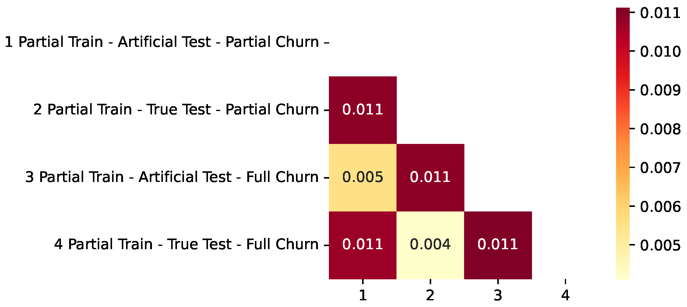
2.2.2. L2 Metric for Curve Difference Evaluation

In this research, we need to compare machine learning performance metrics; these metrics will be represented in the form of curves, with the horizontal axis representing different time windows. The L2 norm is widely used to evaluate the differences between curves as it provides a mathematically robust measure that captures the overall discrepancy across the entire domain. By integrating the squared differences in a point-wise manner, it highlights significant variations while smoothing out smaller ones. This approach aligns with the principles of functional analysis, where the L2 norm is often employed to quantify the energy-like differences between functions [43].

To evaluate the difference between two curves using the L2 norm, we replaced the pointwise differences with their squared counterparts and integrated over the domain of the curves:

$$A_{L2}=\sqrt{{\int }_{x_{\min }}^{x_{\max }}{\left(y_1\left(x\right)-y_2\left(x\right)\right)}^{2}dx}$$

(3)

In the experiments, we do not obtain the curve itself—we obtained a discrete set of points instead. These points were visually presented as piecewise linear graphs, and the integral was approximated numerically using the trapezoidal method. The trapezoidal method approximates the area under the curve by dividing it into trapezoids, summing their areas and thus providing an approximation of the integral. Applying this method to (3), we obtained the following:

$$A_{L2}\approx \sqrt{\sum _{i=1}^{n-1}{\displaystyle \frac{\Delta x_i}{2}}\left[{\left(y_{1i}-y_{2i}\right)}^2+{\left(y_{1(i+1)}-y_{2(i+1)}\right)}^2\right]}$$

(4)

where $\Delta x_i=x_{i+1}-x_i$ represents the interval width.

2.3. Hyperparameter Optimization

Choosing the proper parameter set for the machine learning method is a key task that affects all the results and conclusions of our research; thus, hyperparameter optimization must be applied to ensure the results are robust. The exception to this is the number of iterations, which is selected according to the validation set results—this also allows to use the early stopping mechanism, preventing optimization from unnecessary computation. We performed hyperparameter optimization for the CatBoost model using the Hyperopt library [44]. This library implements several algorithms for hyperparameter tuning, including random search and Bayesian optimization methods. We employed the Tree-structured Parzen Estimator (TPE) algorithm [45]. We used this algorithm because it provides an efficient, Bayesian-driven approach to hyperparameter optimization. Unlike grid or random search, TPE adaptively builds probability models for “good” versus “bad” hyperparameter configurations, helping it to focus on promising regions of the parameter space rather than randomly exploring every possibility. This often leads to faster convergence, especially in high-dimensional or complex search domains. TPE also handles both continuous and discrete parameters and can cope with non-convex, irregular loss surfaces, making it well-suited to the task of tuning CatBoost’s diverse hyperparameters in our experiments. In other words, it is an heuristic which can explore a much richer parameter space, often leading to improvements in the final results.

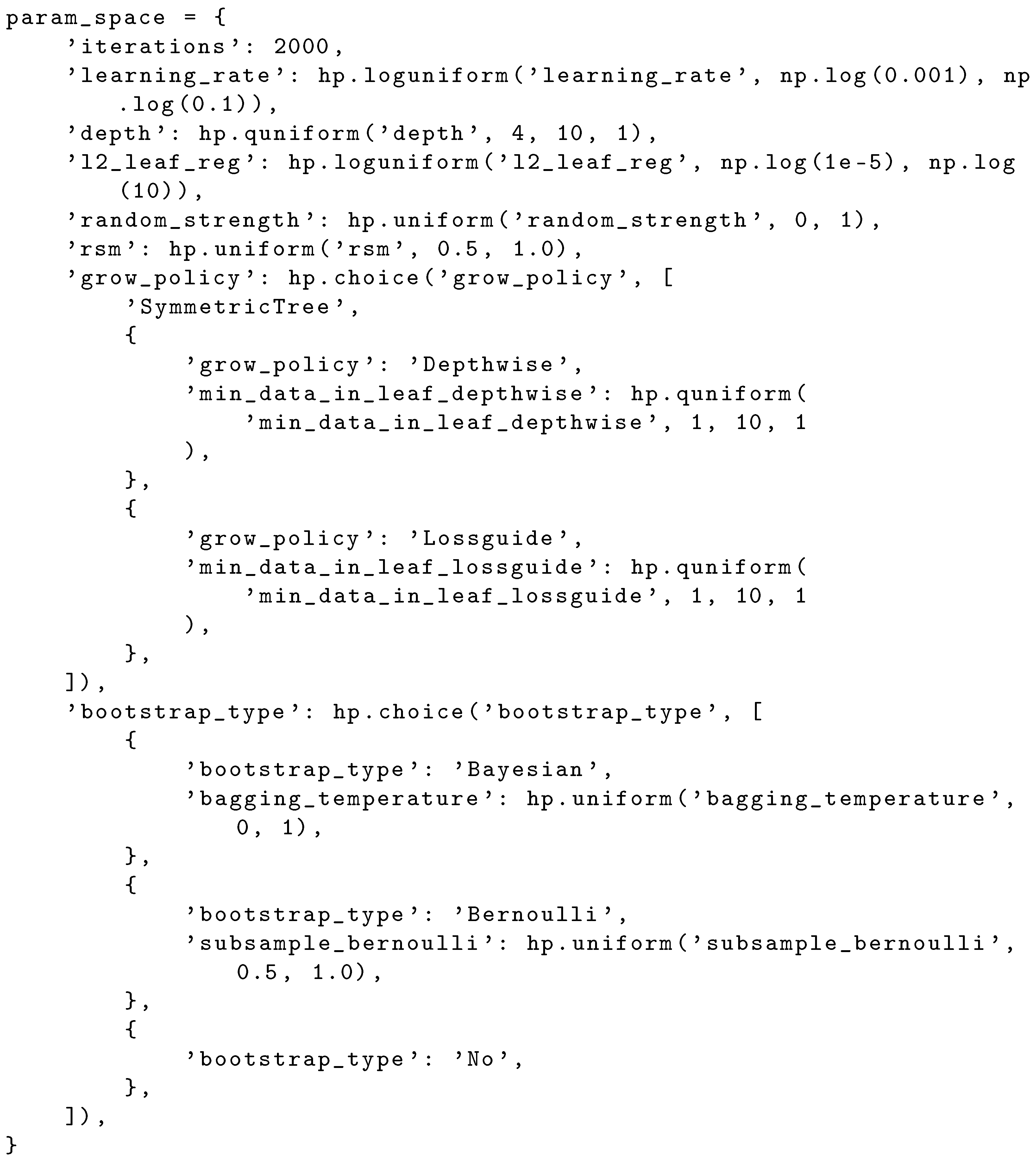
2.3.1. Parameter Space

The following hyperparameters and associated search distributions were defined (see Figure A4). Each hyperparameter was sampled from a specific probability distribution, ensuring a flexible search across a broad range of values:

• Iterations (parameter iterations): Fixed at 2000. A high iteration count was chosen, relying on early stopping in CatBoost to prevent overfitting.
• Learning rate (parameter learning_rate): Sampled from a log-uniform distribution over $[{10}^{-3},{10}^{-1}]$. Formally, if 

  $$x\sim \mathrm{Uniform}\left(log\left({10}^{-3}\right),log\left({10}^{-1}\right)\right),$$

  then

  $$\mathtt{learning}\_\mathtt{rate}=exp\left(x\right).$$
  This distribution is appropriate for the learning rates, which often span multiple orders of magnitude.
• Depth (parameter depth): Sampled from a quantized uniform distribution over $\{4,5,6,7,8,9,10\}$:

  $$\mathtt{depth}\sim \mathrm{QUniform}(4,10,1).$$
• L2 leaf regularization (parameter l2_leaf_reg): Sampled from a log-uniform distribution $[{10}^{-5},10]$. This controls the strength of the $L_2$ regularization in leaf values.
• Random strength (parameter random_strength) and random subspace method (rsm): Sampled from a uniform distribution over $[0,1]$ and $[0.5,1.0]$, respectively.
• Grow polic (parameter grow_policy): Chosen via parameter hp.choice among the following options:
  • SymmetricTree (no minimum data in leaf constraint);
  • Depthwise, requiring min_data_in_leaf_depthwise sampled from a quantized uniform distribution over $\{1,\dots ,10\}$;
  • Lossguide, requiring min_data_in_leaf_lossguide similarly sampled.
  This nested choice approach allowed us to conditionally sample a min_data_in_leaf parameter for the selected grow policy.
• Bootstrap type (parameter bootstrap_type): Chosen via hp.choice among the following options:
  • Bayesian, which also samples bagging_temperature from a uniform distribution $[0,1]$;
  • Bernoulli, which also samples subsample_bernoulli from a uniform distribution $[0.5,1.0]$;
  • No, which disables bootstrapping altogether.
  This conditional structure ensured that bagging_temperature or subsample were only relevant if the chosen bootstrap_type supported them.

In the CatBoost method there are four bootstrap options; however, we opted not to include Poisson bootstrap, due to its limitations (supported for GPU only) and to not use MVS because, according to the CatBoost documentation, “MVS may not be the best choice for regularization, since sampled examples and their weights are similar for close iterations” [46]. Thus, in our hyperparameter search, we focused on the most commonly used sampling methods—Bayesian and Bernoulli—preventing us from further complicating the search space without clear benefits for our particular data and objectives.

Figure A4 shows the precise Python definition in code.

2.3.2. Optimization Process

We employed a function for the Hyperopt library—this library uses the TPE algorithm, iterating over a maximum number of evaluations (specified as the parameter) to explore the parameter space. The TPE algorithm uses an iterative procedure, as follows:

• It initially randomly samples hyperparameter configurations;
• Then, it trains and evaluates a CatBoost classification model for each set of hyperparameters;
• It collects the performance results (F1 score, accuracy, etc.);
• It updates an internal model of “good” vs. “bad” hyperparameter densities;
• It proposes new configurations that are more likely to yield an improved performance.

Over multiple iterations, TPE effectively balances the exploration of diverse hyperparameter regions with the exploitation of promising configurations.

In our experiments, we recorded the negative of the F1 score as the loss to be minimized by TPE, thereby maximizing the F1. The best hyperparameter set was then retrained on the entire dataset (with appropriate oversampling) to produce the final CatBoost model. These and other hyperparameter optimization settings are summarized in

Table 3. Summary of hyperparameter optimization settings.

Optimization Setting	Value
Algorithm	Tree-structured Parzen Estimator (TPE)
Library	Hyperopt
Initial Random Evaluations	30 (via parameter n_startup_jobs)
Maximum Evaluations	300 (via parameter max_evals)
Cross-Validation Folds	5 (via parameter n_splits)
Objective Metric	Negative F1 score

.

3. Results

3.1. Hyperparameter Optimization

CatBoost is known to have a good initial hyperparameter set; however, as mentioned in Section 2.3, we used the Hyperopt library to optimize them on one of our datasets (the 90-day dataset). As a result, we achieved the parameters provided in

Table 4. Final set of hyperparameters obtained using Hyperopt on the 90-day dataset.

Parameter	Value
bootstrap_type	No
depth	5
grow_policy	SymmetricTree
l2_leaf_reg	0.357
learning_rate	0.058
random_strength	0.089
rsm	0.734
eval_metric	F1
early_stopping_rounds	50
verbose	100
iterations	121

.

Although the initial search space fixed the number of iterations at 2000 to allow for multiple boosting rounds, CatBoost often converges earlier when using early stopping. Specifically, after each hyperparameter configuration was evaluated via cross-validation, the median of the best (lowest-loss) iteration across folds was recorded. This value replaced the original iterations setting for the final model. Additionally, if the chosen bootstrap_type was No, parameters such as bagging_temperature or subsample were omitted, since they are not applicable under a no-bootstrap regime. Thus, the final hyperparameter dictionary included the actual number of boosting rounds used in practice and only parameters relevant to the selected bootstrap mode.

3.2. Dataset Properties

Here, we provide some important characteristics of our data. As  mentioned previously, in the context of ML we do not have a single dataset; instead, we slide windows and produce datasets for different time points.

In Figure 3, we present the amount of churned customers at different times points in the data.

As can be seen, the churn rate varies depending on the time window. As previously mentioned, we used the partial churn definition as the main label in our research. Note that the difference between full and partial churn is the number days of absence: 90 days for full churn and 40 for partial churn. We believe that 3 months is too long a period as processes are becoming more digitalized and faster; thus, we followed the observation in our previous study [24] of the hypothetical optimality of the partial churner definition and used it as the main way of labeling the data. However, from this definition it can be concluded that the full churner labels could form a subset of partial churn labels; if the client was absent for 90 days, they were necessarily absent for a 40-day period as well. The above is only true if the data are the same; in both cases, we filtered the data by dropping clients who were already churned according to the 40-day definition. As a consequence, if we used partial churn labels instead of full churn labels to train the model and predicted the full churn, it could be expected that this would increase recall and decrease precision, since it would increase both true and false positives. The hypothetical motivation for doing this could be to include more more recent data—however, in the context of our current research, the main reason for the use of partial churn labels instead of full churn labels is the fact that we used the partial churn definition as the main one. Thus, we will also provide results for the full churn definition for readers who still want to see how well the models can solving prediction problems with the full model definition.

From the churn rate, it is evident that the data are imbalanced; thus, we applied the random oversampling method to balance them. Note that this balancing was independently applied only to the learning part of every cross fold, completely removing any data leakage between the training and validation data and preserving the efficient early stopping during the model training.

3.3. ML Experiments’ Setup Cases

The central idea of our research is to keep in mind the concept drift problem, which, from a practical point of view, is closely related to the selection of appropriate test data. The test data must be from a future relating to that of the training data; to achieve this, we perfectly simulated the application of the model trained on past data, applying to the new, relevant data without labels. Thus, we followed the methodology described in Section 2: the dataset derived from the simulation testing/labeling window will be referred to as as the true testdataset; the dataset which was made from the standard testing/partial labeling window will be referred as the train dataset. More specifically, we measured six cases:

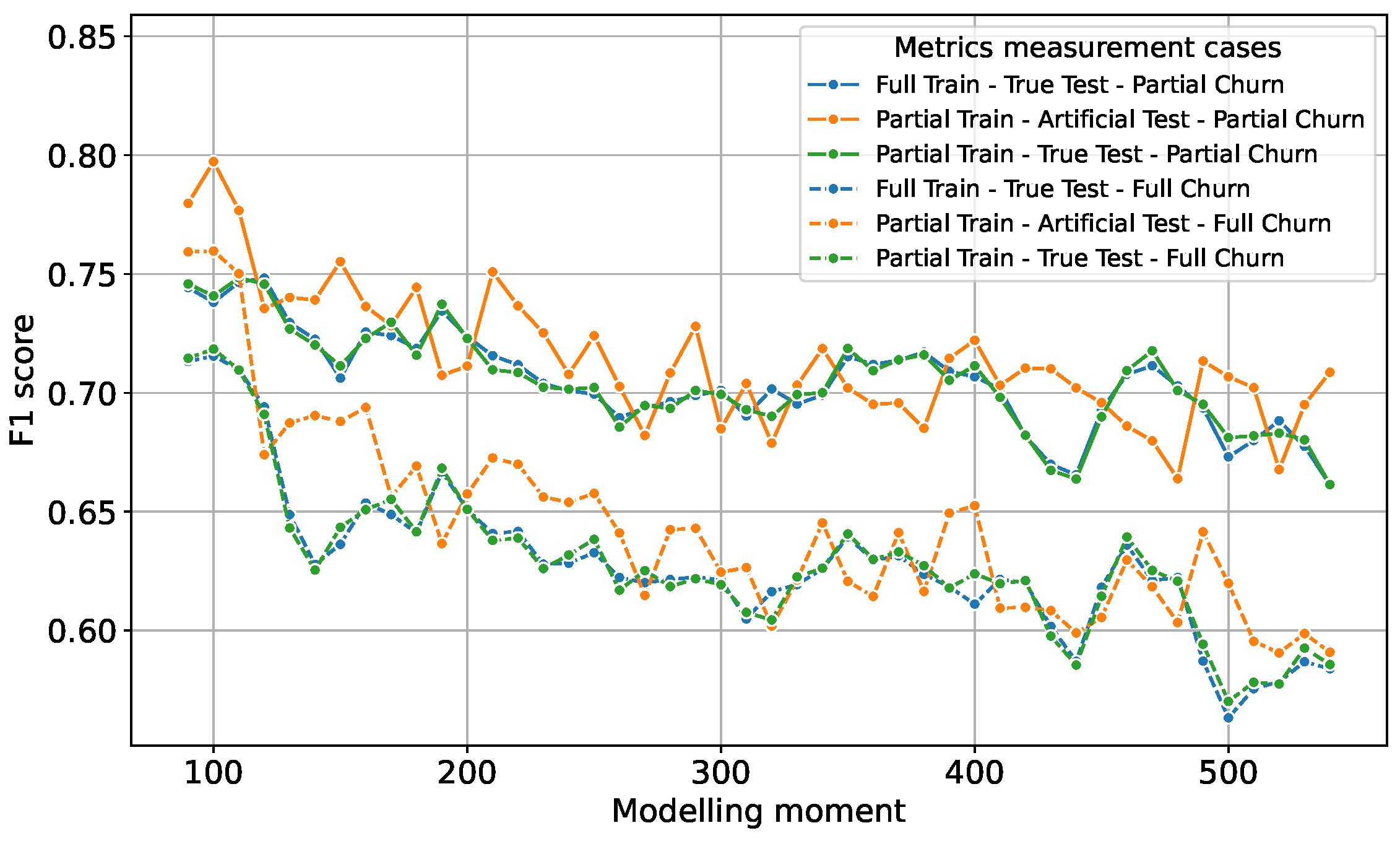
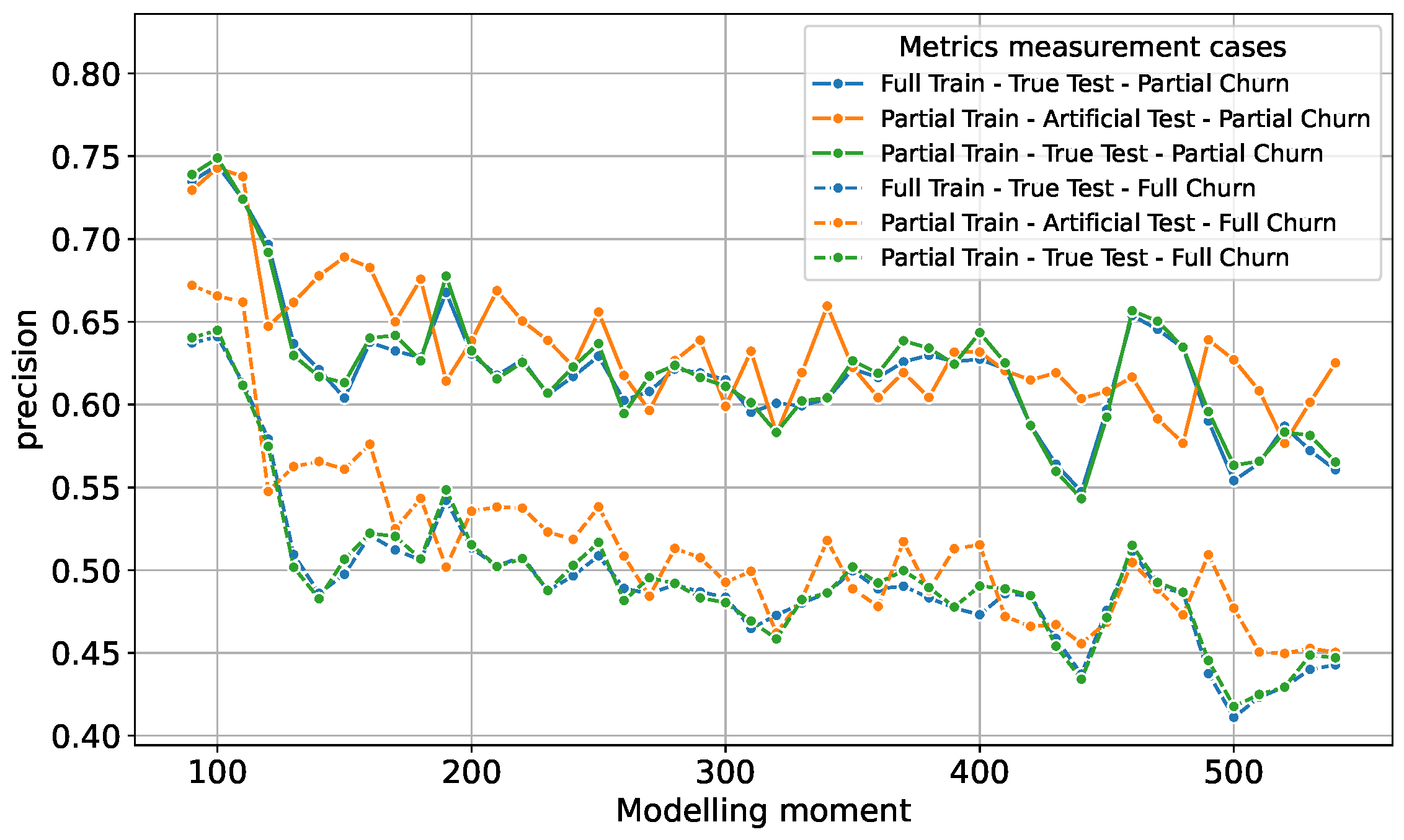
• An actual application case using the full train dataset for training and the true test dataset for testing, with metrics measuring partial churn prediction success. In the Figures, we refer to this as “Full Train–True Test–Partial Churn”.
• Same as the previous case, but with metrics measuring full churn prediction success. In the Figures, we refer to this as “Full Train–True Test–Full Churn”.
• An actual application case using the partial train dataset (80% sample) for training and true test dataset for testing. In the Figures, we refer to this as “Partial Train–True Test–Partial Churn”.
• Same as the previous case, but with metrics measuring full churn prediction success. In the Figures, we refer to this as “Partial Train–True Test–Full Churn”.
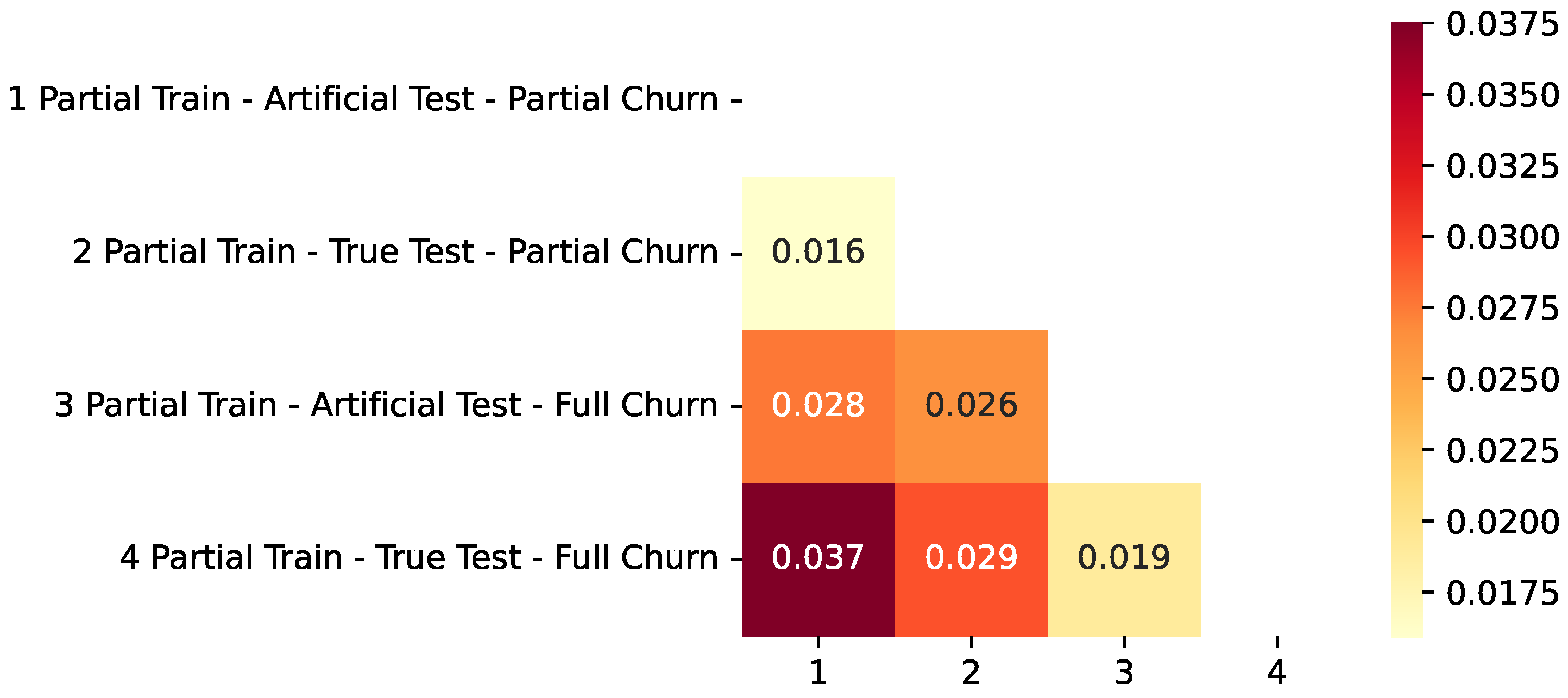
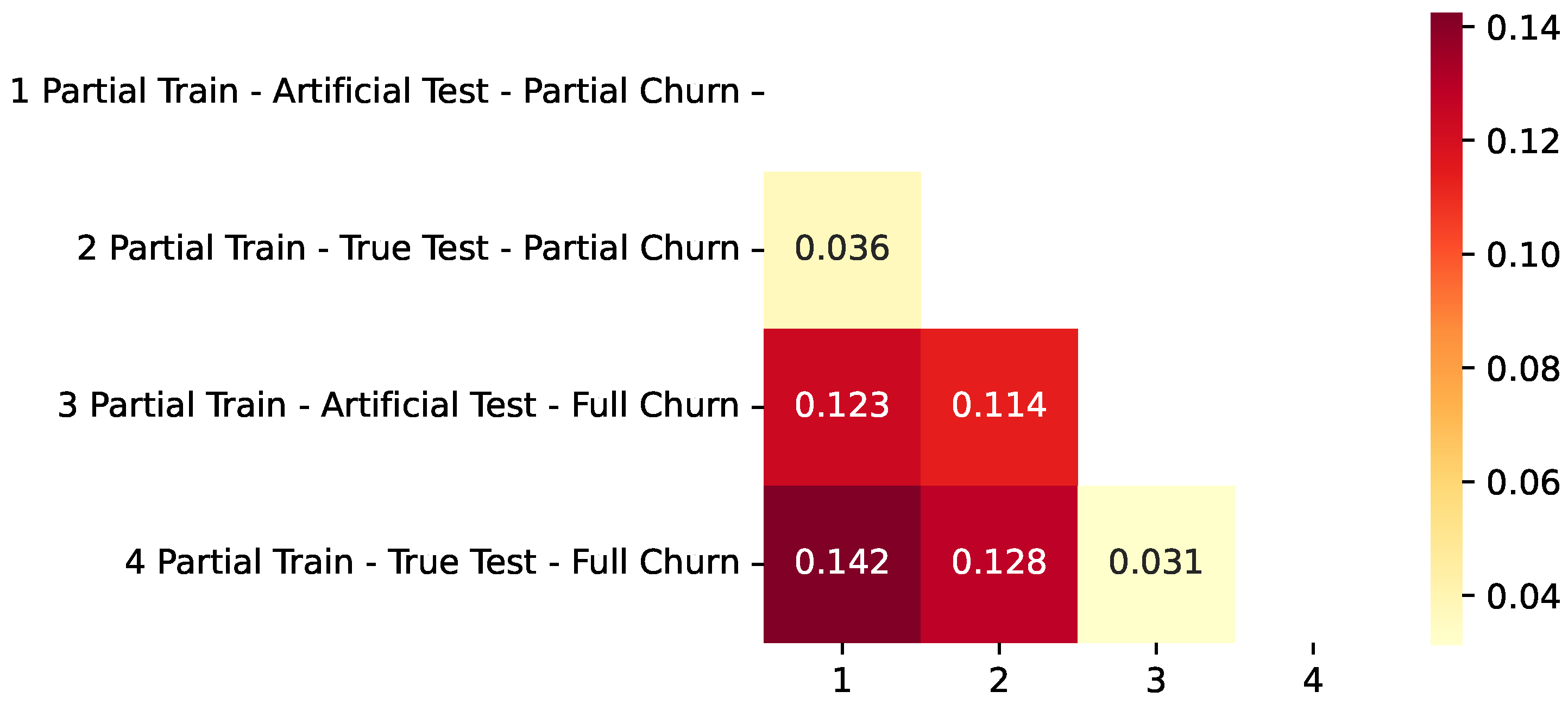
• A typical ML approach using a partial train dataset consisting of 80% of the initial data used for training, with the remaining 20% of the same dataset being used for testing—this testing is referred to as the artificial test. In the Figures, we refer to this as “Partial Train–Artificial Test–Partial Churn”.
• Same as the previous case, but with metrics measuring full churn prediction success. In the Figures, we refer to this as “Partial Train–Artificial Test–Full Churn”.

Cases 2, 4, and 6 evaluate the decrease in success when using a model trained using partial churner labels to predict the churner according to the full churn definition. Cases 3 and 4 are used as a clearer experiment to provide a comparison between the artificial test and true test, because otherwise the true test would have more data—we wanted to eliminate the positive effect of a larger amount of data on the success metrics in order to clarify the effect on concept drift. The comparison of cases 3 and 4 with cases 5 and 6 represents the effect of the drift shift—the true test and artificial test use data from different time windows, and the true test has a realistic delay of 40 days.

3.4. Analysis of the Results

In Figure 4, Figure 5 and Figure 6, the main metrics are provided for different cases, as discussed in Section 3.3. Note that the accuracy metric, in the context of our problem with imbalanced data, complements the main F1 score metric. Moreover, as can be seen in the figures, the overall patterns were similar in terms of F1 score and accuracy, although the F1 score shows more pronounced differences between partial and full churn scenarios. For a brief evaluation of the mode, we can refer to the “Full Train–True Test–Partial Churn” scenario as the main realistic practical scenario. The mean performance metrics across all time windows were 0.798 for accuracy, 0.704 for F1 score, and 0.8868 for AUC. Thus, we will omit further analysis of the accuracy metric.

As we can see from the metrics shown in Figure 4, Figure 5 and Figure 6, the full train and partial train graphs differ only slightly, suggesting that the reduction in 20% of the data used to label the artificial test data was not critical. Still, we were forced to compare them, because our main goal here was to compare true test and artificial test scenarios; thus, we maintained the same training sample size.

In this section, we present the results, focusing on the F1 score, area under the curve (AUC), recall, and precision over time. We studied these metrics to determine how the model performs under different training and testing situations, showing how concept drift affects the model and how the partial and full churn definitions are related.

Looking at the F1 results (Figure 4) for the “Partial Train–True Test–Partial Churn” and “Full Train–True Test–Partial Churn” cases shows that their curves look almost the same for most modeling periods, indicating that the smaller training set performs almost as well as the full dataset. Practically, this means that the same level of partial churn prediction accuracy can be maintained with fewer training examples, saving resources while preserving performance. Also, it means that we were able to compare true test and artificial test (when a part of the potential training data are reserved for testing purposes) scenarios using the same training sample size.

The AUC values (Figure 5) are always high for all settings, varying between 0.87 and 0.93. The AUC results for the “Full Train–True Test–Partial Churn” and “Partial Train–True Test–Partial Churn” hover at around 0.87–0.90. This range indicates that robust classification can be carried out using the partial churn definitions, though the results are slightly lower than the maximum AUC values seen in other scenarios. Nevertheless, the AUC differences between the full and partial churn scenarios were the smallest of all.

Figure 7 illustrates the recall for partial and full churn scenarios. The “Full Train-True Test-Full Churn” setup achieved recall values of around 0.9, indicating that the model effectively identifies full churners. The recall for partial churn scenarios is lower, even though full churners form a smaller subset of the partial churners. Note that the full churn problem obtained worse F1 performance (Figure 4) results compared to the partial churn problem despite the fact that the recall was better, i.e., using partial churn labels in training data for full churn prediction leads to more true positives being predicted at the cost of more false positives, which is reflected by the significantly lower precision score (Figure 8). Partial churner labels are formed from softer churn requirements compared to full churner labels, meaning that the signal indicating churn is stronger and true positives increase; this inevitably increases the recall.

However, Figure 8 shows that the full churn precision is lower, likely because the inclusion of borderline cases (users who are somewhat inactive but not definitively) leads to more false positives. A higher partial churn precision is a natural consequence of a model being trained on partially labeled data.

Some key observations that arise from these results are as follows: the fact that the partial churn predictions align with the full churn outcomes seems to suggest that full churners are a subset of partial churners. This relationship skews the performance metrics, especially the F1 scores and recall, which are lower for full-churn predictions, while the AUC remains relatively stable across full and partial churn scenarios. Additionally, the artificial test settings show slightly inflated metrics compared to the true tests, which further underlines the need for real application conditions for robust model evaluation. While the AUC stays rather constant across the full and partial churn scenarios, other metrics, such as F1 score and recall, are sensitive to temporal gaps.

Therefore, to further enhance the performance and reliability of the model, we recommend integrating dynamic model adaptation techniques for evolving customer behaviors. Investigation into cost-sensitive learning methods would probably allow for a better balance between precision and recall to be obtained, particularly in partial churn cases. Furthermore, additional experiments using smaller time windows or other datasets could validate these findings under different conditions.

In the “Partial Train–Artificial Test–Partial Churn” and “Full Train–True Test–Partial Churn” curves, the only difference was in the test data used. Figure 4 represents the most important metric F1 score. A similar pattern can be seen in terms of delay—the artificial test curve, in some instances, repeats the behavior of the true test curve with delay (we will try to measure this later). This could potentially indicate that the prediction success might depend more on the time windows on which it is tested than on the time windows on which it is trained.

Therefore, the results of our experiments led us to formulate the following two hypotheses:

Hypothesis 1.

The shift drift is less pronounced if we map the evaluations of predictions to the windows the predictions were applied to, rather than to the windows of the actual data on which the model was trained.

Hypothesis 2.

Full churn can be predicted using training data with partial churn labels without a significant drop in performance if the threshold value for prediction is modified.

As for the first hypotheses, we tried to investigate further. To take a closer look at the mentioned two curves, we considered an alternative view: instead of using the modeling moment on the horizontal axis, we used the time window the model used for testing. The result is represented by the dotted line in Figure 9.

The second hypothesis relies on the AUC metrics being almost identical for both churn definitions—the AUC is the only metric that does not depend on the threshold value for classification. This fact strongly supports this hypothesis, although we could not fully prove it.

Investigating the Proposed Hypotheses: Time-Window Shifts and Threshold Tuning

In order to find evidence supporting the first hypothesis, we first shifted the time window for true testing scenarios backward by 40 days. This can be seen as a change in the interpretation of the horizontal axis—now, it represents the time windows the model is being tested on, rather than the time window on which it was trained. Figure 9 shows both the original F1 scores for the “Partial Train–True Test–Partial Churn” and “Partial Train–Artificial Test–Partial Churn” scenarios and the shifted view of the first one (dotted line). Examining the three curves—’Partial Train–True Test–Partial Churn”, “Partial Train–Artificial Test–Partial Churn”, and “Partial Train–Artificial Test–Partial Churn (Shifted -40)”—we can observe that shifting the testing moments reduces the difference between the curves, as measured by Equation (4). Specifically, the difference between the curves without the shift was 0.025, while with a 40-day shift, this difference decreased to 0.0143. This supports Hypothesis 1, showing that mapping evaluations to the testing time windows reduces the impact of shift drift. Furthermore, this shift partly supports Hypothesis 2, as the smaller difference between the curves indicates that partial churn labels can be effectively used to predict full churn if the prediction threshold is properly adjusted.

The differences in AUC and F1 scores, measured using the L2 norm (as described in Section 2.2.2), were visualized through the heatmaps in Figure 10 and Figure 11, and reflect the variations observed in Figure 4 and Figure 5. The AUC showed minimal differences (range: 0.0041–0.0111), indicating that it remains largely unaffected by scenario variations. In contrast, the F1 score exhibited more significant variation (range: 0.025–0.0923), particularly between the full and partial churn scenarios, due to a sharp drop in the F1 scores for full churn predictions. These minimal AUC differences between the full and partial churn scenarios support Hypothesis 2, suggesting that partial churn labels can effectively approximate full churn predictions without significant performance loss, particularly when the AUC is the preferred metric. Meanwhile, the higher variability in F1 scores across scenarios indicates that the F1 is more sensitive to changes in classification results, as it combines both precision and recall.

Heatmaps for other metrics, including accuracy (range: 0.0159–0.0375), recall (range: 0.0237–0.0549), and precision (range: 0.0314–0.1424), are presented in Appendix A Figure A1, Figure A2 and Figure A3. Precision exhibited the highest variation, suggesting that the balance between true and false positive predictions is highly dependent on scenario and its specific factors. The additional metrics in Appendix A further highlight these trends, with accuracy and recall showing moderate robustness, while the heightened sensitivity of precision emphasizes the importance of careful threshold calibration.

In summary, the results underscore the critical role of metric selection in analyzing model performance under drift, with the AUC and F1 score providing the most significant evidence to validate the hypotheses.

Next, we further investigate the possibility of exploiting the specificity of the difference between full and partial churn scenarios, where the difference between these scenarios is small when using the decision threshold-independent metric of AUC and large when using other metrics, especially the F1 score. To investigate whether we can improve the F1 score, we deployed a new experimenta; setup with the following properties:

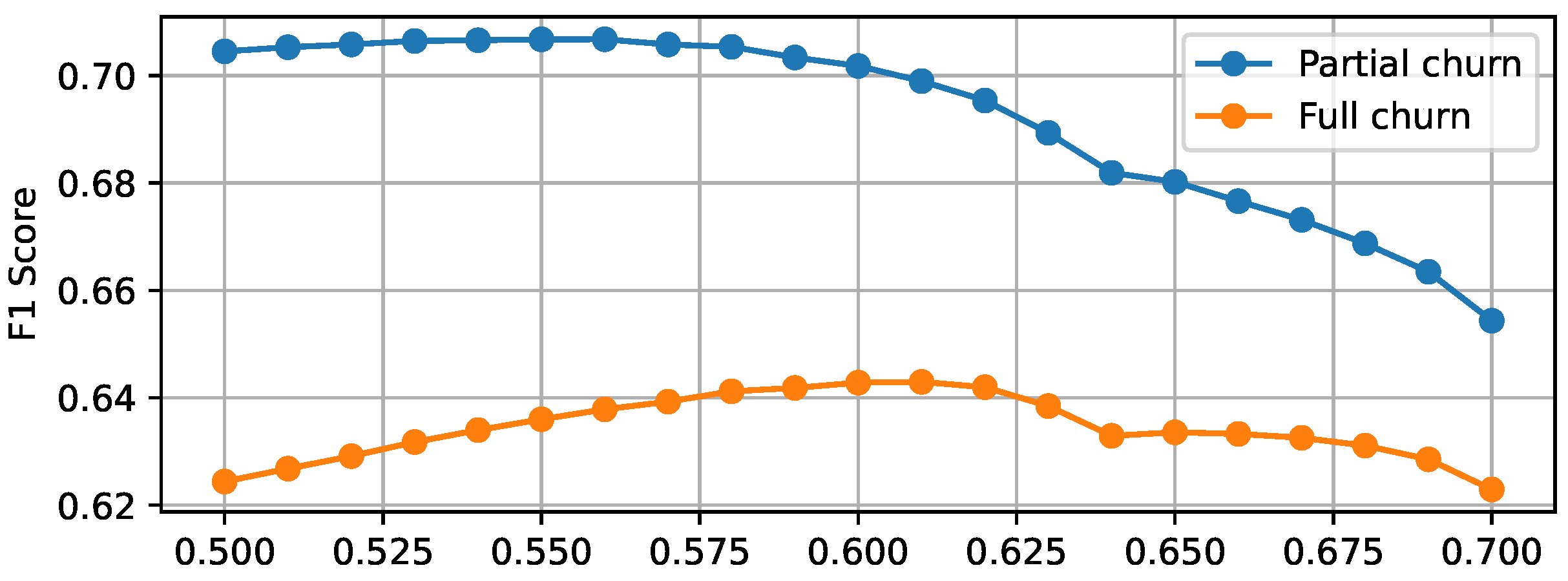
• We modified the original Catboost model by selecting a custom decision threshold, varying it from 0.5 to 0.7 with a step of 0.01.
• For clarity, we analyzed two scenarios that obtained the richest results from a practical point of view—both full train and true test scenarios, with different labels of partial and full churn, respectively.
• At each step, we evaluated the performance by averaging the F1 score metric over all time windows.
• Finally, we selected the decision threshold that obtained the best results and investigated it more closely.

The outcome of the first three points that were mentioned is provided in Figure 12. We can see that the full churn scenario performed best when the threshold value was around 0.6. The partial churn scenario started to perform worse—this is an expected result because the model was trained using partial churn labels. In short, there are two potential reasons that the full churn scenario might perform worse than the partial churn scenario:

• As previously mentioned, the model is trained to solve different tasks than it was tested on; although the difference is small, these differences lead to the unique effect of an indirect connection between tasks being observed.
• The complexities of the partial and full churn problems might be different, and the latter might be harder to predict. However, this specific question is beyond the scope of the current research, because it would require double the amount of computations without clear practical usefulness in the context of the current article.

We will ignore the slight improvement obtained when using partial churn with a threshold above 0.5, as it is insignificant and could be a natural result of nonlinearity of the model and the fact that we averaged the values over the time windows. As for the full churn scenario, the F1 score increased from 0.624 with threshold value 0.5 to 0.643 with threshold value 0.61.

Next, in Figure 13 we present the F1 score values for different modeling moments before and after the correction of threshold value. As can be observed, in the majority of cases, the correction improved the results; however, an anomaly with a single but significant drop of a single curve point can be observed. In order to analyze this result, we present the values for all confusion matrices as graphs in the Appendix. In Figure 14, it can be clearly observed that some spikes appear in the separate false/true negative/positive values. The expected result of the signals used to make decision being weakened (as a result of the higher threshold value) is due to the decrease in positive predictions and increase in negative predictions (both true and false ones). Thus, the F1 score improvement is due to the increase in true negative values and decrease in false positive values. The non-smooth spiky behavior of the false/true negative/positive values obtained for some custom values suggests that such an approach may be unreliable in practical applications. However, it is also evidence that the use of a stronger signal for churn prediction can improve the performance of the model, solving the full churn prediction problem. Thus, instead of engineering a modified custom decision threshold, assigning increased weights to the churn class could be a preferred approach, although it is beyond the scope of the current research. Future research might consider such a possibility.

4. Discussion

This paper presents a new methodology for churn prediction, using a unique temporal dataset and a sliding-window approach that creates multiple training and testing sets for different time windows. By structuring the data in this way, we aimed to simulate how models react to new information over time in a real-world setting. A summary of our main findings is provided below:

4.1. Model Evaluation

The performance metrics vary over time; however, for a brief evaluation, we can refer to the mean (across all time windows) performance metrics for the main realistic practical scenario: 0.798 for accuracy, 0.704 for F1 score, and 0.8868 for AUC. Although it is important to note that these results can vary a lot depending on the specifics of the data—for example, in other research, where different real data were used [47], the author achieved an F1 score of 0.989, which is well above the values achieved in other research using similar methods. Therefore, these values are only valid reference values in our research context. Therefore, the results cannot be considered comparable to those obtained by other authors using different data.

4.2. Model Relevance with Different Shifting Test Intervals

Our experiments suggest that the CatBoost model remains relevant even when trained on older data, indicating a certain resilience against concept drift in the sense that the model does not simply “expire” after a time gap. However, we also observe that the model performance varied across different testing windows: when the same model was applied to data from different future intervals, the predictive metrics would rise or fall. The primary reason for this was not a loss of validity in the training data; rather, the data to which the model was applied possessed changing characteristics over time. In other words, while the model does not become obsolete, its efficiency can vary based on when exactly we evaluate or deploy it. Such variations shows the importance of future-based testing scenarios (as opposed to artificial splits) to capture more realistic performance estimates. Although our study found only moderate differences, in more volatile environments these shifts could be larger, underscoring the need for periodic checks or incremental updates to maintain peak performance in real-world churn prediction.

4.3. Transfer Learning Without Extra Labels

One especially notable finding is that a model trained to predict partial churn (40-day inactivity) can also detect full churn (90-day inactivity) by simply adjusting its decision threshold. This means that organizations do not have to wait the full 90 days to label their training data; 40-day labels already capture enough churn-related information to be applied to 90-day churn predictions. Thus, a single model can cover both situations without a separate round of training being required for the longer inactivity labels, providing a practical example of transfer learning in churn prediction.

4.4. Unique Temporal Dataset and Practical Takeaways

Our dataset spans daily aggregated user metrics over 720 days for several thousand users. Rather than using just one training/testing split, we moved a 180-day window over time to produce multiple datasets. This design has the following advantages:

• It matches real-world cases where the training data always come before the data on which the model will be tested.
• It reveals certain drift patterns—CatBoost is relatively stable, yet its performance changes slightly with when future data are collected.
• It confirms that an 80% split for training can, in some cases, match the performance of a full training dataset.

4.5. Conceptual and Business-Level Implications

From a practical viewpoint, it is important to evaluate churn models on genuine future data. Reserving part of the same time period for testing can lead to overoptimistic performance measures. Although our dataset did not show extreme drift, we observed a significant differences between the ”artificial test” and ”true test” test sets, demonstrating that time-separated testing is crucial to see how well the model really performs under future conditions.

5. Conclusions

Overall, our study makes the following contributions to the research:

• It proposes a time-based testing methodology for telecommunication churn data, showing how models behave under realistic delays.
• It demonstrates that partial-churn labels can serve as a good substitute for full-churn labeling, saving weeks of waiting time without losing much predictive power.
• It confirms that CatBoost remained reasonably robust in our investigated time windows, though drift could become larger in rapidly changing environments, requiring ongoing checks or updates.

Threshold Choices and Potential Extensions. We found evidence that using a higher threshold can improve the performance of the full-churn prediction task. Instead of simply tuning thresholds, one might also consider assigning higher weights to the churn class during the training process. Although such strategies lie beyond the scope of this work, our results suggest they are promising directions. Future research could explore these techniques—along with dynamic threshold tuning, online learning, and cost-sensitive training—to see how well they reduce the impact of concept drift, particularly in more volatile markets or over longer time spans.

References

1. Vafeiadis, T.; Diamantaras, K.I.; Sarigiannidis, G.; Chatzisavvas, K.C. A comparison of machine learning techniques for customer churn prediction. Simul. Model. Pract. Theory 2015, 55, 1–9. [Google Scholar] [CrossRef]
2. Höppner, S.; Stripling, E.; Baesens, B.; Broucke, S.v.; Verdonck, T. Profit driven decision trees for churn prediction. Eur. J. Oper. Res. 2020, 284, 920–933. [Google Scholar] [CrossRef]
3. Toor, A.A.; Usman, M. Adaptive telecom churn prediction for concept-sensitive imbalance data streams. J. Supercomput. 2022, 78, 3746–3774. [Google Scholar] [CrossRef]
4. Alboukaey, N.; Joukhadar, A.; Ghneim, N. Dynamic behavior based churn prediction in mobile telecom. Expert Syst. Appl. 2020, 162, 113779. [Google Scholar] [CrossRef]
5. Gama, J.; Žliobaitė, I.; Bifet, A.; Pechenizkiy, M.; Bouchachia, A. A survey on concept drift adaptation. ACM Comput. Surv. (CSUR) 2014, 46, 44. [Google Scholar] [CrossRef]
6. Zhu, B.; Baesens, B.; vanden Broucke, S.K.L.M. An empirical comparison of techniques for the class imbalance problem in churn prediction. Inf. Sci. 2017, 408, 84–99. [Google Scholar] [CrossRef]
7. Manzoor, A.; Qureshi, M.A.; Kidney, E.; Longo, L. A Review on Machine Learning Methods for Customer Churn Prediction and Recommendations for Business Practitioners. IEEE Access 2024, 12, 70434–70463. [Google Scholar] [CrossRef]
8. Priya, S.; Uthra, R.A. Ensemble framework for concept drift detection and class imbalance in data stream. Multimed. Tools Appl. 2024. [CrossRef]
9. Sudharsan, R.; Ganesh, E.N. A Swish RNN based customer churn prediction for the telecom industry with a novel feature selection strategy. Connect. Sci. 2022, 34, 1855–1876. [Google Scholar] [CrossRef]
10. Garimella, B.; Prasad, G.; Prasad, M. Churn prediction using optimized deep learning classifier on huge telecom data. J. Ambient Intell. Humaniz. Comput. 2023, 14, 2007–2028. [Google Scholar] [CrossRef]
11. Pustokhina, I.V.; Pustokhin, D.A.; Nguyen, P.T.; Elhoseny, M.; Shankar, K. Multi-objective rain optimization algorithm with WELM model for customer churn prediction in telecommunication sector. Complex Intell. Syst. 2023, 9, 3473–3485. [Google Scholar] [CrossRef]
12. Arshad, S.; Iqbal, K.; Naz, S.; Yasmin, S.; Rehman, Z. A Hybrid System for Customer Churn Prediction and Retention Analysis via Supervised Learning. CMC-Comput. Mater. Contin. 2022, 72, 4283–4301. [Google Scholar] [CrossRef]
13. Beeharry, Y.; Tsokizep Fokone, R. Hybrid approach using machine learning algorithms for customers’ churn prediction in the telecommunications industry. Concurr. Comput. Pract. Exp. 2022, 34, e6627. [Google Scholar] [CrossRef]
14. Bogaert, M.; Delaere, L. Ensemble Methods in Customer Churn Prediction: A Comparative Analysis of the State-of-the-Art. Mathematics 2023, 11, 1137. [Google Scholar] [CrossRef]
15. Liu, Y.; Fan, J.; Zhang, J.; Yin, X.; Song, Z. Research on telecom customer churn prediction based on ensemble learning. J. Intell. Inf. Syst. 2023, 60, 759–775. [Google Scholar] [CrossRef]
16. Zhu, B.; Qian, C.; vanden Broucke, S.; Xiao, J.; Li, Y. A bagging-based selective ensemble model for churn prediction on imbalanced data. Expert Syst. Appl. 2023, 227, 120223. [Google Scholar] [CrossRef]
17. Nguyen, N.; Duong, T.; Chau, T.; Nguyen, V.H.; Trinh, T.; Tran, D.; Ho, T. A Proposed Model for Card Fraud Detection Based on CatBoost and Deep Neural Network. IEEE Access 2022, 10, 96852–96861. [Google Scholar] [CrossRef]
18. Ibrahim, A.; Ridwan, R.; Muhammed, M.; Abdulaziz, R.; Saheed, G. Comparison of the CatBoost Classifier with other Machine Learning Methods. Int. J. Adv. Comput. Sci. Appl. 2020, 11, 738–748. [Google Scholar] [CrossRef]
19. Hancock, J.; Khoshgoftaar, T. CatBoost for big data: An interdisciplinary review. J. Big Data 2020, 7, 94. [Google Scholar] [CrossRef]
20. Amin, A.; Adnan, A.; Anwar, S. An adaptive learning approach for customer churn prediction in the telecommunication industry using evolutionary computation and Naive Bayes. Appl. Soft Comput. 2023, 137, 110103. [Google Scholar] [CrossRef]
21. Alves, P.; Filipe, R.; Malheiro, B. Telco customer top-ups: Stream-based multi-target regression. Expert Syst. 2023, 40, e13111. [Google Scholar] [CrossRef]
22. Liu, X.; Liu, H.; Zheng, K.; Liu, J.; Taleb, T.; Shiratori, N. AoI-Minimal Clustering, Transmission and Trajectory Co-Design for UAV-Assisted WPCNs. IEEE Trans. Veh. Technol. 2025, 74, 1035–1051. [Google Scholar] [CrossRef]
23. Mitrovic, S.; Baesens, B.; Lemahieu, W.; De Weerdt, J. tcc2vec: RFM-informed representation learning on call graphs for churn prediction. Inf. Sci. 2021, 557, 270–285. [Google Scholar] [CrossRef]
24. Bugajev, A.; Kriauzienė, R.; Vasilecas, O.; Chadyšas, V. The impact of churn labelling rules on churn prediction in telecommunications. Informatica 2022, 33, 247–277. [Google Scholar] [CrossRef]
25. Kabas, O.; Ercan, U.; Dinca, M.N. Prediction of Briquette Deformation Energy via Ensemble Learning Algorithms Using Physico-Mechanical Parameters. Appl. Sci. 2024, 14, 652. [Google Scholar] [CrossRef]
26. Saha, L.; Tripathy, H.; Gaber, T.; El-Gohary, H.; El-kenawy, E.S. Deep churn prediction method for telecommunication industry. Sustainability 2023, 15, 4543. [Google Scholar] [CrossRef]
27. Ortakci, Y.; Seker, H. Optimising customer retention: An AI-driven personalised pricing approach. Comput. Ind. Eng. 2024, 188, 109920. [Google Scholar] [CrossRef]
28. Corporation, I. Telco Customer Churn. 2024. Available online: https://www.kaggle.com/datasets/blastchar/telco-customer-churn (accessed on 19 July 2024).
29. BigML. Telco Customer Churn: IBM Dataset. Available online: https://bigml.com/dashboard/source/669a36983b5846df24c14c0c (accessed on 19 July 2024).
30. Teradata Center for Customer Relationship Management at Duke University. Telecom Churn (cell2cell). Available online: https://www.kaggle.com/datasets/jpacse/datasets-for-churn-telecom (accessed on 19 July 2024).
31. Telecom_Churn. Available online: https://www.kaggle.com/datasets/priyankanavgire/telecom-churn (accessed on 19 July 2024).
32. Customer Churn Prediction 2020. Available online: https://www.kaggle.com/c/customer-churn-prediction-2020/data (accessed on 26 July 2024).
33. Customer Churn. Available online: https://www.kaggle.com/datasets/barun2104/telecom-churn (accessed on 26 July 2024).
34. Telecom_ Customer. Available online: https://www.kaggle.com/datasets/abhinav89/telecom-customer (accessed on 1 August 2024).
35. South Asian Churn Dataset. Available online: https://www.kaggle.com/datasets/mahreen/sato2015/data (accessed on 30 August 2024).
36. Orange Telecom Dataset. Available online: https://www.kdd.org/kdd-cup/view/kdd-cup-2009 (accessed on 30 August 2024).
37. Al-Shourbaji, I.; Helian, N.; Sun, Y.; Alshathri, S.; Abd Elaziz, M. Boosting Ant Colony Optimization with Reptile Search Algorithm for Churn Prediction. Mathematics 2022, 10, 1031. [Google Scholar] [CrossRef]
38. Tavassoli, S.; Koosha, H. Hybrid ensemble learning approaches to customer churn prediction. Kybernetes 2022, 51, 1062–1088. [Google Scholar] [CrossRef]
39. Kozak, J.; Kania, K.; Juszczuk, P.; Mitręga, M. Swarm intelligence goal-oriented approach to data-driven innovation in customer churn management. Int. J. Inf. Manag. 2021, 60, 102357. [Google Scholar] [CrossRef]
40. Mirza, O.M.; Moses, G.J.; Rajender, R.; Lydia, E.L.; Kadry, S.; Me-Ead, C.; Thinnukool, O. Optimal Deep Canonically Correlated Autoencoder-Enabled Prediction Model for Customer Churn Prediction. CMC-Comput. Mater. Contin. 2022, 73, 3757–3769. [Google Scholar] [CrossRef]
41. Wu, S.; Yau, W.C.; Ong, T.S.; Chong, S.C. Integrated Churn Prediction and Customer Segmentation Framework for Telco Business. IEEE Access 2021, 9, 62118–62136. [Google Scholar] [CrossRef]
42. Adhikary, D.D.; Gupta, D. Applying over 100 classifiers for churn prediction in telecom companies. Multimed. Tools Appl. 2020, 80, 1–22. [Google Scholar] [CrossRef]
43. Adams, R.A.; Fournier, J.J. Sobolev Spaces; Elsevier: Amsterdam, The Netherlands, 2003. [Google Scholar]
44. Bergstra, J.; Yamins, D.; Cox, D. Making a science of model search: Hyperparameter optimization in hundreds of dimensions for vision architectures. In Proceedings of the International Conference on Machine Learning, PMLR, Atlanta, GA, USA, 16–21 June 2013; pp. 115–123. [Google Scholar]
45. Bergstra, J.; Bardenet, R.; Bengio, Y.; Kégl, B. Algorithms for hyper-parameter optimization. Adv. Neural Inf. Process. Syst. 2011, 24. [Google Scholar]
46. Bootstrap Options. Available online: https://catboost.ai/docs/en/concepts/algorithm-main-stages_bootstrap-options (accessed on 28 January 2025).
47. Przybyła-Kasperek, M.; Marfo, K.F.; Sulikowski, P. Multi-Layer Perceptron and Radial Basis Function Networks in Predictive Modeling of Churn for Mobile Telecommunications Based on Usage Patterns. Appl. Sci. 2024, 14, 9226. [Google Scholar] [CrossRef]
Figure 1. The number of articles by year obtained using the CatBoost method. This result was obtained from the Web Of Science platform with an advanced search query, “TS = (CatBoost) OR AK = (CatBoost)”.
Applsci 15 01599 g001
Figure 2. Simulation modeling. The red dotted line represents the moment in time that was simulated.
Applsci 15 01599 g002
Figure 3. Churn rate.
Applsci 15 01599 g003
Figure 4. F1 score.
Applsci 15 01599 g004
Figure 5. AUC (Area under curve).
Applsci 15 01599 g005
Figure 6. Accuracy.
Applsci 15 01599 g006
Figure 7. Recall.
Applsci 15 01599 g007
Figure 8. Precision.
Applsci 15 01599 g008
Figure 9. F1 score for different testing time windows vs. modeling moment time windows.
Applsci 15 01599 g009
Figure 10. F1 score differences using the L2 norm between scenarios.
Applsci 15 01599 g010
Figure 11. AUC differences using the L2 norm between scenarios.
Applsci 15 01599 g011
Figure 12. F1 performance with different model thresholds.
Applsci 15 01599 g012
Figure 13. F1 scores with the default and corrected thresholds.
Applsci 15 01599 g013
Figure 14. Confusion matrices with the default and corrected thresholds.
Applsci 15 01599 g014