Experimental Validation of Offset-Free Model-Based Predictive Control in Voltage Source Inverters for Grid Connected and Microgrids Applications

Abstract

This article presents the experimental validation of a model-based predictive control (MPC) strategy for the safe interconnection of voltage source inverters (VSI) with output LC filters for the grid connection of DC energy resources. The MPC is formulated as a quadratic programming (QP) problem and solved using the operator splitting quadratic programs (OSQP). The proposed approach incorporates integral action to achieve precise voltage magnitude reference tracking while accounting for modulated voltage limits and nominal current constraints within the control design. The effectiveness of the proposed strategy is validated through simulations conducted in MATLAB, demonstrating superior dynamic performance compared to the traditional hierarchical PI control. The implementation of the proposed MPC is experimentally verified on a VSI setup using the dSPACE MicroLabBox. The results confirm that the computational requirements are satisfied, establishing this approach as a practical alternative for modern power electronic systems. The proposed MPC for VSIs offers an effective approach to enforcing operational constraints, improving dynamic performance, and facilitating the robust integration of renewable energy sources in microgrids.

1. Introduction

Voltage source inverters (VSIs) are a common interface in modern power electronic systems, facilitating the conversion between direct-current (DC) and alternating-current (AC) domains [1,2]. These devices are widely used in various technological applications, such as advanced motor drive systems [3,4], renewable energy systems, and distributed energy resources (DERs) [5].

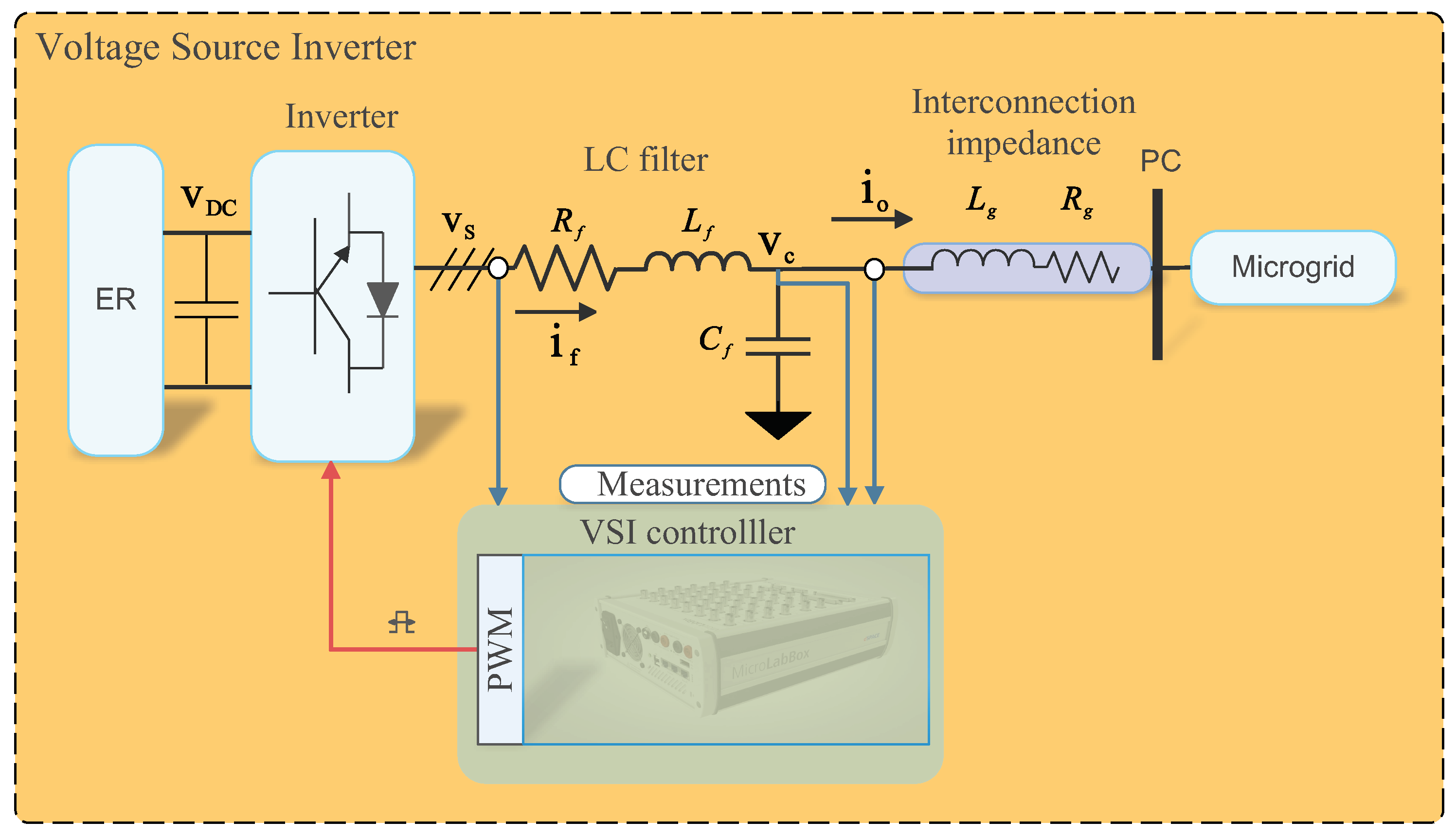
Figure 1 presents a generic representation of the VSI control system. The energy resource (ER) typically consists of sources such as photovoltaic panels (PV) [6], battery energy storage systems (BESS) [7], or wind energy systems (WES) [8]. The inverter converts the ER’s DC voltage into AC and is connected through an LC filter to attenuate high-frequency harmonics. An isolation transformer is used to connect to the point of coupling (PC), facilitating the connection to the microgrid or local loads. This system is equipped with sensors to measure the voltages and currents required for the VSI controller. The control objective of the VSI is to achieve reference tracking of the LC filter’s output voltage with robustness and low distortion. The control action is sent to a pulse-width modulation (PWM) to generate the inverter’s triggering pulses [9,10].

The voltage control of the LC filter requires advanced strategies compared to current control in grid-connected converters [9]. Typically, proportional-integral (PI) cascaded control strategies are employed [11,12]. These strategies have the advantage of imposing restrictions on the converter current by imposing limits on its reference; however, they result in limited dynamic performance [13]. Multiple-input multiple-output (MIMO) control strategies have been proposed [12] for VSI control. Nevertheless, these approaches often preserve the cascaded control structure. State feedback control with disturbance compensation has also been proposed [14], satisfying the dynamic performance objectives. However, this strategy does not allow for imposing the converter’s physical constraint. The control of VSIs can be formulated using Model Predictive Control (MPC) to achieve a dynamic performance consistent with MIMO optimal control when operational constraints are not violated. Furthermore, MPC offers the distinctive advantage of directly incorporating operational and physical constraints into the control design process [15], effectively overcoming the performance limitations of hierarchical control structures. This topic has gained significant attention in recent years, prompting researchers to propose various MPC strategies for VSIs [16,17,18]. In [16], an implicit MPC is proposed, using a custom active set method to solve the optimization problem. The estimated computational complexity of the algorithm is five times lower than explicit MPC formulations, but only for a prediction horizon of one, and only simulation results are presented. In [18], simulation results using MATLAB / Simulink show the use of finite control set model predictive control (FCS-MPC) with horizon one for voltage control of VSIs in a droop-controlled standalone AC microgrid. None of the two previous works incorporate integration for voltage regulation. In [19], an FCS-MPC strategy is proposed again with a prediction horizon of one, but with delay compensation, incorporating an observer that provides integration to the control. This mitigates the effects of uncertainties in voltage regulation. Experimental results obtained in a laboratory setup validate the proposal. However, tuning the bandwidth of an FCS-MPC controlled system is not possible; it has stringent requirements on sampling time and produces a spread switching harmonics spectra, which is undesirable.

In general, the MPC strategy can be formulated as a quadratic programming (QP) problem, minimizing a quadratic cost function subject to linear constraints [20,21]. Several solvers are available for QP problems, such as MOSEK [22], GUROBI [23], ECOS [24], and OSQP [25]. Proper selection of the QP solver is crucial to meet the time requirements for fast dynamic systems. In [25], the authors present a benchmark comparing OSQP with MOSEK, GUROBI, and ECOS. This work shows that the OSQP solver, based on the alternating direction method of multipliers (ADMM), has fast response times and reliable performance compared to other alternatives. Moreover, it is open-source and suitable for embedded implementations. Additionally, other implementations of ADMM have been extensively studied for power electronic systems applications [26,27,28].

This work introduces an MPC for the control of a voltage source inverter. The proposed algorithm is formulated based on dynamic performance criteria and incorporates integral action to mitigate unmodeled errors and system disturbances. The MPC is designed as a QP problem, where the predictive dynamic model is included as a linear equality constraint and physical and operational constraints are expressed as linear inequalities. MATLAB simulations demonstrate the superior performance of the proposed approach compared to conventional hierarchical PI control. The optimization problem is solved using the OSQP algorithm, achieving real-time execution with an average computation time of approximately $70\mathsf{\mu }\mathrm{s}$ using the MicroLabox controller of dSPACE, confirming its suitability for microgrid applications.

2. Materials and Methods

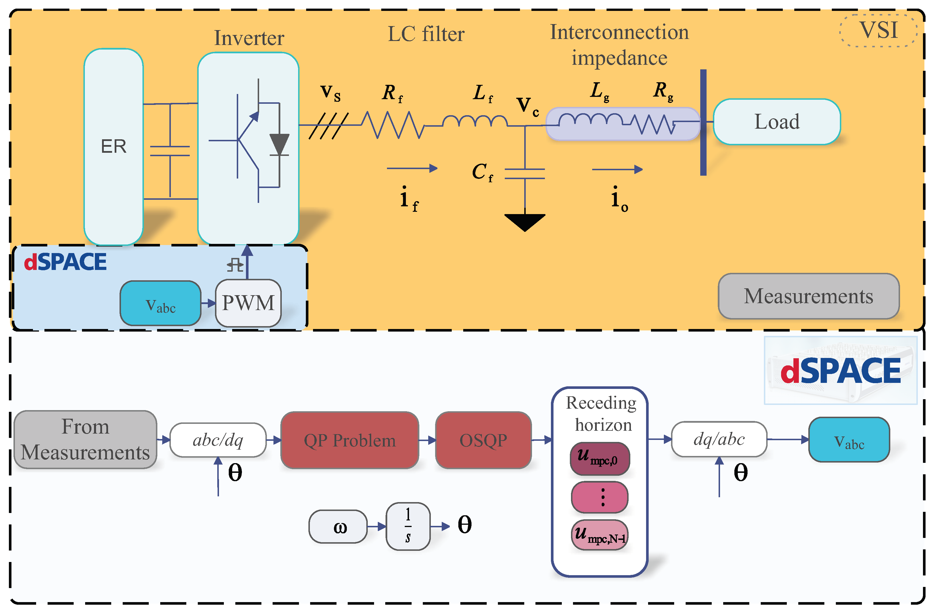
Figure 2 presents the schematic of the voltage source inverter connected to the grid and the voltage control system examined in this paper. To focus exclusively on voltage control, the grid interaction is excluded from this study, and the inverter is connected to a local resistive load. The controller processes measurements of the output voltage, filter current, and output current, converting them into the $dq$ reference frame. These $dq$ variables are subsequently used to formulate a quadratic programming (QP) problem. The optimal control problem is solved using the OSQP solver with a receding horizon approach. The resulting control actions are then transformed back into the $abc$ reference frame and applied using PWM modulation. The parameters of the laboratory experimental setup used in this study are summarized in

Table 1. Parameters of the system.

System Parameters	Value	Remark
$v_{\mathrm{dc}}$	$300\mathrm{V}$	DC Bus
$i_{\mathrm{n}}$	$10\mathrm{A}$	Nominal current
$L_{\mathrm{f}}$	$5\mathrm{mH}$	Filter inductance
$C_{\mathrm{f}}$	$12\mathsf{\mu }\mathrm{F}$	Filter capacitor
$R_{\mathrm{f}}$	$0.065\mathsf{\Omega }$	Filter resistance
$\omega$	$2\pi 50\mathrm{rad}/\mathrm{s}$	Nominal frequency
$T_{\mathrm{s}}$	$200\mathsf{\mu }\mathrm{s}$	Sampling time

.

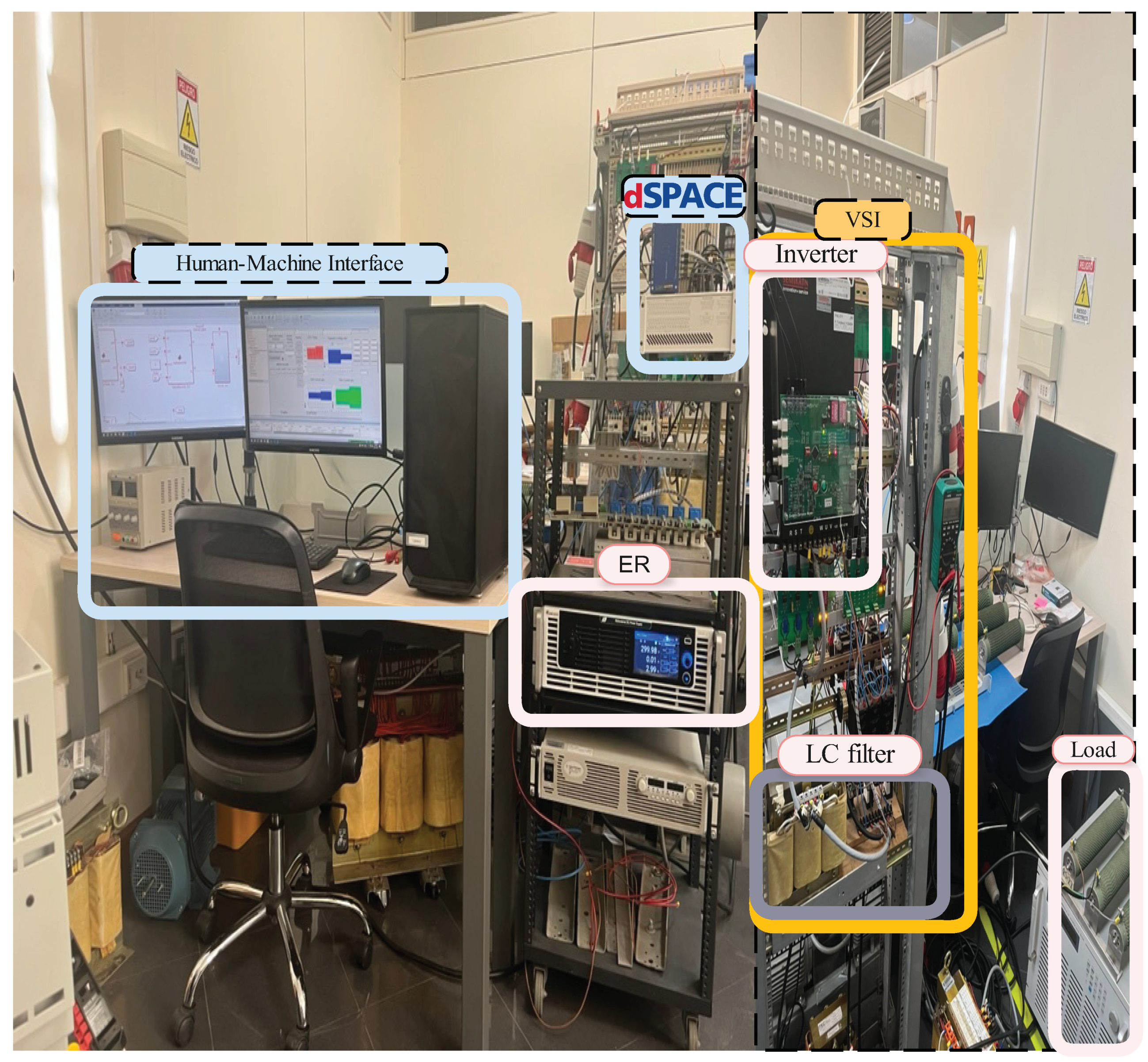
Figure 3 shows the experimental setup used to evaluate the proposed MPC control for the voltage source inverter (VSI). In this setup, the energy resource (ER) is emulated using a Chroma 62060 regenerative DC power supply, which provides the necessary DC-link voltage for a Semikron three-phase inverter. An LC filter is implemented to attenuate high-frequency harmonics in the three-phase voltage (${\mathbf{v}}_{\mathrm{s}}$) and produce a smooth output capacitor voltage (${\mathbf{v}}_{\mathrm{c}}$). The VSI configuration includes an output transformer, modeled as an unknown series impedance for control purposes, that is connected to a star-connected resistor bank with a resistance of 47 $\mathsf{\Omega }$ per phase. Furthermore, a star-connected resistor bank of 23 $\mathsf{\Omega }$ is connected in parallel through a breaker, allowing the introduction of a load disturbance into the system. Filter currents, output voltages, and output currents are measured using custom-designed sensor boards. The dSPACE MicroLabBox acquires these measurements via its analog-to-digital (ADC) channels for control purposes.

3. Voltage Source Inverter Model

This section provides a brief description of the dynamic model of the VSI and the filter used in the experimental setup for this study. The dynamic model of the filter is expressed in the $dq$ synchronous reference frame by applying the Clarke and Park transformations (1) and (2):

$$\begin{array}{c}\hfill \left[\begin{array}{c}{v}_{\mathrm{c}\alpha }\\ v_{\mathrm{c}\beta }\end{array}\right]=\left[\begin{array}{ccc}{\displaystyle \frac{2}{3}}& -{\displaystyle \frac{1}{3}}& -{\displaystyle \frac{1}{3}}\\ 0& {\displaystyle \frac{1}{\sqrt{3}}}& -{\displaystyle \frac{1}{\sqrt{3}}}\end{array}\right]\left[\begin{array}{c}{v}_{\mathrm{c}\mathrm{a}}\\ v_{\mathrm{c}\mathrm{b}}\\ v_{\mathrm{c}\mathrm{c}}\end{array}\right],\end{array}$$

(1)

$$\begin{array}{c}\hfill \left[\begin{array}{c}{v}_{\mathrm{c}\mathrm{d}}\\ v_{\mathrm{c}\mathrm{q}}\end{array}\right]=\left[\begin{array}{cc}cos\theta & sin\theta \\ -sin\theta & cos\theta \end{array}\right]\left[\begin{array}{c}{v}_{\mathrm{c}\alpha }\\ v_{\mathrm{c}\beta }\end{array}\right].\end{array}$$

(2)

In (2), the angle $\theta$ is determined by integrating the reference frequency of capacitor voltage ($\theta =\int \omega dt$). The resulting dynamic model of the LC filter is described by the following equations [14,26]:

$$\begin{array}{c}\hfill \begin{array}{cc}\hfill L_{\mathrm{f}}{\displaystyle \frac{d{\mathbf{i}}_{\mathrm{f}}}{dt}}& =-R_{\mathrm{f}}{\mathbf{i}}_{\mathrm{f}}-j\omega L_{\mathrm{f}}{\mathbf{i}}_{\mathrm{f}}-{\mathbf{v}}_{\mathrm{c}}+{\mathbf{v}}_{\mathrm{s}},\hfill \\ \hfill C_{\mathrm{f}}{\displaystyle \frac{d{\mathbf{v}}_{\mathrm{c}}}{dt}}& ={\mathbf{i}}_{\mathrm{f}}-j\omega C_{\mathrm{f}}{\mathbf{v}}_{\mathrm{c}}-{\mathbf{i}}_{\mathrm{o}}.\hfill \end{array}\end{array}$$

(3)

where $\{L_{\mathrm{f}},R_{\mathrm{f}},C_{\mathrm{f}}\}$ are the LC filter parameters, ${\mathbf{i}}_{\mathrm{f}}={\left[i_{\mathrm{fd}}{i}_{\mathrm{fq}}\right]}^{\top }$ is the current vector at the inductor, ${\mathbf{v}}_{\mathrm{s}}={\left[v_{\mathrm{sd}}{v}_{\mathrm{sq}}\right]}^{\top }$ is the inverter modulated voltage vector, and ${\mathbf{i}}_{\mathrm{o}}={\left[i_{\mathrm{od}}{i}_{\mathrm{oq}}\right]}^{\top }$ is the output current. Equation (3) can be expressed in a continuous state-space model, where the voltage and current are separated into their real and imaginary components:

$$\begin{array}{c}\hfill \begin{array}{cc}\hfill {\displaystyle \frac{d}{dt}}\left[\begin{array}{c}{i}_{\mathrm{fd}}\\ i_{\mathrm{fq}}\\ v_{\mathrm{cd}}\\ v_{\mathrm{cq}}\end{array}\right]& =\left[\begin{array}{cccc}-{\displaystyle \frac{R_{\mathrm{f}}}{L_{\mathrm{f}}}}& \omega & -{\displaystyle \frac{1}{L_{\mathrm{f}}}}& 0\\ -\omega & -{\displaystyle \frac{R_{\mathrm{f}}}{L_{\mathrm{f}}}}& 0& -{\displaystyle \frac{1}{L_{\mathrm{f}}}}\\ {\displaystyle \frac{1}{C_{\mathrm{f}}}}& 0& 0& \omega \\ 0& {\displaystyle \frac{1}{C_{\mathrm{f}}}}& -\omega & 0\end{array}\right]\left[\begin{array}{c}{i}_{\mathrm{fd}}\\ i_{\mathrm{fq}}\\ v_{\mathrm{cd}}\\ v_{\mathrm{cq}}\end{array}\right]+\left[\begin{array}{cc}{\displaystyle \frac{1}{L_{\mathrm{f}}}}& 0\\ 0& {\displaystyle \frac{1}{L_{\mathrm{f}}}}\\ 0& 0\\ 0& 0\end{array}\right]{\mathbf{v}}_{\mathrm{s}}+\left[\begin{array}{cc}0& 0\\ 0& 0\\ -{\displaystyle \frac{1}{C_{\mathrm{f}}}}& 0\\ 0& -{\displaystyle \frac{1}{C_{\mathrm{f}}}}\end{array}\right]{\mathbf{i}}_{\mathrm{o}},\hfill \\ \hfill \mathbf{y}& =\left[\begin{array}{cc}{\mathbf{0}}_{2\times 2}& {\mathbb{I}}_{2\times 2}\end{array}\right]{\left[\begin{array}{cccc}{i}_{\mathrm{fd}}& i_{\mathrm{fq}}& v_{\mathrm{cd}}& v_{\mathrm{cq}}\end{array}\right]}^{\top }.\hfill \end{array}\end{array}$$

(4)

The system of Equation (4) can be expressed in its compact form as follows:

$$\begin{array}{c}\hfill \begin{array}{cc}\hfill \dot{\mathbf{x}}& =\mathbf{A}\mathbf{x}+\mathbf{B}\mathbf{u}+{\mathbf{B}}_{\mathrm{p}}{\mathbf{i}}_{\mathrm{o}},\hfill \\ \hfill \mathbf{y}& =\mathbf{C}\mathbf{x}.\hfill \end{array}\end{array}$$

(5)

From (5), the system’s discrete state-space representation is derived using a sampling period $T_{\mathrm{s}}$, as outlined in [14,26]:

$$\begin{array}{c}\hfill \begin{array}{cc}\hfill {\mathbf{x}}_{t+1}& ={\mathbf{A}}_{\mathrm{d}}{\mathbf{x}}_t+{\mathbf{B}}_{\mathrm{d}}{\mathbf{u}}_t+{\mathbf{B}}_{\mathrm{pd}}{\mathbf{i}}_{\mathrm{o},t},\hfill \\ \hfill {\mathbf{y}}_t& =\mathbf{C}{\mathbf{x}}_t,\hfill \end{array}\end{array}$$

(6)

where

$$\begin{array}{c}\hfill \begin{array}{cc}\hfill {\mathbf{A}}_{\mathrm{d}}& =e^{\mathbf{A}{T}_{\mathrm{s}}},\hfill \\ \hfill {\mathbf{B}}_{\mathrm{d}}& =(e^{\mathbf{A}{T}_{\mathrm{s}}}-{\mathbb{I}}_{4\times 4}){\mathbf{A}}^{-1}\mathbf{B},\hfill \\ \hfill {\mathbf{B}}_{\mathrm{pd}}& =(e^{\mathbf{A}{T}_{\mathrm{s}}}-{\mathbb{I}}_{4\times 4}){\mathbf{A}}^{-1}{\mathbf{B}}_{\mathrm{p}}.\hfill \end{array}\end{array}$$

(7)

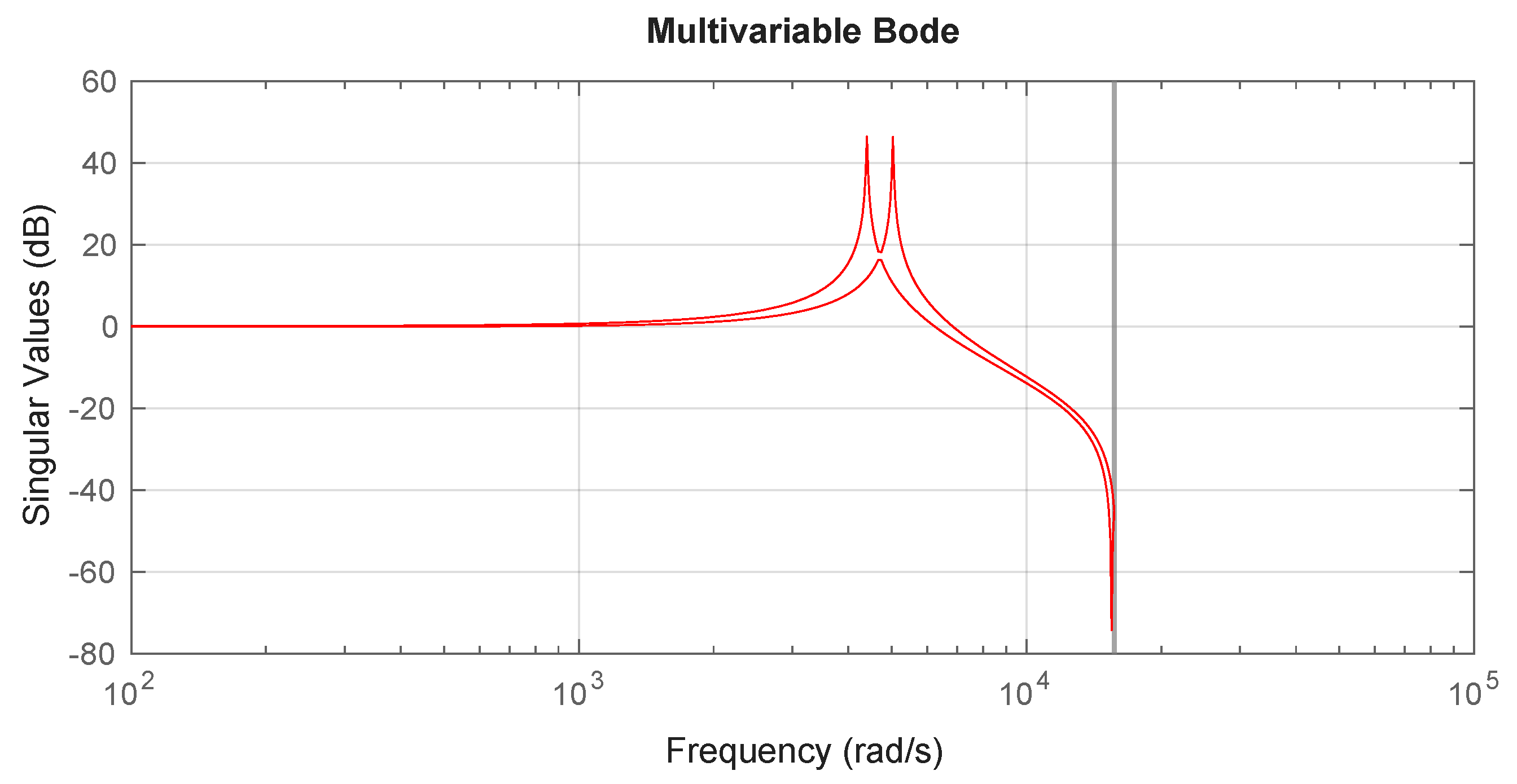
The discrete-time model in (6) serves as the foundation for constructing the prediction model required for MPC control. This work uses the multivariable frequency response of the model in (6) to establish design criteria for the closed-loop control. Figure 4 illustrates the eigenvalues that define the bandwidth of the open-loop system. Although the model is stable, it exhibits resonance points near 4500 rad/s and 5000 rad/s. Therefore, the control design must ensure robustness to effectively mitigate these oscillations at the resonant frequency. Moreover, it is essential to impose current constraints considering the nominal current of the VSI’s power semiconductors and ensure a feasible modulation voltage for safe operation. The voltage magnitude constraints at the converter output, which serves as the input to the LC filter, along with the system’s current constraints, are used to formulate the MPC optimization problem. The MPC formulation requires that the constraints be expressed as linear inequalities using the QP approach [15,21]. However, controlling the VSI in $dq$ coordinates introduces specific challenges. To overcome these issues, this work adopts the approximations proposed in [29], using polygonal restrictions to the modulated voltage and current restrictions. 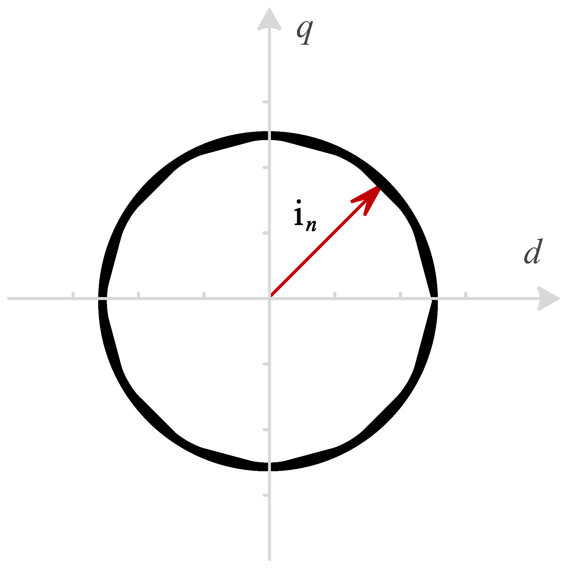To ensure the operation of the current within the nominal range, it is crucial to limit the output current of the converter (${\mathbf{i}}_{\mathrm{fdq}}$) within a circular boundary of radius $r=i_{\mathrm{n}}$, where $i_{\mathrm{n}}$ is the nominal current of the inverter. As discussed previously, these constraints must be reformulated as linear inequalities. In this study, this is achieved by approximating the circle with a regular dodecagon, as depicted in Figure 5. The current generation capacity accounts for 95.5% of the total circumference, with the remainder sacrificed due to the approximation. This strategy ensures rapid and robust control and maintains safe operation within the limits of the semiconductor. However, it involves a trade-off between the current restriction design’s precision and the optimization solver’s computational cost. The current constraints ${\mathbf{i}}_{\mathrm{fdq}}$ shown in Figure 5 can be expressed as inequality constraints by utilizing trigonometric identities, as follows:

$$\begin{array}{cc}\hfill {\mathbf{l}}_{\mathrm{x}}& \le \mathbf{J}{\mathbf{x}}_k\le {\mathbf{u}}_{\mathrm{x}},\hfill \end{array}$$

(8)

where the vectors and matrices are given by the following:

$$\begin{array}{cc}\hfill {\mathbf{l}}_{\mathrm{x}}& =i_{\mathrm{n}}\left[\begin{array}{c}3.73\\ 1.36\\ 1.00\\ 1.00\\ 1.36\\ 3.73\end{array}\right],\mathbf{J}=\left[\begin{array}{cccc}3.73& 1.00& 0.00& 0.00\\ 1.00& 1.00& 0.00& 0.00\\ 0.27& 1.00& 0.00& 0.00\\ -0.27& 1.00& 0.00& 0.00\\ -1.00& 1.00& 0.00& 0.00\\ -3.73& 1.00& 0.00& 0.00\end{array}\right]{\mathbf{u}}_{\mathrm{x}}=-{\mathbf{l}}_{\mathrm{x}}.\hfill \end{array}$$

(9)

In (8), the current constraints are represented using a constant matrix ($\mathbf{J}$) and a vector parameterized by $i_{\mathrm{n}}$, allowing generalization for various VSI generation capacities.

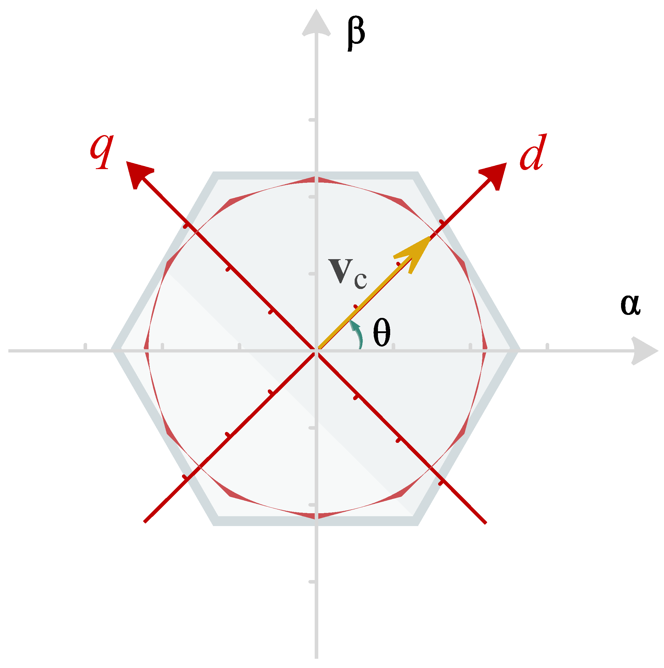
The voltage actuation, on the other hand, is achieved using space vector pulse width modulation (SV-PWM). This technique is widely employed in power electronics and is readily implemented in digital signal processors. The objective of the SV-PWM modulator is to generate a pulsed voltage with the desired average value, ensuring constant switching frequency and optimal utilization of the DC bus voltage. SV-PWM achieves approximately 15% greater utilization of the DC bus voltage compared to sinusoidal PWM techniques [30]. When the Clarke transformation is applied to all modulated inverter voltages, $v_{\mathrm{s}\alpha \beta ,t}=v_{\mathrm{s}\alpha ,t}+j{v}_{\mathrm{s}\beta ,t}$, these voltages are constrained within the hexagon defined by the six active vectors of the inverter, as illustrated in Figure 6. These constraints can be formulated as constant linear inequalities in the $\alpha \beta$ frame. However, the control of the inverter with an LC filter is performed in the $dq$ frame, requiring the rotation of these constraints. This results in $\theta$-dependent, time-varying constraints [29], which can be expressed in the $dq$ frame but involve a high computational cost. To avoid this cost, the voltage is limited to the circle inscribed within the hexagon, approximated using the same method applied to the filter current, i.e., with a dodecagon in $dq$ coordinates, as illustrated in Figure 6. These voltage constraints can be expressed as inequality constraints in $dq$ using (10).

$$\begin{array}{cc}\hfill {\mathbf{l}}_{\mathrm{u}}& \le \mathbf{E}{\mathbf{u}}_k\le {\mathbf{u}}_{\mathrm{u}},\hfill \end{array}$$

(10)

where the vectors and matrices are given by the following:

$$\begin{array}{cc}\hfill {\mathbf{l}}_{\mathrm{u}}& ={\displaystyle \frac{v_{\mathrm{dc}}}{\sqrt{3}}}\left[\begin{array}{c}3.73\\ 1.36\\ 1.00\\ 1.00\\ 1.36\\ 3.73\end{array}\right],\mathbf{E}=\left[\begin{array}{cc}3.73& 1.00\\ 1.00& 1.00\\ 0.27& 1.00\\ -0.27& 1.00\\ -1.00& 1.00\\ -3.73& 1.00\end{array}\right]{\mathbf{u}}_{\mathrm{u}}=-{\mathbf{l}}_{\mathrm{u}}.\hfill \end{array}$$

(11)

In (10), the modulated voltage constraints are represented using a constant matrix ($\mathbf{E}$) and a vector parameterized by $v_{\mathrm{dc}}$, allowing for generalization across VSIs with different DC-link voltages. The following sections detail the control design based on the model (6) and describe how the constraints in (8) and (10) are incorporated into the proposed MPC strategy.

4. Optimal Control Problem with Reference Tracking of the VSI Output Voltage

This section introduces reference tracking for the capacitor voltage magnitude using the linear quadratic regulator with integral action (LQI) method [31]. The integral action aims to reject the unmodeled errors and the disturbances in the system described in (6). To achieve this, newly expanded states are introduced to include the integral of the desired tracking error. The dynamic model of the augmented estates is given by the following:

$$\begin{array}{c}\hfill \left[\begin{array}{c}{s}_{1,t+1}\\ s_{2,t+1}\end{array}\right]=\left[\begin{array}{c}{s}_{1,t}\\ s_{2,t}\end{array}\right]+({\mathbf{y}}_t-\mathbf{r}).\end{array}$$

(12)

where ${\left[\begin{array}{cc}{s}_{1,t}& s_{2,t}\end{array}\right]}^{\top }$ are the expanded states and $\mathbf{r}$ is the voltage reference. Using (12) and treating the output current (${\mathbf{i}}_{\mathbf{o}}$) as an unmeasured disturbance, the model in (6) is expanded as follows:

$$\begin{array}{c}\hfill \begin{array}{cc}\hfill {\mathbf{x}}_{\mathrm{e},t+1}& ={\mathbf{A}}_e{\mathit{x}}_{\mathrm{e},t}+{\mathbf{B}}_{\mathrm{e}}{\mathbf{u}}_t+{\mathbf{B}}_{\mathrm{pe}}{\mathbf{i}}_{\mathrm{o},t},\hfill \\ \hfill {\mathbf{y}}_t& ={\mathbf{C}}_{\mathrm{e}}{\mathbf{x}}_{\mathrm{pe},t},\hfill \end{array}\end{array}$$

(13)

where the augmented state is ${\mathbf{x}}_{\mathrm{e},t}={[i_{\mathrm{fd},t},i_{\mathrm{fq},t},v_{\mathrm{cd},t},v_{\mathrm{cq},t},s_{1,t},s_{2,t}]}^{\top }$, and the matrices of the augmented system are as follows:

$$\begin{array}{c}\hfill {\mathbf{A}}_{\mathrm{e}}=\left[\begin{array}{cc}{\mathbf{A}}_{\mathrm{d}}& {\mathbf{0}}_{4\times 2}\\ \mathbf{C}& {\mathbb{I}}_{2\times 2}\end{array}\right],{\mathbf{B}}_{\mathrm{e}}=\left[\begin{array}{c}{\mathbf{B}}_{\mathrm{d}}\\ {\mathbf{0}}_{2\times 2}\end{array}\right],{\mathbf{B}}_{\mathrm{pe}}=\left[\begin{array}{c}{\mathbf{B}}_{\mathrm{dp}}\\ {\mathbf{0}}_{2\times 2}\end{array}\right],{\mathbf{C}}_{\mathrm{e}}=\left[\begin{array}{cc}\mathbf{C}& {\mathbf{0}}_{2\times 2}.\end{array}\right]\end{array}$$

(14)

The control feedback matrix is obtained by solving the following optimization problem:

$$\begin{array}{cc}\hfill min& \sum _{k=0}^{\infty }\left({\mathbf{x}}_{\mathrm{e},k}^{\top }\mathbf{Q}{\mathbf{x}}_{\mathrm{e},k}+{\mathbf{u}}_{\mathrm{e},k}^{\top }\mathbf{R}{\mathbf{u}}_{\mathrm{e},k}\right),\hfill \end{array}$$

(15)

$$\begin{array}{cc}\hfill \mathrm{s}.\mathrm{t}.& {\mathbf{x}}_{\mathrm{e},k+1}={\mathbf{A}}_{\mathrm{e}}{\mathbf{x}}_{\mathrm{e},k}+{\mathbf{B}}_{\mathrm{e}}{\mathbf{u}}_k,\hfill \end{array}$$

(16)

where $\{\mathbf{Q},\mathbf{R}\}>0$ are weighting matrices that define the desired closed-loop performance of the system. Limiting the closed-loop system’s bandwidth is crucial to achieving a robust design and mitigating system resonances. Conversely, ensuring a sufficiently high bandwidth is essential for enhancing the dynamic performance of the control loop. This trade-off is addressed by adjusting the values of $\mathbf{Q}$ and $\mathbf{R}$. Following the methodology proposed in [32], the matrices are adjusted as $\mathbf{Q}=\mathrm{diag}({\mathbb{I}}_{4\times 4},{\rho }_1{\mathbb{I}}_{2\times 2})$ and $\mathbf{R}={\mathbb{I}}_{2\times 2}$. Consequently, the control design is simplified to tuning the parameter ${\rho }_1$ to achieve the desired closed-loop bandwidth. The LQI control law is given by the following:

$$\begin{array}{c}\hfill {\mathbf{u}}_t=-{\mathbf{K}}_{\infty }{\mathbf{x}}_{\mathrm{e},t},\end{array}$$

(17)

with ${\mathbf{K}}_{\infty }=({\mathbf{B}}_{\mathrm{e}}^{\mathrm{T}}\mathbf{S}{\mathbf{B}}_{\mathrm{e}}+{\mathbf{R}}^{-1}\left({\mathbf{B}}_{\mathrm{e}}^{\mathrm{T}}\mathbf{S}{\mathbf{A}}_{\mathrm{e}}^{\mathrm{T}}\right)$ the optimal gain matrix, and $\mathbf{S}$ the solution to the Riccati, and the closed-loop system transition matrix is given by the following:

$${\mathbf{A}}_{\mathrm{closed}}={\mathbf{A}}_{\mathrm{e}}-{\mathbf{B}}_{\mathrm{e}}·{\mathbf{K}}_{\infty }.$$

(18)

Figure 7 illustrates the multivariable frequency response of the closed-loop system with the parameter ${\rho }_1=1e-2$. This design criterion ensures the damping of critical frequencies near 4500 rad/s and 5000 rad/s, and cero db gain at dc, i.e., achieving reference tracking at steady state. However, it is essential to reformulate this problem as a constrained QP optimization problem to incorporate the system constraints described in (8) and (10). The next section introduces the MPC framework to address this requirement. This leads to a constrained MPC formulation with explicit integration [33].

5. Model-Based Predictive Control of the VSI

The model in (6) and the inequality constraints in (8) and (10) are used to formulate the control algorithm as a quadratic programming (QP) problem, based on the following quadratic cost function [33]:

$$\begin{array}{c}\hfill V(\tilde{\mathbf{x}},\tilde{\mathbf{u}})={\tilde{\mathbf{x}}}_{\mathrm{e},N}^{\top }{\mathbf{Q}}_N{\tilde{\mathbf{x}}}_{\mathrm{e},N}+\sum _{k=0}^{N-1}{\tilde{\mathbf{x}}}_{\mathrm{e},k}^{\top }\mathbf{Q}{\tilde{\mathbf{x}}}_{\mathrm{e},k}+{\tilde{\mathbf{u}}}_k^{\top }\mathbf{R}{\tilde{\mathbf{u}}}_k,\end{array}$$

(19)

where $\mathbf{Q}$ and $\mathbf{R}$ are the same weighting matrices for the state and input defined of (15), and ${\mathbf{Q}}_N$ is the solution of the discrete-time Riccati equation associated with the optimal control problem. This criterion ensures system stability while maintaining the same dynamic response as the LQI when the constraints are not active. The prediction horizon is N, and $\{{\tilde{\mathbf{x}}}_{\mathrm{e},k},{\tilde{\mathbf{u}}}_k\}$ represent deviation variables around de desired steady-state operating point,

$$\begin{array}{cc}\hfill {\tilde{\mathbf{x}}}_{\mathrm{e},k}& ={\mathbf{x}}_{\mathrm{e},t}-\left[\begin{array}{c}{\overline{\mathbf{x}}}_{\mathrm{s}}\\ {\mathbf{0}}_{2\times 1}\end{array}\right],\hfill \end{array}$$

(20)

$$\begin{array}{cc}\hfill {\tilde{\mathbf{u}}}_k& ={\mathbf{u}}_t-{\overline{\mathbf{u}}}_{\mathrm{s}}.\hfill \end{array}$$

(21)

The steady-state operating point $\{{\overline{\mathbf{x}}}_{\mathrm{s}},{\overline{\mathbf{u}}}_{\mathrm{s}}\}$ is computed as follows:

$$\begin{array}{c}\hfill \left[\begin{array}{c}{\overline{\mathbf{x}}}_{\mathrm{s}}\\ {\overline{\mathbf{u}}}_{\mathrm{s}}\end{array}\right]={\left[\begin{array}{cc}{\mathbb{I}}_{4\times 4}-{\mathbf{A}}_{\mathrm{d}}& -{\mathbf{B}}_{\mathrm{d}}\\ \mathbf{C}& {\mathbf{0}}_{2\times 2}\end{array}\right]}^{-1}\left[\begin{array}{c}{\mathbf{B}}_{\mathrm{pd}}{\mathbf{i}}_{\mathrm{o},t}\\ \mathbf{r}\end{array}\right].\end{array}$$

(22)

The state and input constraints are given by the following:

$$\begin{array}{cc}\hfill {\tilde{\mathbf{x}}}_{e,k+1}& ={\mathbf{A}}_{\mathrm{e}}{\tilde{\mathbf{x}}}_{e,k}+{\mathbf{B}}_{\mathrm{e}}{\tilde{\mathbf{u}}}_k,\hfill \end{array}$$

(23)

$$\begin{array}{cc}\hfill {\tilde{\mathbf{x}}}_{\min }& \le {\mathbf{J}}_{\mathbf{e}}{\tilde{\mathbf{x}}}_k\le {\tilde{\mathbf{x}}}_{\max },\hfill \end{array}$$

(24)

$$\begin{array}{cc}\hfill {\tilde{\mathbf{u}}}_{\min }& \le \mathbf{E}{\tilde{\mathbf{u}}}_k\le {\tilde{\mathbf{u}}}_{\max },\hfill \end{array}$$

(25)

$$\begin{array}{cc}\hfill {\mathbf{x}}_0& ={\mathbf{x}}_t,\hfill \end{array}$$

(26)

where ${\mathbf{J}}_{\mathbf{e}}=\left[\begin{array}{cc}\mathbf{J}& {\mathbf{0}}_{6\times 2}\end{array}\right]$, and (24) and (25) represent the states and inputs constraints using the transformations (20) and (21). The control action is computed by solving the optimization problem and using a receding horizon scheme (RHC) at time t. This approach accelerates the steady state convergence of the system by forwarding the steady state operating point, using the references and known disturbances, improving the system’s time response. However, when current constraints are active, the integral of the error between the voltage and its references becomes an open integrator, leading to numerical problems in the MPC control. To address this challenge, this work adopts the incremental formulation proposed in [34].

Incremental Formulation

Following the MPC formulation presented in [34], the quadratic cost function can be rewritten as follows:

$$\begin{array}{c}\hfill V_2(\tilde{\mathbf{x}},\tilde{\mathbf{u}})=\Delta {\tilde{\mathbf{x}}}_{\mathrm{e},N}^{\top }{\mathbf{Q}}_N\Delta {\tilde{\mathbf{x}}}_{\mathrm{e},N}+\sum _{k=0}^{N-1}\Delta {\tilde{\mathbf{x}}}_{\mathrm{e},k}^{\top }\mathbf{Q}\Delta {\tilde{\mathbf{x}}}_{\mathrm{e},k}+\Delta {\tilde{\mathbf{u}}}_k^{\top }\mathbf{R}\Delta {\tilde{\mathbf{u}}}_k,\end{array}$$

(27)

where,

$$\begin{array}{cc}\hfill \Delta {\tilde{\mathbf{x}}}_{\mathrm{e},k}& =\left[\begin{array}{c}{\tilde{\mathbf{x}}}_t\\ {\mathbf{y}}_{t-1}\end{array}\right]-\left[\begin{array}{c}{\tilde{\mathbf{x}}}_{\mathbf{t}-\mathbf{1}}\\ \mathbf{r}\end{array}\right],\hfill \end{array}$$

(28)

$$\begin{array}{cc}\hfill \Delta {\tilde{\mathbf{u}}}_k& ={\tilde{\mathbf{u}}}_t-{\tilde{\mathbf{u}}}_{t-1},\hfill \end{array}$$

(29)

represent the incremental variables. Given these transformations, the state and input constraints are given by the following:

$$\begin{array}{c}\hfill \begin{array}{cc}\hfill \Delta {\tilde{\mathbf{x}}}_{e,k+1}& ={\mathbf{A}}_{\mathrm{e}}\Delta {\tilde{\mathbf{x}}}_{e,k}+{\mathbf{B}}_{\mathrm{e}}\Delta {\tilde{\mathbf{u}}}_k,\hfill \\ \hfill \Delta {\tilde{\mathbf{x}}}_{\min }& \le \mathbf{J}\Delta {\tilde{\mathbf{x}}}_k\le \Delta {\tilde{\mathbf{x}}}_{\max },\hfill \\ \hfill \Delta {\tilde{\mathbf{u}}}_{\min }& \le \mathbf{E}\Delta {\tilde{\mathbf{u}}}_k\le \Delta {\tilde{\mathbf{u}}}_{\max },\hfill \\ \hfill {\mathbf{x}}_0& ={\mathbf{x}}_t,\hfill \end{array}\end{array}$$

(30)

where

$$\begin{array}{cc}\hfill \Delta {\tilde{\mathbf{x}}}_{\min }& ={\mathbf{l}}_{\mathrm{x}}-\mathbf{J}({\mathbf{x}}_{k-1}+\Delta {\overline{\mathbf{x}}}_{\mathrm{s},t}),\hfill \end{array}$$

(31)

$$\begin{array}{cc}\hfill \Delta {\tilde{\mathbf{x}}}_{\max }& ={\mathbf{u}}_{\mathrm{x}}-\mathbf{J}({\mathbf{x}}_{k-1}+\Delta {\overline{\mathbf{x}}}_{\mathrm{s},t}),\hfill \end{array}$$

(32)

$$\begin{array}{cc}\hfill \Delta {\tilde{\mathbf{u}}}_{\min }& ={\mathbf{l}}_{\mathrm{u}}-\mathbf{E}({\mathbf{u}}_{k-1}+\Delta {\overline{\mathbf{u}}}_{\mathrm{s},t}),\hfill \end{array}$$

(33)

$$\begin{array}{cc}\hfill \Delta {\tilde{\mathbf{u}}}_{\max }& ={\mathbf{u}}_{\mathrm{u}}-\mathbf{E}({\mathbf{u}}_{k-1}+\Delta {\overline{\mathbf{u}}}_{\mathrm{s},t}).\hfill \end{array}$$

(34)

The optimization problem must be reformulated to a standard form to be compatible with the OSQP solver [25], as follows:

$$\begin{array}{cc} min\hfill & {\displaystyle \frac{1}{2}}{\mathit{\psi }}^{\top }\mathbf{H}\mathit{\psi }+{\mathbf{h}}^{\top }\mathit{\psi },\hfill \end{array}$$

(35)

$$\begin{array}{cc}\mathrm{s}.\mathrm{t}.\hfill & \mathbf{F}\mathit{\psi }=\mathbf{f},\hfill \end{array}$$

(36)

$$\begin{array}{cc}\hfill & \mathbf{a}\le \mathbf{P}\mathit{\psi }\le \mathbf{b}.\hfill \end{array}$$

(37)

There are two mathematically equivalent alternatives to express the problem (27)–(34): the condensed and non-condensed approaches [35]. However, each approach offers different numerical properties [35]. Following the more intuitive non-condensed approach, the problem of interest is described as follows:

$$\begin{array}{cc}\hfill \mathit{\psi }& =\left[\begin{array}{c}\Delta {\tilde{\mathbf{x}}}_o\\ ⋮\\ \Delta {\tilde{\mathbf{x}}}_N\\ \Delta {\tilde{\mathbf{u}}}_o\\ ⋮\\ ⋮\\ {\tilde{\mathbf{u}}}_{N-1}\end{array}\right],\mathbf{H}=\left[\begin{array}{ccccccc}\mathbf{Q}& \mathbf{0}& \mathbf{0}& \mathbf{0}& \cdots & \mathbf{0}& \mathbf{0}\\ \mathbf{0}& \ddots & \mathbf{0}& \mathbf{0}& \mathbf{0}& \cdots & ⋮\\ \mathbf{0}& \mathbf{0}& \mathbf{Q}& \mathbf{0}& \mathbf{0}& \cdots & ⋮\\ \mathbf{0}& \mathbf{0}& \mathbf{0}& {\mathbf{Q}}_N\mathbf{0}& \cdots & ⋮\\ ⋮& ⋮& ⋮& \mathbf{0}& \mathbf{R}& ⋮& ⋮\\ \mathbf{0}& \cdots & \cdots & \cdots & \cdots & \ddots & ⋮\\ \mathbf{0}& \cdots & \cdots & \cdots & \cdots & \cdots & \mathbf{R}\end{array}\right],\hfill \end{array}$$

(38)

$\mathit{\psi }$ is the decision vector, $\mathbf{H}$ is the Hessian matrix, and $\mathbf{h}\in$ is a zero column vector. The initial condition of the QP problem and the predictive model (16) are formulated as the equality constraints in (36) with the following:

$$\begin{array}{c}\hfill \mathbf{F}=\left[\begin{array}{ccccc}-{\mathbb{I}}_{6\times 6}& \mathbf{0}& \mathbf{0}& \cdots & \mathbf{0}\\ {\mathbf{A}}_{\mathrm{e}}& -{\mathbb{I}}_{6\times 6}& \mathbf{0}& {\mathbf{B}}_{\mathrm{e}}& \mathbf{0}\\ \mathbf{0}& {\mathbf{A}}_{\mathrm{e}}& -{\mathbb{I}}_{6\times 6}& \ddots & {\mathbf{B}}_{\mathrm{e}}\\ ⋮& \ddots & \ddots & \ddots & \ddots \\ \mathbf{0}& \cdots & \cdots & \cdots & \cdots \end{array}\right],\mathbf{f}=\left[\begin{array}{c}-\Delta {\tilde{\mathbf{x}}}_0\\ \mathbf{0}\\ \mathbf{0}\\ ⋮\\ \mathbf{0}\end{array}\right].\end{array}$$

(39)

The constraint in (39) represents the current behavior of the system while forecasting its future dynamics over N steps to ensure optimal performance. The constraints on the LC filter current and the modulated voltage are formulated as the inequality constraints in (37), where

$$\begin{array}{c}\hfill \mathbf{P}=\left[\begin{array}{cccccc}{\mathbf{J}}_{\mathbf{e}}& \mathbf{0}& \mathbf{0}& \mathbf{0}& \cdots & \mathbf{0}\\ \mathbf{0}& \ddots & \mathbf{0}& \mathbf{0}& \cdots & \mathbf{0}\\ \mathbf{0}& \mathbf{0}& {\mathbf{J}}_{\mathbf{e}}& \mathbf{0}& \cdots & \mathbf{0}\\ \mathbf{0}& \mathbf{0}& \mathbf{0}& \mathbf{E}& \cdots & \mathbf{0}\\ ⋮& ⋮& ⋮& ⋮& \ddots & \mathbf{0}\\ \mathbf{0}& \mathbf{0}& \mathbf{0}& \mathbf{0}& \mathbf{0}& \mathbf{E}\end{array}\right],\mathbf{a}=\left[\begin{array}{c}\Delta {\tilde{\mathbf{x}}}_{\min }\\ ⋮\\ \Delta {\tilde{\mathbf{x}}}_{\min }\\ \Delta {\tilde{\mathbf{u}}}_{\min }\\ ⋮\\ \Delta {\tilde{\mathbf{u}}}_{\min }\end{array}\right],\mathbf{b}=\left[\begin{array}{c}\Delta {\tilde{\mathbf{x}}}_{\max }\\ ⋮\\ \Delta {\tilde{\mathbf{x}}}_{\max }\\ \Delta {\tilde{\mathbf{u}}}_{\max }\\ ⋮\\ \Delta {\tilde{\mathbf{u}}}_{\max }\end{array}\right].\end{array}$$

(40)

Solving the optimization problem (35), subject to the constraints (36) and (37), the algorithm computes the MPC output thought the OSQP solver using the RHC approach:

$$\begin{array}{c}\hfill \Delta {\tilde{\mathbf{u}}}_0=\mathrm{OSQP}(\mathbf{H},\mathbf{h},\mathbf{F},\mathbf{f},\mathbf{P},\mathbf{a},\mathbf{b}),\end{array}$$

(41)

where the control of the system is given by the following:

$$\begin{array}{c}\hfill {\mathbf{u}}_t=\Delta {\tilde{\mathbf{u}}}_0+{\mathbf{u}}_{t-1}+\Delta {\overline{\mathbf{u}}}_{\mathrm{s},t}.\end{array}$$

(42)

Interested readers are encouraged to consult [25] for more information on the OSQP solver. The proposed control strategy in (42) achieves reference tracking of the capacitor voltage in the VSI. Additionally, it accounts for operational constraints on the modulated voltage and physical limitations of the filter current through a QP approach. Including deviation variables in the MPC accelerates the system’s steady-state convergence by feed-forwarding the steady-state operating point, thereby feeding forward the reference and the known disturbances and improving the system’s time response. For embedded implementation, this work reformulates the equivalent optimization problem using the condensed approach for a more efficient implementation [35], achieving reduced computational costs and enabling average solution times of 70 μs. Details of the condensed implementation are provided in Appendix A.

6. Results

This section presents the results of controlling a VSI using the proposed strategy detailed in Section 5. Specifically, the tests assess the performance of the MPC controller, designed with a prediction horizon $N=2$, derived from the system’s dynamic model and extended with integral action [34], in achieving offset-free voltage reference tracking. Additionally, the analysis evaluates the system’s compliance with operational and physical limitations, which are incorporated into the MPC formulation as linear constraints. The proposed approach is first tested through MATLAB simulations to evaluate its functionality. Finally, experimental results are presented to validate the proposed method.

To evaluate its performance, a simulation comparison is conducted with a conventional cascaded PI control strategy presented in [36]. The system parameters used in this work are summarized in Table 1, and correspond to the experimental setup in the electronic power laboratory discussed in Section 2.

6.1. Simulation Results

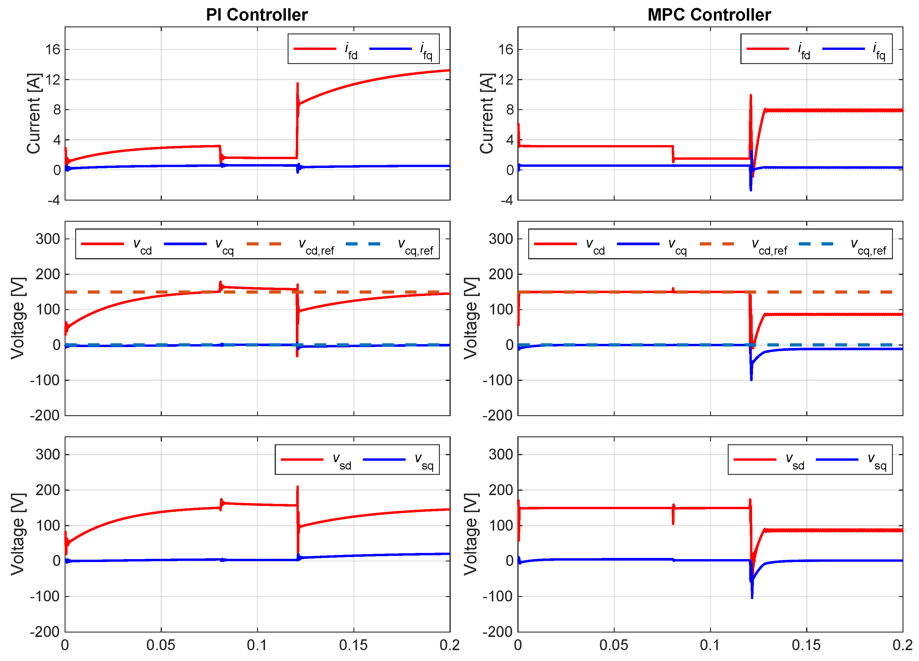
The time-response simulations are performed in MATLAB. Figure 8 presents the simulation results in the $dq$ reference frame, with the hierarchical control response based on PIs shown on the left and the response of the proposed MPC strategy displayed on the right. Initially, the VSI supplies a resistive load of $47\mathsf{\Omega }$ with a reference voltage of $150\mathrm{V}$. Both control strategies achieve offset-free behavior due to the integral action. However, the MPC approach achieves steady-state operation faster than the PI-based approach, demonstrating improved settling time. At $t=0.07\mathrm{s}$, the resistive load is increased to $100\mathsf{\Omega }$ to evaluate the system’s response to load changes when no constraints are active. The MPC response is almost instantaneous, attributed to the feed-forward compensation of the measured disturbance, ${\mathbf{i}}_{\mathbf{o}}$.

At $t=0.12\mathrm{s}$, the load resistance is changed to $11\mathsf{\Omega }$ to evaluate compliance with the current limitation depicted in Figure 5. The MPC controller effectively enforces the steady-state current limit of $8\mathrm{A}$ by reducing the modulated voltage (${\mathbf{v}}_{\mathrm{sdq}}$). Additionally, the MPC demonstrates improved settling time compared to the PI controllers. While transient responses briefly exceed the limits, the PI controllers exhibit significantly higher overshoot and are unable to restrict the load current effectively.

6.2. Experimental Results

This section presents the VSI control of the experimental setup illustrated in Figure 3. The MPC is formulated as a QP problem, as described in Section 5, and implemented in C code using the OSQP solver [25,37]. The RHC computes the MPC control input, which is transformed back to $abc$ coordinates (${\mathbf{v}}_{\mathrm{abc}}$). The inverter pulses are generated using the space vector pulse-width modulator (SVPWM) in the dSPACE system. The human–machine interface (HMI) displays the voltage magnitude, filter current, output current, and execution time of the MPC algorithm in the ControlDesk software, enabling the evaluation of the VSI’s dynamic performance and computational cost.

This work evaluates the performance of the OSQP solver under various important operating conditions. Specifically, it focuses on voltage reference tracking and the activation of constraints for modulated voltage and filter current. In all cases, the iterative computation of voltage actuation is performed with 10 iterations, allowing the OSQP solver to achieve the solution in an average time of $70\mathsf{\mu }$s, demonstrating its suitability for MPC implementation in VSI control with the target sampling time of $200\mathsf{\mu }$s. For simplicity in the experimental tests, the steady-state values in the MPC algorithm design are set to zero, i.e., ${\overline{\mathbf{x}}}_{\mathrm{s}}=\mathbf{0}$ and ${\overline{\mathbf{u}}}_{\mathrm{s}}=\mathbf{0}$. Although this decision slows the system’s convergence to a steady state, offset-free performance is ensured by the integral action included in the control design.

6.3. Voltage Magnitude Reference Tracking

Figure 9 illustrates the filter current, output current, and capacitor voltage in $abc$ coordinates, highlighting the VSI’s voltage tracking response to the capacitor voltage reference. The modulated voltage and current constraints are represented by dashed lines. At $t=2.60$ s, a step voltage reference is applied, resulting in an output voltage of $120\mathrm{V}$. The MPC controller successfully tracks the desired reference voltage, demonstrating the fast response of the proposed control strategy.

6.4. Modulated Voltage Constraints

Figure 10 illustrates the VSI transient response under active modulated voltage constraints. The voltage amplitude constraint is fixed to $138\mathrm{V}$ and originally the system operates in the unconstrained region with a reference of $120\mathrm{V}$. At $t=2.75$ s; the voltage reference is changed to $150\mathrm{V}$ exceeding the specified restriction. In this case, the filter current and modulated voltage are constrained to ensure compliance with the imposed limits, even when the reference signal exceeds the defined limit. The experimental results show that the modulated voltage remains within the specified limits enforced by the MPC control strategy.

6.5. Filter Current Restriction

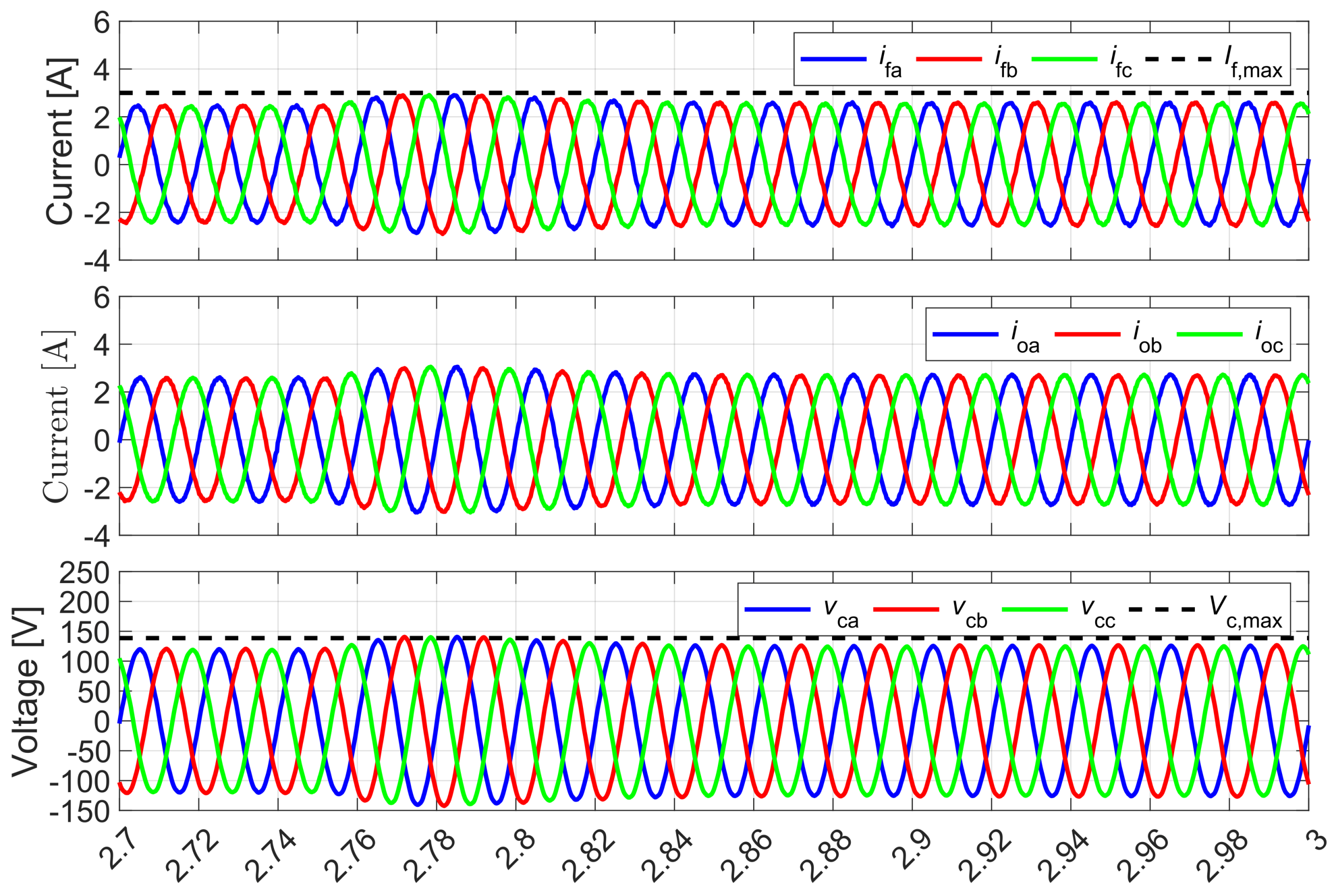
Figure 11 illustrates the VSI response when current limit constraints are activated. Initially, the VSI operates with an output voltage of $100\mathrm{V}$, supplying a load resistance of $47\mathsf{\Omega }$ and a current limit of $3\mathrm{A}$, i.e., in unconstrained operation mode. At $t=2.66\mathrm{s}$, a load breaker is closed, connecting an additional bank of $23\mathsf{\Omega }$ load resistances in parallel, activating the current limit. During the transient response, the current constraint is briefly exceeded due to large output current disturbances. The algorithm responds by reducing the output voltage, albeit at a limited rate, resulting in a transient overcurrent. However, the MPC controller quickly adjusts the modulated voltage to ensure that the output current remains within the predefined limit of $3\mathrm{A}$ in steady state, as set by the current constraints.

7. Discussion

Advancements in computational resources have enabled the application of MPC in systems requiring high dynamic performance, such as VSI control. Unlike conventional control strategies, MPC can predict system behavior and incorporate operational constraints directly into control design. In this context, the proposed MPC computes the optimal control action to achieve the voltage magnitude reference while considering filter current and voltage modulation constraints. Additionally, the method leverages an augmented system to incorporate integral action, improving steady-state accuracy, and utilizes the system’s steady-state behavior to enhance the transient response, ensuring faster convergence.

This article presents an offset-free MPC for the VSI using the OSQP solver, which efficiently solves the resulting QP problem. The computational cost is evaluated on the dSPACE MicroLabBox platform, demonstrating the feasibility of this approach via the condensed problem formulation. The proposed methodology is applicable to voltage control in DERs within microgrids, meeting the growing demand for advanced control strategies in modern decentralized power systems. This control approach could be extended to higher-level control loops in microgrids [38], such as secondary control, to achieve reference tracking of voltage and operating frequency while also incorporating operational constraints.

8. Conclusions

This work proposed an MPC technique with integral action for the control of voltage source inverters with LC filters in grid-connected applications and validated it in an experimental VSI setup. The control design enabled accurate reference tracking of the output voltage within the model predictive control framework while achieving a suitable transient response to load current disturbances. Furthermore, the method integrates operational constraints on the filter current and modulated voltage, providing effective protection for the power converter during grid faults or significant network transients. Simulation results conducted in MATLAB demonstrate the dynamic performance of the proposed MPC algorithm and its capability to protect critical power electronics assets in the grid, making it a superior alternative to traditional hierarchical PI controllers. Furthermore, the experimental implementation achieved resolution times for the resulting QP problem of less than 70 μs using the readily available OSQP solver, appropriately configured and tuned. This validates the feasibility of the proposed method for practical implementation in VSIs with LC filters for grid-connected applications. Finally, the experimental offset-free MPC could be explored for extension to higher closed-loop levels in the microgrid hierarchy that require integration, such as secondary control, to enhance stability, incorporate operational constraints, and ensure accurate voltage and frequency tracking.