SCS-JPGD: Single-Channel-Signal Joint Projected Gradient Descent

Abstract

The fault diagnosis of industrial equipment is crucial for ensuring production safety and improving the efficiency of equipment operation. With the advancement of sensor technologies, the number of data generated in industrial environments has increased dramatically. Deep learning techniques, with their powerful feature extraction and classification capabilities, have become a research hotspot in the field of fault diagnosis. However, deep learning models are vulnerable to adversarial attacks, which can lead to a decrease in diagnostic accuracy and compromise system safety. This paper proposes a Joint Projection Gradient Descent (SCS-JPGD) method based on single-channel signal features. The proposed method first introduces a gradient-based attack approach for signal samples, which can add tiny perturbations to the input samples, causing misclassification in black-box models. Secondly, a joint training strategy is proposed for gradient attacks on signal samples, aiming to enhance the model’s adaptability to small perturbations in a limited range. Experiments were conducted on the CWRU dataset under four different operating conditions. The results show that, under a deep learning model with diagnostic accuracy exceeding 90%, the joint training method allows the model to maintain an average accuracy of 84.6% even after the addition of adversarial samples, which are barely distinguishable by the human eye. The proposed SCS-JPGD method provides a safer and more accurate approach for fault diagnosis in deep learning research.

1. Introduction

The reliable operation of industrial equipment is crucial for ensuring production efficiency and safety, particularly in the fault diagnosis of critical components such as rotating bodies. Bearing faults are often detected through vibration signals, which typically account for a significant portion of the fault diagnosis in industrial equipment. Bearing vibration signals can reflect their operational status, but in the complex and dynamic industrial environment, traditional fault diagnosis methods that rely on expert knowledge and manual feature extraction struggle to effectively address the noise and nonlinear characteristics inherent in vibration signals. In recent years, deep learning techniques, with their ability to automatically extract features and perform efficient classification, have been widely applied in fault diagnosis, especially in the analysis of bearing vibration signals [1,2,3,4].

However, the security issues of deep learning models have increasingly attracted widespread attention. Specifically, deep learning models are vulnerable to adversarial attacks, leading to two main problems: on the one hand, malicious attacks may interfere with the model’s judgment through carefully designed adversarial samples, misguiding the fault diagnosis system and potentially creating safety hazards [5,6]; on the other hand, the model’s inability to accurately recognize even slight perturbations can also impact the reliability of diagnostic results [7,8]. Therefore, improving the robustness and generalization capability of deep learning models in fault diagnosis has become an urgent research topic.

In recent years, deep learning-based fault diagnosis methods have gradually become an important tool for industrial equipment monitoring. These methods, through automatic feature extraction and efficient classification capabilities, have significantly improved the accuracy and efficiency of fault detection. Common deep learning models include Convolutional Neural Networks (CNNs) [1,2,3,4], Long Short-Term Memory networks (LSTM) [3,9,10], and Recurrent Neural Networks (RNN) [11,12], which can effectively learn key features from raw data and, in turn, enhance the accuracy of fault diagnosis. However, the robustness of deep learning models has gradually become a concern when facing the complex and dynamic industrial environment. In practical applications, factors such as noise, sensor faults, data loss, and temperature changes often exist in industrial settings, which can affect the quality and stability of data, making it difficult for traditional deep learning models to guarantee stability and accuracy under these conditions.

To address these issues, researchers have proposed several methods to enhance robustness. Data augmentation techniques, by rotating, scaling, and adding noise to the training data, simulate the variable conditions in actual industrial environments, thereby improving the model’s adaptability to uncertainty [13,14]; adversarial training methods, by introducing adversarial samples with intentionally crafted perturbations during the training process, enable the model to learn more robust features and improve its resistance to disturbances [15,16]; simultaneously, regularization techniques are widely applied in deep learning models to reduce overfitting and improve the generalization ability of the model across different environments [17,18]. Additionally, techniques combining self-supervised learning and transfer learning have also been increasingly applied to fault diagnosis tasks, further enhancing the model’s robustness in small-sample data scenarios and dynamically changing environments.

Despite the improvements these methods have made in model robustness, the sensitivity of deep learning models to input data remains a critical issue. Especially when facing extreme disturbances or adversarial attacks, traditional methods still struggle to ensure model stability, potentially leading to severe deviations in fault diagnosis results and even posing safety risks. In the defense against adversarial attacks, traditional methods such as the Fast Gradient Sign Method (FGSM) [5,7] and Projected Gradient Descent (PGD) have been widely applied. Compared to FGSM, PGD can perform multiple iterations during the optimization process, generating stronger adversarial samples. However, although PGD has achieved certain results in defense, and it may introduce excessive interference during the training process, leading to decreased training efficiency. Therefore, this paper proposes a method based on vibration signal Convolutional Neural Networks (CNNs) and adversarial training. By introducing PGD-based adversarial attacks to generate adversarial samples and incorporating these samples into the training process, the model’s resistance to disturbances is enhanced. The main contributions of this paper are as follows.

1.

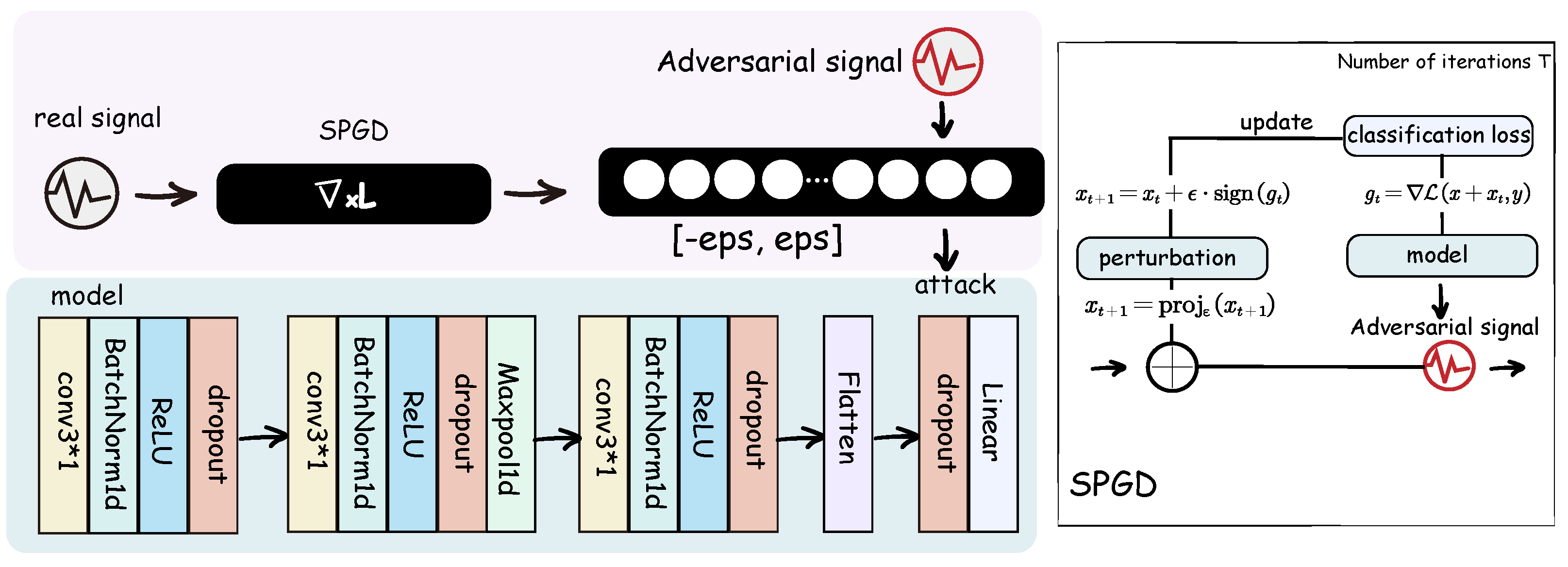
A novel and effective adversarial sample generation method based on the Projected Gradient Descent attack is proposed, which can introduce sufficient interference to the model.

2.

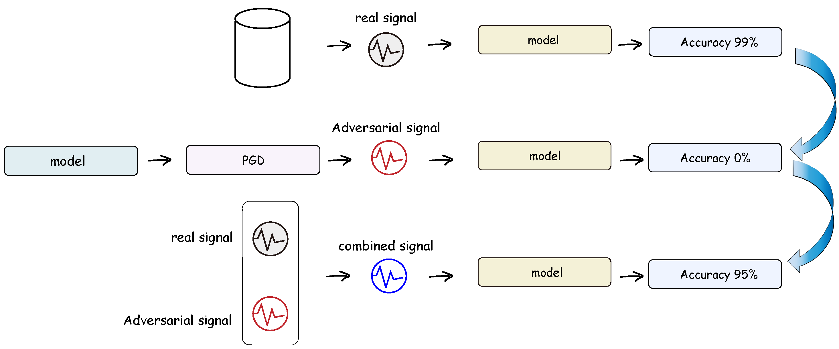
A joint training approach under gradient-based adversarial attacks is introduced, which allows the model to undergo adversarial training and regain high diagnostic accuracy under minor perturbations.

3.

Comprehensive experiments were conducted on the CWRU dataset under four different operating conditions, achieving a classification accuracy of 90% and improving the model’s robustness.

2. Related Works

2.1. Application of Deep Learning in Fault Diagnosis

Deep learning techniques, particularly Convolutional Neural Networks (CNNs) and Recurrent Neural Networks (RNNs), have achieved remarkable success in the field of fault diagnosis. By automating feature extraction, deep learning models can effectively identify potential fault patterns from complex signals, significantly improving the accuracy and efficiency of fault detection. For instance, CNN-based models have demonstrated excellent performance in vibration signal analysis, capturing temporal features in the signals and accurately identifying fault types under different operating conditions, yielding outstanding results in fault diagnosis. For example, Ruan et al. [1] leveraged the physical characteristics of bearing acceleration signals to guide CNN design for model optimization. Liang et al. [2] proposed a 2-D hierarchical CNN (HCNN) hardware accelerator, implemented with 40 nm CMOS technology, for bearing fault diagnosis on the CWRU dataset. Fang et al. [3] introduced a fault diagnosis model based on Bayesian optimization (BO-CNN-LSTM). Anurag et al. [4] acquired raw vibration and acoustic signals at different speeds and used Constant-Q Nonstationary Gabor Transform (CQ-NSGT) to convert them into time-frequency spectra for fault diagnosis. Simultaneously, RNNs, particularly Long Short-Term Memory (LSTM) networks, have been widely applied in dynamic system fault diagnosis due to their ability to model long-term and short-term dependencies in sequential data. They can accurately capture dynamic changes in equipment and perform anomaly detection, providing reliable support for early warning. For example, An et al. [12] proposed an RNN-based model for time-varying operating condition fault diagnosis, while Gao et al. [9] considered a quasi-periodic, LSTM-based method for the weak fault diagnosis of rolling bearings. Chen et al. [10] proposed an automatic feature learning neural network that uses two Convolutional Neural Networks with different kernel sizes to automatically extract signal features from raw data at different frequencies. Through these technologies, deep learning models can effectively handle large-scale data processing needs and demonstrate strong generalization capabilities, adapting to various operating conditions and complex noise environments.

However, the application of deep learning models in fault diagnosis also faces certain challenges. The “black-box” nature of these models makes their decision-making process difficult to interpret [19,20], lacking transparency. Particularly when faced with noise, disturbances, and data missing issues, the models may lead to unstable diagnostic results, impacting the reliability and safety of the system. For instance, when equipment experiences atypical faults or significant changes in operating conditions, deep learning models may struggle to accurately identify these new types of faults, leading to misdiagnosis or missed diagnosis.

2.2. Adversarial Samples and Adversarial Training

In recent years, significant progress has been made in improving model reliability and robustness. For instance, SC Kuok et al. [21] explored how to optimize the architecture of non-parametric probabilistic modeling through extensive Bayesian learning (BBL) to enhance model robustness. This method provides stronger defenses by incorporating probabilistic modeling and Bayesian inference, particularly in situations where data are uncertain or incomplete. Cao et al. [22] analyzed the robustness of deep neural networks under noise disturbances, proposing a framework to evaluate the impact of different types of noise on the model, and improving its performance in noisy environments through network structure optimization and regularization. S. Amini et al. [23] proposed using adversarial training to improve the adversarial robustness of deep neural networks, training the model with adversarial samples to increase its resilience to hostile disturbances. These studies provide an effective theoretical foundation for improving robustness and defense capabilities. However, they primarily focus on a single aspect, such as noise or adversarial perturbations, and lack a comprehensive defense strategy against multiple types of disturbances and attack patterns. Especially in high-dimensional spaces or complex environments, existing defense methods often fail to maintain sufficient stability and accuracy when faced with diverse attack modes. Therefore, integrating noise robustness, adversarial attack defense, and feature extraction optimization remains a pressing challenge that needs to be addressed.

To address these issues, researchers have proposed various strategies to enhance model stability and robustness. Adversarial samples refer to inputs that are carefully crafted with small perturbations to cause deep learning models to make incorrect predictions. These perturbations are usually imperceptible to human observers but can significantly affect the model’s output. To generate these adversarial samples, various adversarial attack methods have been proposed, among which the most common are the Fast Gradient Sign Method (FGSM) [6,8] and the Projected Gradient Descent (PGD) method [8].

The Fast Gradient Sign Method (FGSM) is a technique that generates adversarial samples by applying a single perturbation based on the gradient sign of the input data. Specifically, FGSM computes the gradient of the loss function with respect to the input and applies a perturbation in the direction of the gradient’s sign at each pixel. For example, Hoki et al. [5] manipulated signal frequency spectra to reveal hidden risks in fault diagnosis models, while Ali et al. [7] validated the model’s resistance to adversarial attack scenarios by incorporating white Gaussian noise based on FGSM and zero-order optimization (Zoo) attacks. The formula for generating adversarial samples is shown in Equation (1).

$$x^{\prime }=x+ϵ·\mathrm{sign}({\nabla }_{x}J(\theta ,x,y))$$

(1)

In this context, x represents the original input, $ϵ$ is the perturbation magnitude, ${\nabla }_{x}J(\theta ,x,y)$ is the gradient of the loss function J with respect to the input x, $\theta$ represents the model parameters, y is the true label, and sign denotes the sign of the gradient. FGSM generates adversarial samples through a single gradient update, making it computationally efficient, but the adversarial samples it produces may be relatively weak.

The Projected Gradient Descent (PGD) method is an extension of FGSM, which iteratively applies perturbations to the input, generating stronger adversarial samples. The main idea of PGD is to use gradient information to iteratively apply small perturbations and, after each iteration, project the generated sample back into the valid range of the original data. For example, Ayas et al. [24] utilized PGD to generate adversarial samples and analyzed the robustness of Deep Reinforcement Learning (DRL) models to examine the effectiveness of adversarial machine learning (AML) implementations. However, this approach overlooks the adaptiveness of deep learning methods, limiting the ability to extract features effectively. The formula for generating adversarial samples with PGD is shown in Equation (2).

$$x_{t+1}={\mathrm{\Pi }}_{x+\delta \in \mathbb{X}}(x_t+\alpha ·\mathrm{sign}({\nabla }_{x}J(\theta ,x_t,y)))$$

(2)

In this context, $\Pi$ denotes the projection operation, ensuring that the generated adversarial sample remains within the input space $\mathbb{X}$. $x_t$ represents the sample after the t-th iteration, $\alpha$ is the step size, and ${\nabla }_{x}J(\theta ,x_t,y)$ is the gradient of the current sample $x_t$. PGD generates more robust and powerful adversarial samples through multiple iterations and small adjustments at each step.

Although both FGSM and PGD generate adversarial samples based on gradient information, FGSM requires only a single gradient update, while PGD iteratively adjusts the input through multiple iterations, typically resulting in stronger adversarial samples. Due to the multiple adjustments in the iterative process, adversarial samples generated by PGD are generally more challenging to defend against than those generated by FGSM.

Adversarial training, as a critical method for enhancing the robustness of deep learning models, introduces adversarial samples during training to help the model learn how to resist these malicious perturbations. In adversarial training, the model is optimized not only for the original data but also for adversarially generated samples, improving its robustness when facing adversarial attacks. The corresponding optimization problem for adversarial training can be expressed by Equation (3).

$$\underset{\theta }{min}{\mathbb{E}}_{(x,y)\sim \mathcal{D}}\left[\underset{\parallel x^{\prime }-x\parallel \le ϵ}{max}J(\theta ,x^{\prime },y)\right]$$

(3)

In this context, $\mathcal{D}$ represents the data distribution, $x^{\prime }$ is the adversarial sample, $J(\theta ,x^{\prime },y)$ is the loss function, and $ϵ$ denotes the allowable perturbation magnitude. Through this approach, the model can not only learn to handle regular data during training but also improve its ability to recognize adversarial samples, thereby enhancing the model’s security and robustness.

FGSM is widely used due to its low computational cost and fast generation process, while PGD, with its multiple iterations and finer control over perturbations, generates adversarial samples that are typically more challenging. On this basis, adversarial training has become an effective method for improving the model’s adversarial robustness. By incorporating adversarial samples into the training process, it significantly enhances the model’s security and robustness.

2.3. One-Dimensional Convolutional Neural Network

The 1D Convolutional Neural Network (CNN) has shown outstanding performance in processing time-series and signal data, effectively capturing the temporal features of signals. One-Dimensional CNNs have advantages in computational efficiency and parameter count, making them well suited for vibration signal analysis in industrial fault diagnosis. Numerous studies have demonstrated that 1D CNNs can achieve high accuracy and fast computation in fault classification tasks, making them ideal for real-time fault diagnosis systems.

Let the input signal be a one-dimensional sequence $x=[x_1,x_2,\cdots ,x_n]$, where n is the length of the input signal, and let the convolution kernel (filter) be $w=[w_1,w_2,\cdots ,w_k]$, where k is the length of the convolution kernel. The output of the convolution operation $y=[y_1,y_2,\cdots ,y_m]$ can be computed as shown in Equation (4).

$$y_t=\sum _{i=1}^k{x}_{t+i-1}·w_i+b_t$$

(4)

In this context, $y_t$ represents the t-th output value after convolution, $x_{t+i-1}$ is the $(t+i-1)$-th element of the input signal, $w_i$ is the i-th element of the convolution kernel, and $b_t$ is the bias term for the t-th output value. The application of 1D Convolutional Neural Networks (CNNs) in time-series signal processing demonstrates its unique advantages. Compared to traditional machine learning methods, 1D CNNs can automatically extract deep temporal features from raw signals, avoiding the complexity of manually designed features. This network architecture, with its local receptive fields and sliding mechanism of convolution kernels, effectively captures the temporal variations in the signal and can identify subtle anomalies in complex signals. In vibration signal analysis, 1D CNNs can accurately distinguish between different types of faults, thereby improving both the accuracy and real-time performance of fault diagnosis.

3. Methods

In modern fault diagnosis systems, the interference from external adversarial attack signals has become a critical factor affecting model performance. Especially in high-risk environments, such interference may lead to severe misjudgments, thus impacting the accuracy and reliability of fault diagnosis. The vulnerability of models to adversarial attacks is often closely related to the distribution characteristics of the data, particularly when there are poor or uneven data distributions in high-dimensional spaces, where models tend to exhibit instability when faced with small perturbations.

Existing diagnostic methods often lack sufficient robustness in the face of adversarial attacks, making it challenging to effectively cope with complex attack patterns. Most current adversarial attack defense methods are designed for high-dimensional or multi-channel signals, and traditional methods may fail to effectively address adversarial attacks when applied to single-channel signals, which typically exhibit simpler structures and lower feature dimensions. To address this issue, this paper proposes a Joint PGD Adversarial Training Method for Single-Channel Signals (SCS-JPGD), which combines adversarial sample training with gradient optimization techniques to enhance the model’s robustness when facing external attack signals. Figure 1 illustrates the overall framework proposed in this work.

The model network structure and SPGD attack model operations are shown in Figure 2. The design of this neural network model aims to strengthen the defense capabilities against adversarial attacks, particularly optimized for single-channel signals. When processing such signals, which typically have relatively simple input data and low feature dimensions, the model must effectively extract hierarchical features from the signals while maintaining strong robustness to counteract adversarial sample attacks.

To achieve this, the model extracts multi-level features of the input signal through three convolutional layers. In the case of single-channel signals, the convolutional layers effectively capture local patterns and spectral features within the signal, which are crucial for subsequent classification tasks. Each convolutional layer is followed by a batch normalization layer to stabilize the training process, ensure stable gradient propagation, and enhance training convergence speed. The ReLU activation function introduces non-linearity, enabling the model to capture complex signal features. To prevent overfitting and improve the model’s generalization ability, especially when the dataset is small, a dropout layer is applied after each convolutional layer.

The dropout strategy randomly drops some of the connections between neurons, effectively mitigating overfitting and enhancing the model’s robustness when facing unseen adversarial samples. Additionally, the max-pooling operation reduces the size of the feature maps, decreasing computational complexity while improving the model’s tolerance to input signal perturbations, further strengthening the defense against adversarial attacks. The model flattens the output of the convolutional layers into a one-dimensional vector and then passes it through fully connected layers for the final classification prediction. This design ensures that the features extracted from the convolutional layers are effectively mapped to specific class labels, providing predictions for four different categories. Overall, this network structure, by integrating the convolutional layers, batch normalization, dropout, and pooling operations, effectively enhances the feature representation capability of single-channel signals and strengthens the model’s defense capabilities in adversarial attack environments.

By deepening the convolutional layers progressively, the network can extract multi-dimensional information from the input raw signal, capturing temporal dependencies and spectral features of the vibration signal, thereby improving the model’s ability to recognize complex patterns. This structure will effectively capture the temporal features in vibration signals and prevent overfitting through the dropout layer, enhancing the model’s generalization ability.

In traditional time series modeling methods, feature extraction often relies on manual design or simple statistical calculations. In contrast, the network architecture designed in this study automatically learns the important features of vibration signals through deep convolutional layers, reducing reliance on manual feature selection and improving the system’s robustness and level of automation. Especially, the inclusion of batch normalization and ReLU activation functions after each convolutional layer effectively enhances the network’s non-linear expression ability while stabilizing the training process. This not only increases the model’s sensitivity to subtle changes in the time series but also allows the network to better adapt to complex environments. This provides a foundational condition for the classification task and defense against adversarial perturbations in this research.

3.1. Signal Projected Gradient Descent

Existing methods often use data augmentation to train models and improve their robustness, enabling the model to effectively counteract disturbances in fault diagnosis tasks. However, disturbances encountered during real-world model training are not solely influenced by noise. This study aims to ensure that the model can still effectively perform fault diagnosis when subjected to perturbations. To maximize the model’s exposure to attacks, we focus on the inherent distribution characteristics of the data, as shown in Figure 3. Inspired by PGD, we propose a Perturbation Gradient Descent method for single-channel signals (SPGD), which is suitable for joint training to enhance the model’s generalization ability. SPGD is a typical adversarial attack method for deep learning models, where a series of small, carefully designed perturbations are applied to the input data to induce incorrect predictions. This method generates adversarial samples through multiple iterations, optimizing the perturbations to maximize the model’s loss function while keeping the samples close to the original data. In 1D convolution, the convolution operation between the input signal x and the convolution kernel w can be expressed as Equation (5).

$$y_i={(x\ast w)}_i=\sum _{m=-k}^k{x}_{i+m}{w}_m$$

(5)

In this process, $x_i$ represents the sampled value of the input signal at position i, $w_m$ is the weight at the m-th position in the convolution kernel, and $y_i$ is the output value at position i. The convolution operation involves sliding the convolution kernel w over the input signal x and calculating the weighted sum of each local region.

This process is essentially a local sampling of the signal. Each output $y_i$ is computed by taking the weighted average of the signal segment covered by the convolution kernel. Therefore, the receptive field of the convolution operation is limited to the size of the kernel. The local perception determines how the convolutional network processes the local features of the input signal.

Effective attack methods can better validate the model’s robustness against interference. The purpose of the SPGD attack is to calculate the gradient of the loss function with respect to the input signal and apply small perturbations along the gradient direction to induce the neural network to make incorrect classifications. The core of the attack process is to compute the gradient ${\nabla }_x\mathcal{L}$ of the loss function $\mathcal{L}$ with respect to the input signal x and use this gradient to update the input signal, as shown in formula (6).

$$x^{(t+1)}=x^{\left(t\right)}+\alpha ·\mathrm{sign}({\nabla }_x\mathcal{L})$$

(6)

where $\alpha$ is the step size, $\mathrm{sign}(·)$ is the sign function used to adjust the input signal in the direction of the gradient, and t represents the number of iterations. In Convolutional Neural Networks, the SPGD attack perturbs certain sampled points of the input signal (i.e., pixels or feature values) to maximize the value of the loss function, thereby altering the network’s output. Since the convolution operation is locally perceptive, the perturbation in the SPGD attack will locally affect the sampled points of the input signal and propagate through the convolution operation to the output feature map.

The local perception of the convolution layer means that the convolution kernel performs a weighted sum over only a small region of the input signal. Thus, the perturbation $\mathrm{\Delta }x$ on the input signal also has a local effect. Let us assume a small perturbation $\mathrm{\Delta }x$ is applied to the input signal x, resulting in the perturbed signal $x^{\prime }=x+\mathrm{\Delta }x$. The output of the convolution operation will change, as shown in Equations (7) and (8).

$$y_i^{\prime }=\sum _{m=-k}^k(x_{i+m}+\mathrm{\Delta }{x}_{i+m})w_m$$

(7)

$$y_i^{\prime }=\sum _{m=-k}^k{x}_{i+m}{w}_m+\sum _{m=-k}^k\mathrm{\Delta }{x}_{i+m}{w}_m$$

(8)

The first term represents the original output without perturbation, and the second term represents the effect of the perturbation. This indicates that the perturbation propagates through the convolution kernel with weighted influence, affecting the local output values. Since the convolution operation is a weighted average, the perturbation is transmitted and accumulated within specific local regions, potentially causing a significant impact on the output.

In the SPGD attack, the gradient calculation plays a decisive role in the propagation of the perturbation. Since the convolution operation involves a weighted sum over local regions, the gradient of the loss function also locally affects the sampled points of the input signal. During backpropagation, the gradient adjusts the input signal based on the weight distribution of the convolution kernel and the properties of local perception. Specifically, the gradient backpropagation in the convolution layer adjusts the input signal according to the region covered by the convolution kernel, and the local perturbation propagates through the convolution layer to influence the output.

Thus, in the SPGD attack, when perturbations are applied along the gradient direction of the loss function, the backpropagation process through the convolution layer effectively makes small adjustments to the local regions of the input signal. Due to the weighted effect of the convolution kernel, these local adjustments accumulate in the output signal, causing the final output to change. Ultimately, SPGD iteratively modifies the input signal by applying perturbations in the direction of the gradient. Let the gradient of the cross-entropy loss function ${\mathcal{L}}_{\mathrm{CE}}$ with respect to the input signal x be denoted as ${\nabla }_x{\mathcal{L}}_{\mathrm{CE}}$. The cross-entropy loss ${\mathcal{L}}_{\mathrm{CE}}$ is expressed as

$${\mathcal{L}}_{\mathrm{CE}}=-\sum _{i=1}^C{y}_{i}log(p_i)$$

(9)

where C is the number of classes, $y_i$ is the true label for class i, and $p_i$ is the predicted probability for class i. The gradient of ${\mathcal{L}}_{\mathrm{CE}}$ with respect to the input signal x is

$${\nabla }_x{\mathcal{L}}_{\mathrm{CE}}=-\sum _{i=1}^C{y}_i{\displaystyle \frac{1}{p_i}}{\nabla }_x{p}_i$$

(10)

The SPGD update rule is then given by

$$x^{(t+1)}=x^{\left(t\right)}+\alpha ·\mathrm{sign}\left(-\sum _{i=1}^C{y}_i{\displaystyle \frac{1}{p_i}}{\nabla }_x{p}_i\right)$$

(11)

At each iteration, the perturbation $\mathrm{\Delta }x$ is applied along the gradient direction, which propagates through the convolution layers’ local receptive fields to the output layer. Because the convolution operation is sensitive to local regions, SPGD can iteratively adjust the signal values in these regions. This iterative process misguides the network into making incorrect predictions, ultimately generating adversarial samples.

The mathematical definition of SPGD is given by the following update rule:

$$\begin{array}{cc}\hfill x_0& =x\hfill \\ \hfill x_{t+1}& ={\mathrm{Proj}}_{x,ϵ}\left(x_t+\alpha ·\mathrm{sign}({\nabla }_{x}J(\theta ,x_t,y))\right)\hfill \end{array}$$

(12)

where x is the original input, y is the true label, and $J(\theta ,x,y)$ is the loss function, such as cross-entropy loss. The parameter $\alpha$ represents the step size for each iteration, and $ϵ$ defines the maximum perturbation magnitude. ${\mathrm{Proj}}_{x,ϵ}$ denotes the projection of the perturbed sample back within the $ϵ$-bound. SPGD computes the gradient of the input data with respect to the loss function, which indicates how the input influences the model’s output. The input is then updated to generate adversarial data that mislead the model.

The objective of this work is to generate adversarial samples that induce erroneous predictions. By iteratively optimizing the perturbation, attackers can produce imperceptible yet deceptive adversarial samples. For each iteration $t=0,1,\cdots ,n-1$, the adversarial sample is updated according to Equation (12). To ensure that the generated adversarial sample remains close to the original input, we impose a constraint on the perturbation magnitude:

$$\parallel x_{t+1}{-x\parallel }_{\infty }\le ϵ$$

(13)

This condition guarantees that the adversarial sample stays within an acceptable perturbation range, thus preserving its similarity to the original sample while allowing for adversarial manipulation. The generated adversarial samples are dynamically updated in each training batch based on the model’s current hyperparameters and training steps. Over multiple iterations, SPGD can produce adversarial samples with high attack effectiveness, enabling the evaluation and enhancement of the model’s robustness.

3.2. Adversarial Training

Modern deep learning models are often highly sensitive to small perturbations in the input data. Through adversarial training, we can teach the model to maintain high accuracy under such conditions, thereby improving its security in real-world applications. The objective of adversarial training is to enhance the model’s robustness against adversarial attacks by incorporating adversarial samples into the training process. Specifically, in each training batch, adversarial samples are first generated, and then both clean and adversarial samples are combined for training. The goal of iterative training is to minimize the following loss function, as shown in Equation (14).

$$\mathcal{L}\left(\theta \right)={\mathbb{E}}_{(x,y)\sim \mathcal{D}}[{\mathcal{L}}_{\mathrm{CE}}(f_{\theta }(x),y)+{\mathcal{L}}_{\mathrm{CE}}(f_{\theta }(\mathrm{adv}(x)),y)]$$

(14)

The loss function ${\mathcal{L}}_{\mathrm{CE}}$ represents the cross-entropy loss, $f_{\theta }$ denotes the model, and $\mathrm{adv}\left(x\right)$ refers to the adversarial sample.

Batch-wise training iteratively updates the adversarial samples, progressively increasing their interference with the model. The core idea of adversarial training is to introduce carefully crafted adversarial samples to help the model adapt to perturbations, thereby improving its generalization ability. Adversarial training methods combine standard loss and adversarial loss optimization to ensure that the model performs well on both normal and adversarial samples. Specifically, the loss functions of adversarial and normal samples are jointly optimized, encouraging the model to gradually adapt to perturbations during the learning process. By incorporating adversarial samples into the training process, the model can learn more robust feature representations, enabling it to maintain high classification accuracy even when faced with malicious perturbations. The specific procedure is shown in Algorithm 1.

Algorithm 1: Adversarial Training Algorithm

1: Input: Training dataset $\mathcal{D}=\left\{(x_i,y_i)\right\}$, model hyperparameters $\theta$, step size $\alpha$, maximum adversarial perturbation magnitude $ϵ$, number of training epochs T, batch size B 2: Output: Trained model hyperparameters $\theta$ 3: for each training epoch $t=1$ to T do 4:     for each batch $(x^{\left(b\right)},y^{\left(b\right)})$ from dataset $\mathcal{D}$ do 5:         Generate clean sample $x^{\left(b\right)}$ 6:         Generate adversarial sample $\mathrm{adv}\left(x^{\left(b\right)}\right)$ using SPGD method: $$\mathrm{adv}(x^{\left(b\right)})=x^{\left(b\right)}+ϵ·\mathrm{sign}({\nabla }_x{\mathcal{L}}_{\mathrm{CE}}(f_{\theta }(x^{\left(b\right)}),y^{\left(b\right)}))$$ 7:         Compute loss for clean and adversarial samples: $${\mathcal{L}}_{\mathrm{CE}}(f_{\theta }(x^{\left(b\right)}),y^{\left(b\right)})\mathrm{and}{\mathcal{L}}_{\mathrm{CE}}(f_{\theta }(\mathrm{adv}(x^{\left(b\right)})),y^{\left(b\right)})$$ 8:         Compute total loss function $\mathcal{L}\left(\theta \right)$: $$\mathcal{L}(\theta )={\mathbb{E}}_{(x,y)\sim \mathcal{D}}[{\mathcal{L}}_{\mathrm{CE}}(f_{\theta }(x),y)+{\mathcal{L}}_{\mathrm{CE}}(f_{\theta }(\mathrm{adv}(x)),y)]$$ 9:         Compute gradient ${\nabla }_{\theta }\mathcal{L}\left(\theta \right)$ 10:       Update model hyperparameters $\theta$: $$\theta \leftarrow \theta -\eta ·{\nabla }_{\theta }\mathcal{L}\left(\theta \right)$$ 11:     end for 12: end for 13: Return: Trained model parameters $\theta$

4. Experiments and Results

4.1. Experimental Setup

4.1.1. Data Description

The CWRU (Case Western Reserve University) dataset is a widely used public dataset for mechanical fault diagnosis research. It mainly contains vibration signals from electric motors and bearings. The dataset was provided by Case Western Reserve University and includes vibration data collected under different fault conditions, covering various fault types such as inner race faults, outer race faults, and rolling element faults. The data were collected using accelerometers under different load and speed conditions, with a sampling frequency of 12 kHz. The CWRU dataset is widely applied in fault diagnosis, feature extraction, and the validation of machine learning and deep learning models. It plays a crucial role in the preventive maintenance of electric motors and mechanical components, vibration analysis, and the development of intelligent diagnostic systems.

4.1.2. Data Preprocessing

To enhance the model’s defense against adversarial attacks, we applied normalization to ensure consistent input data scales and to limit the perturbation range. The vibration signal data were normalized before being input into the model to ensure the data fell within the range of [0,1]. The normalization formula is as follows:

$$X_{\mathrm{normalized}}={\displaystyle \frac{X-X_{min}}{X_{max}-X_{min}}}$$

where X represents the raw signal and $X_{min}$ and $X_{max}$ are the minimum and maximum values of the signal, respectively.

4.1.3. Model Hyperparameters

To maximize the effectiveness of the experiment, we set the experimental parameters as shown in

Table 1. Model hyperparameter setup.

Hyperparameter	Value
Learning Rate	0.003
Training Epochs	200
Batch Size	32
Adversarial Training hyperparameters $ϵ$	0.009
Adversarial Training hyperparameters $\alpha$	0.001
Adversarial Training Iterations	20

.

4.2. Experimental Results

In this section, we analyze the classification results under four different operating conditions of the CWRU dataset. Specifically, 1730, 1750, 1772, and 1797 represent signal characteristics of the equipment at different speeds, covering various load and fault scenarios. The analysis includes accuracy rates for the raw data and adversarial samples. The experimental results show that the classifier trained with adversarial examples achieved an accuracy rate of over 95% on the test set, and its accuracy on adversarial samples remained above 60%, significantly outperforming the baseline model without adversarial training. Detailed results and comparisons with other adversarial models are presented in Table 2.

A comparison of the experimental results clearly shows that the SCS-JPGD method significantly outperforms other methods in both classification accuracy and test accuracy on adversarial samples. The core advantage of the SCS-JPGD method lies in its adoption of joint PGD adversarial training, a widely used technique for generating adversarial samples that maximize the disruption of model output through multi-step optimization iterations. This method not only enhances the robustness of the model in the face of adversarial attacks but also ensures that it can effectively resist such attacks in real-world scenarios.

Compared to baseline models under different conditions, the SCS-JPGD method shows substantial improvements in classification accuracy and adversarial sample test accuracy. For example, under condition 1730, the classification accuracy of the SCS-JPGD model is 90.34%, and the accuracy for adversarial samples is 66.72%, whereas the baseline model only achieves 79.34% and 4.43%, respectively. Similarly, under condition 1797, the SCS-JPGD model achieves 99.80% classification accuracy and 69.47% accuracy on adversarial samples, demonstrating the model’s strong ability to resist adversarial perturbations.

In contrast, traditional methods such as the CNN and LeNet models using FGSM, BIM, or PGD adversarial training exhibit poor robustness on adversarial samples. For instance, even with PGD adversarial training, the CNN model’s accuracy on adversarial samples is only 41.15%, while the LeNet model achieves 58.91%, further confirming the superiority of our method.

Table 2. Model classification accuracy and adversarial test accuracy

Model Type	Accuracy	Adversarial Test Accuracy
Baseline Model (1730)	79.34%	4.43%
SCS-JPGD (1730)	90.34%	66.72%
Baseline Model (1750)	70.07%	8.06%
SCS-JPGD (1750)	93.42%	60.36%
Baseline Model (1772)	77.47%	39.80%
SCS-JPGD (1772)	94.24%	74.01%
Baseline Model (1797)	91.39%	1.84%
SCS-JPGD (1797)	99.80%	69.47%
CNN [25] (FGSM)	97.94%	45.24%
CNN [25] (BIM)	97.94%	43.46%
CNN [25] (PGD)	97.94%	41.15%
CNN [25] (C&W)	97.94%	43.87%
LeNet [26] (FGSM)	95.96%	57.98%
LeNet [26] (BIM)	95.96%	58.09%
LeNet [26] (PGD)	95.96%	58.91%
LeNet [26] (C&W)	95.96%	58.36%
AlexNet [27] (FGSM)	93.01%	52.27%
AlexNet [27] (BIM)	93.01%	56.72%
AlexNet [27] (PGD)	93.01%	53.42%
AlexNet [27] (C&W)	93.01%	54.06%
ResNet-18 [28] (FGSM)	96.45%	60.08%
ResNet-18 [28] (BIM)	96.45%	61.14%
ResNet-18 [28] (PGD)	96.45%	60.78%
ResNet-18 [28] (C&W)	96.45%	59.98%

Table 2. Model classification accuracy and adversarial test accuracy

Model Type	Accuracy	Adversarial Test Accuracy
Baseline Model (1730)	79.34%	4.43%
SCS-JPGD (1730)	90.34%	66.72%
Baseline Model (1750)	70.07%	8.06%
SCS-JPGD (1750)	93.42%	60.36%
Baseline Model (1772)	77.47%	39.80%
SCS-JPGD (1772)	94.24%	74.01%
Baseline Model (1797)	91.39%	1.84%
SCS-JPGD (1797)	99.80%	69.47%
CNN [25] (FGSM)	97.94%	45.24%
CNN [25] (BIM)	97.94%	43.46%
CNN [25] (PGD)	97.94%	41.15%
CNN [25] (C&W)	97.94%	43.87%
LeNet [26] (FGSM)	95.96%	57.98%
LeNet [26] (BIM)	95.96%	58.09%
LeNet [26] (PGD)	95.96%	58.91%
LeNet [26] (C&W)	95.96%	58.36%
AlexNet [27] (FGSM)	93.01%	52.27%
AlexNet [27] (BIM)	93.01%	56.72%
AlexNet [27] (PGD)	93.01%	53.42%
AlexNet [27] (C&W)	93.01%	54.06%
ResNet-18 [28] (FGSM)	96.45%	60.08%
ResNet-18 [28] (BIM)	96.45%	61.14%
ResNet-18 [28] (PGD)	96.45%	60.78%
ResNet-18 [28] (C&W)	96.45%	59.98%

Additionally, the SCSJPGD method is particularly optimized for the characteristics of single-channel signals, which typically have lower feature dimensions and simpler structures. Existing adversarial attack defense methods are often designed for high-dimensional data or multi-channel signals, leading to suboptimal performance when applied to single-channel signals. SCS-JPGD, through the optimization of its network structure, effectively extracts useful features in low-dimensional signal spaces and maintains strong robustness against adversarial attacks. This targeted optimization ensures that SCS-JPGD achieves significantly better defense performance in simple signals compared to traditional methods.

The experimental results presented in Table 2 fully illustrate this advantage. In each condition, the adversarial sample accuracy of the SCS-JPGD method improves by 10% to 20% compared to the baseline models and by over 60% compared to the baseline results without adversarial training, providing strong evidence for the effectiveness and feasibility of this adversarial training approach. These results demonstrate that the SCS-JPGD method has significant advantages in enhancing the robustness of fault diagnosis systems to external perturbations, making it a promising solution.

To evaluate how disturbances in different ranges affect the test results, we conducted a parameter sensitivity experiment under the 1797 condition, as shown in

Table 3. Parameter sensitivity experiment.

Learning Rate	$\mathit{ϵ}$	$\mathit{\alpha }$	Accuracy	Adversarial Test Accuracy
0.001	0.01	0.001	0.9201	0.5922
0.001	0.01	0.005	0.9939	0.5697
0.001	0.05	0.001	0.9857	0.0779
0.001	0.05	0.005	0.9590	0.0000
0.005	0.01	0.001	0.8320	0.5143
0.005	0.01	0.005	0.9898	0.6434
0.005	0.05	0.001	0.9898	0.1352
0.005	0.05	0.005	0.8320	0.0000
0.003	0.01	0.001	0.9959	0.6660
0.003	0.009	0.001	0.9980	0.6947

.

Through sensitivity experiments on different parameter combinations, we investigated the impact of hyperparameters such as learning rate, perturbation range ($ϵ$), and step size ($\alpha$) on model performance. The experimental results demonstrate that selecting appropriate parameter configurations is crucial for enhancing the model’s robustness against adversarial samples. In particular, when these parameters are properly optimized, the model can maintain high classification performance when confronted with adversarial attacks.

The choice of learning rate directly affects the training stability and convergence speed of the model. At higher learning rates (e.g., 0.005), although the training process accelerates, it often leads to excessive fluctuations, thereby weakening the model’s performance on adversarial samples. For instance, when the learning rate is set to 0.005, the model achieves high accuracy on the original dataset but suffers a significant drop in accuracy on adversarial samples, indicating insufficient defense against perturbations. In contrast, lower learning rates (e.g., 0.003 and 0.001) help to avoid large fluctuations during training, ensuring stable convergence. Specifically, at a learning rate of 0.003, the model performs more consistently on both the original dataset and adversarial test set, suggesting that a moderate learning rate helps improve the performance on the original dataset while enhancing robustness against adversarial attacks.

The perturbation range ($ϵ$) has a significant impact on the generation of adversarial samples and the model’s performance. A larger perturbation range (e.g., 0.05) can generate more challenging adversarial samples but may result in the model failing to effectively recognize these perturbed samples, severely reducing accuracy on adversarial samples. The experiment shows that when the perturbation range is set to 0.05, the model’s accuracy on adversarial samples approaches zero, indicating weak robustness. By choosing a more moderate perturbation range (e.g., 0.009 and 0.01), the model can maintain robustness while avoiding the negative impact of excessive perturbations on classification performance, thus improving the model’s distinguishing capability.

The step size ($\alpha$) determines the magnitude of each step in the adversarial sample update process and has a profound impact on the optimization direction during training. A smaller step size (e.g., 0.001) helps adjust the model parameters gradually, avoiding the risk of premature convergence into a local optimum. Our experimental results show that using a step size of 0.001 not only ensures the stability of the optimization process but also enhances the model’s defense capability during adversarial training, further improving its robustness against adversarial attacks.

Overall, the reasonable combination of a learning rate of 0.003, a perturbation range of 0.009, and a step size of 0.001 effectively improves the model’s performance on adversarial samples and provides strong empirical support for optimizing adversarial training methods.

We tested different baseline models under this architecture, as shown in

Table 4. Test results of different architectures.

Model	Accuracy	Adversarial Test Accuracy
LeNet	95.96%	60.20%
AlexNet	93.01%	56.76%
ResNet-18	96.45%	64.36%
CNN (ours)	99.80%	69.47%

. It can be seen that in the Signal Projection Gradient Descent (SPGD) adversarial attack framework, the models still achieved an accuracy of over 60% on adversarial samples, demonstrating the effectiveness of our approach.

4.3. Analysis of Results

In Figure 4 and Figure 5, we present the comparison of vibration signals under four different operating conditions: 1730, 1750, 1772, and 1797. The signals under each condition include four types of faults: Normal, Ball Fault (ball), Inner Race Fault (InnerRace), and Outer Race Fault (OuterRace). These figures help us deeply analyze the changes in the raw signals and adversarial sample signals under different operating conditions and assess the impact of adversarial attacks on the model’s performance.

In Figure 4, the left subfigure (a) shows the vibration signal comparison under operating condition 1730. This condition typically represents signal characteristics under low-load conditions, with relatively smooth signals and smaller amplitudes. The signal features of the four fault types are distinctly distinguishable, with the Ball Fault (ball) and Inner Race Fault (InnerRace) signals exhibiting more significant fluctuations. The adversarial sample signals are similar to the raw signals, but some disturbances appear in specific regions, especially during the rise and fall phases of the signal, which could be caused by the adversarial attack. The right subfigure (b) shows the vibration signal under operating condition 1750. In this condition, the load slightly increases, and the signal exhibits more complex variations with larger amplitudes and richer frequency components. Although there are some disturbances in the adversarial sample signals at certain details, they retain the main features of the four fault types and are able to differentiate the different fault types quite well.

In Figure 5, the left subfigure (a) shows the vibration signals under operating condition 1772. In this condition, the signal exhibits characteristics under high-load conditions, with larger amplitudes and richer frequency components. The differences between the four fault types in the signal remain clear, especially in the fluctuations of the Ball Fault (ball) and Inner Race Fault (InnerRace). The disturbances in the adversarial sample signals are relatively weak, and the overall signal features are largely preserved. The right subfigure (b) shows the vibration signal under operating condition 1797. This condition represents a nearly full load, with more intense signal variations, containing more high-frequency components and amplitude changes. The adversarial sample signals show more significant fluctuations in this condition, especially in the high-frequency parts, where the disturbances are noticeable, but the basic features of the four fault types can still be distinguished.

Figure 6 and Figure 7 show the t-SNE plots of the baseline model and the adversarially trained model after 20 iterations of adversarial training, respectively. Figure 6 displays the results under clean data, while Figure 7 shows the results under adversarial samples. From Figure 6, it can be seen that some clusters initially overlap, but the classification performance is still acceptable. As adversarial training progresses, the clusters no longer overlap and are distinctly separated, demonstrating that, with adversarial training, the model improves in classifying the data as the epochs increase. In the adversarial sample testing process, we observed that initially, the overlap between clusters was severe, and the model hardly contributed to classification. However, as adversarial training continued, the separation and aggregation of clusters showed a strong adversarial response, highlighting the optimization process of the model. By the end of the test, the clusters were clearly separated, demonstrating the effectiveness of this work.

4.4. Discussions

The experimental results show that the model with adversarial training significantly improved classification accuracy under adversarial samples, highlighting the advantages of adversarial training in enhancing model robustness. Specifically, the adversarially trained model maintained high performance even under adversarial perturbations, as compared to the baseline model. For instance, under condition 1797, the accuracy of the adversarially trained model on adversarial samples reached 69.47%, while the baseline model’s accuracy was only 1.84%. This suggests that by introducing adversarial examples, the model can not only recognize and accurately classify the original signals but also withstand misclassification caused by adversarial perturbations. A comparison of accuracy across different models shows that adversarial training can significantly enhance model performance in complex environments, ensuring that the model maintains strong recognition ability against disturbed signals.

5. Conclusions

This paper proposes a fault diagnosis method based on Single-Channel Signal Joint Projection Gradient Descent (SCS-JPGD) adversarial training, which enhances the robustness and generalization ability of deep learning models in industrial equipment fault diagnosis. Through experimental validation on the CWRU dataset, the results demonstrate that models using the SCS-JPGD method outperform existing adversarial approaches in terms of diagnostic accuracy and resistance to adversarial attacks. In particular, the models effectively maintain stable diagnostic performance when facing malicious adversarial examples. This study innovatively applies SCS-JPGD adversarial training to the field of fault diagnosis, addressing the instability of traditional deep learning methods under adversarial attacks and providing a safer and more reliable solution for industrial intelligent diagnostic systems.

References

1. Ruan, D.; Wang, J.; Yan, J.; Gühmann, C. CNN parameter design based on fault signal analysis and its application in bearing fault diagnosis. Adv. Eng. Inform. 2023, 55, 101877. [Google Scholar] [CrossRef]
2. Liang, Y.P.; Hsu, Y.S.; Chung, C.C. A Low-Power Hierarchical CNN Hardware Accelerator for Bearing Fault Diagnosis. IEEE Trans. Instrum. Meas. 2024, 73, 1–11. [Google Scholar] [CrossRef]
3. Dao, F.; Zeng, Y.; Qian, J. Fault diagnosis of hydro-turbine via the incorporation of bayesian algorithm optimized CNN-LSTM neural network. Energy 2024, 290, 130326. [Google Scholar] [CrossRef]
4. Choudhary, A.; Mishra, R.K.; Fatima, S.; Panigrahi, B.K. Multi-input CNN based vibro-acoustic fusion for accurate fault diagnosis of induction motor. Eng. Appl. Artif. Intell. 2023, 120, 105872. [Google Scholar] [CrossRef]
5. Kim, H.; Lee, S.; Lee, J.; Lee, W.; Son, Y. Evaluating practical adversarial robustness of fault diagnosis systems via spectrogram-aware ensemble method. Eng. Appl. Artif. Intell. 2024, 130, 107980. [Google Scholar] [CrossRef]
6. Wang, Y.; Liu, J.; Chang, X.; Wang, J.; Rodríguez, R.J. AB-FGSM: AdaBelief optimizer and FGSM-based approach to generate adversarial examples. J. Inf. Secur. Appl. 2022, 68, 103227. [Google Scholar] [CrossRef]
7. Ali, M.N.; Amer, M.; Elsisi, M. Reliable IoT paradigm with ensemble machine learning for faults diagnosis of power transformers considering adversarial attacks. IEEE Trans. Instrum. Meas. 2023, 72, 3525413. [Google Scholar] [CrossRef]
8. Tripathi, A.M.; Behera, S.R.; Paul, K. Adv-IFD: Adversarial Attack Datasets for An Intelligent Fault Diagnosis. In Proceedings of the 2022 IEEE International Joint Conference on Neural Networks (IJCNN), Padua, Italy, 18–23 July 2022; pp. 1–8. [Google Scholar]
9. Gao, D.; Zhu, Y.; Ren, Z.; Yan, K.; Kang, W. A novel weak fault diagnosis method for rolling bearings based on LSTM considering quasi-periodicity. Knowl.-Based Syst. 2021, 231, 107413. [Google Scholar] [CrossRef]
10. Chen, X.; Zhang, B.; Gao, D. Bearing fault diagnosis base on multi-scale CNN and LSTM model. J. Intell. Manuf. 2021, 32, 971–987. [Google Scholar] [CrossRef]
11. Yu, P.; Ping, M.; Cao, J. An Interpretable Deep Learning Approach for Bearing Remaining Useful Life. In Proceedings of the 2023 IEEE China Automation Congress (CAC), Chongqing, China, 17–19 November 2023; pp. 6199–6204. [Google Scholar]
12. An, Z.; Li, S.; Wang, J.; Jiang, X. A novel bearing intelligent fault diagnosis framework under time-varying working conditions using Recurrent Neural Network. ISA Trans. 2020, 100, 155–170. [Google Scholar] [CrossRef]
13. Chen, M.; Shao, H.; Dou, H.; Li, W.; Liu, B. Data augmentation and intelligent fault diagnosis of planetary gearbox using ILoFGAN under extremely limited samples. IEEE Trans. Reliab. 2022, 72, 1029–1037. [Google Scholar] [CrossRef]
14. Li, W.; Zhong, X.; Shao, H.; Cai, B.; Yang, X. Multi-mode data augmentation and fault diagnosis of rotating machinery using modified ACGAN designed with new framework. Adv. Eng. Inform. 2022, 52, 101552. [Google Scholar] [CrossRef]
15. Li, Y.; Song, Y.; Jia, L.; Gao, S.; Li, Q.; Qiu, M. Intelligent fault diagnosis by fusing domain adversarial training and maximum mean discrepancy via ensemble learning. IEEE Trans. Ind. Inform. 2020, 17, 2833–2841. [Google Scholar] [CrossRef]
16. Chen, Z.; He, G.; Li, J.; Liao, Y.; Gryllias, K.; Li, W. Domain adversarial transfer network for cross-domain fault diagnosis of rotary machinery. IEEE Trans. Instrum. Meas. 2020, 69, 8702–8712. [Google Scholar] [CrossRef]
17. Zhang, Z.; Huang, W.; Liao, Y.; Song, Z.; Shi, J.; Jiang, X.; Shen, C.; Zhu, Z. Bearing fault diagnosis via generalized logarithm sparse regularization. Mech. Syst. Signal Process. 2022, 167, 108576. [Google Scholar] [CrossRef]
18. Ma, Y.; Shi, H.; Tan, S.; Tao, Y.; Song, B. Consistency regularization auto-encoder network for semi-supervised process fault diagnosis. IEEE Trans. Instrum. Meas. 2022, 71, 1–15. [Google Scholar] [CrossRef]
19. Shojaeinasab, A.; Jalayer, M.; Baniasadi, A.; Najjaran, H. Unveiling the black box: A unified XAI framework for signal-based deep learning models. Machines 2024, 12, 121. [Google Scholar] [CrossRef]
20. Rojas-Dueñas, G.; Riba, J.R.; Moreno-Eguilaz, M. Black-box modeling of DC–DC converters based on wavelet Convolutional Neural Networks. IEEE Trans. Instrum. Meas. 2021, 70, 1–9. [Google Scholar] [CrossRef]
21. Kuok, S.C.; Yuen, K.V. Broad Bayesian learning (BBL) for nonparametric probabilistic modeling with optimized architecture configuration. Comput.-Aided Civ. Infrastruct. Eng. 2021, 36, 1270–1287. [Google Scholar] [CrossRef]
22. Cao, K.; Liu, M.; Su, H.; Wu, J.; Zhu, J.; Liu, S. Analyzing the noise robustness of deep neural networks. IEEE Trans. Vis. Comput. Graph. 2020, 27, 3289–3304. [Google Scholar] [CrossRef]
23. Amini, S.; Ghaemmaghami, S. Towards improving robustness of deep neural networks to adversarial perturbations. IEEE Trans. Multimed. 2020, 22, 1889–1903. [Google Scholar] [CrossRef]
24. Ayas, M.S.; Ayas, S.; Djouadi, S.M. Projected Gradient Descent adversarial attack and its defense on a fault diagnosis system. In Proceedings of the 2022 45th IEEE International Conference on Telecommunications and Signal Processing (TSP), Virtual, 13–15 July 2022; pp. 36–39. [Google Scholar]
25. Forsyth, D.A.; Mundy, J.L.; di Gesú, V.; Cipolla, R.; LeCun, Y.; Haffner, P.; Bottou, L.; Bengio, Y. Object recognition with gradient-based learning. In Shape, Contour and Grouping in Computer Vision; Springer: Berlin/Heidelberg, Germany, 1999; pp. 319–345. [Google Scholar]
26. LeCun, Y.; Boser, B.; Denker, J.S.; Henderson, D.; Howard, R.E.; Hubbard, W.; Jackel, L.D. Backpropagation applied to handwritten zip code recognition. Neural Comput. 1989, 1, 541–551. [Google Scholar] [CrossRef]
27. Krizhevsky, A.; Sutskever, I.; Hinton, G.E. Imagenet classification with deep Convolutional Neural Networks. Adv. Neural Inf. Process. Syst. 2012, 25, 84–90. [Google Scholar] [CrossRef]
28. He, K.; Zhang, X.; Ren, S.; Sun, J. Deep residual learning for image recognition. In Proceedings of the IEEE Conference on Computer Vision and Pattern Recognition, Las Vegas, NV, USA, 27–30 June 2016; pp. 770–778. [Google Scholar]
Figure 1. Overall Methodology Framework Design Diagram.
Applsci 15 01564 g001
Figure 2. Signal Projected Gradient Descent adversarial attack architecture.
Applsci 15 01564 g002
Figure 3. In a two-dimensional space, the red and blue data points represent two classes of samples, and the model distinguishes these two classes using a decision boundary. Although the data distribution appears to be separable, the decision boundary is very close to some data points. The adversarial perturbation (represented by the green arrow) involves making small adjustments to these data points near the boundary. These adjustments are enough to cause the model to change its decision, misclassifying data that originally belonged to class 1 as class 2. In other words, the model is highly sensitive near the decision boundary, and even small perturbations can lead to classification errors, revealing its vulnerability.
Applsci 15 01564 g003
Figure 4. Comparison of vibration signals under 1730 and 1750. (a) Comparison of vibration signals under 1730. (b) Comparison of vibration signals under 1750.
Applsci 15 01564 g004
Figure 5. Comparison of vibration signals under 1772 and 1797. (a) Comparison of vibration signals under 1772. (b) Comparison of vibration signals under 1797.
Applsci 15 01564 g005
Figure 6. t-SNE plot under original data.
Applsci 15 01564 g006
Figure 7. t-SNE plot under adversarial samples.
Applsci 15 01564 g007