A Novel Ensemble Belief Rule-Based Model for Online Payment Fraud Detection

Abstract

In recent years, with the rapid development of technology and the economy, online transaction fraud has become more and more frequent. In the face of massive records of online transaction data, manual detection methods are long outdated, and machine learning methods have become mainstream. However, although traditional machine learning methods perform well in fraud detection tasks, the lack of interpretability and class imbalance issues have always been pain points that are difficult to resolve for such methods. Unlike traditional methods, the belief rule base, as a rule-based expert system model, can integrate expert knowledge and has excellent interpretability. In this paper, we propose an innovative ensemble BRB (belief rule base) model to solve the credit card fraud detection problem by combining an ensemble learning framework with the BRB model. Compared with traditional machine learning methods, the proposed model has the advantage of high interpretability. And compared with traditional BRB models, the ensemble framework enables better performance in dealing with highly imbalanced classification tasks. In an experimental study, two datasets of credit card fraud detection from Kaggle are used to validate the effectiveness of this work. The results show that this new method can achieve excellent performance in the application of fraud detection and is capable of effectively mitigating the impact of an imbalanced dataset.

1. Introduction

In recent years, online payments have gained widespread popularity in online transactions and e-commerce due to their convenience and the array of discounts and benefits they offer. According to relevant statistics, currently 42% of the global population uses online payments, and given this trend, the position of online payments is set to remain unshakable [1]. However, as the prominence of online payments continues to grow, various forms of fraud have also emerged. Therefore, it is crucial to use fraud detection methods to manage online payments. And using classification technology to detect fraudulent transactions poses various challenges.

Credit card fraud detection is a highly sensitive task. Firstly, credit card transaction datasets are extremely sensitive as they contain various types of information including customers’ names, addresses and transaction records. Therefore, maintaining the confidentiality of this data is crucial. Moreover, credit card fraud poses significant harm to customers, financial institutions and society as a whole. For individuals, it directly results in financial losses and can damage their credit score, such as when fraudulent transactions are not detected in time and lead to defaults. Additionally, fraud often involves the compromise of personal information. For financial institutions, fraudulent activities damage their reputation, lead to customer loss and may result in penalties from financial regulatory authorities in severe cases. The societal impact is also substantial, as credit card fraud is often associated with other criminal activities such as identity theft, money laundering and terrorism financing. Failure to effectively prevent such incidents can enable criminal activities and introduce instability into the financial system.

Considering credit card fraud detection is related to information security, it is important to introduce the CIA triad (confidentiality, integrity and availability) [2]. Confidentiality refers to ensuring that information can only be accessed and used by authorized users. In credit card fraud detection, it is necessary to ensure that users’ personal information is not accessed or disclosed by unauthorized personnel. Integrity refers to ensuring the accuracy and completeness of information, preventing unauthorized modification or destruction. In credit card fraud detection, this is reflected in the model’s requirement to ensure the accuracy of the transaction data. If the transaction data are tampered with or lost, fraud detection judgments may be incorrect, leading to erroneous conclusions. Availability refers to ensuring that authorized users can access and use necessary information resources in a timely manner. This is achieved through measures such as backup, disaster recovery and load balancing to ensure continuous system availability.

In the realm of credit card fraud detection [3,4] applications, there is a pressing issue that cannot be overlooked—the problem of class imbalance. Class imbalance is a challenging issue in machine learning, primarily caused by a significant disparity in the number of samples between different classes. Most machine learning algorithms generally assume a balanced dataset to make more accurate predictions. However, in practical applications, many datasets exhibit class imbalance, with some classes having very few samples, such as in scenarios involving credit card fraud transactions [5], rare diseases [6], natural disasters [7] and software defect detection [8], where anomaly detection is crucial. This situation can lead to poor performance in the minor class, resulting in significant losses.

In fraud detection, the limited yet crucial information within fraud samples often gets overlooked by traditional machine learning algorithms. Traditional methods tend to prioritize the normal transaction samples that are not fraud. Consequently, addressing imbalanced classification becomes very important.

Over the past few decades, various approaches have been proposed at data and model level to address class imbalance problems in fraud detection. These approaches include data resampling, class weight adjustments, threshold tuning, sample weighting and so on. For data resampling methods, this category of approaches is highly versatile and can be applied independently of the algorithm type. However, the drawback of this kind of method is the potential of overfitting (oversampling) and loss of important information (undersampling) [9]. The former makes the model perform well on training fraud dataset, while it can hardly predict fraud samples in test datasets. The latter may make the model perform poorly in general since the dataset loses important information. For model level methods such as adjusting class weight, threshold tuning and cost-sensitive learning methods, these are capable of enhancing the model’s performance in minority class instances while preserving the original data distribution. However, in practical applications of fraud detection, determining the specific parameters such as weights, classification boundaries and cost sensitivity coefficients for these methods is often challenging and prone to subjective influences. In the latest research within this field, ensemble learning methods [10] have started to gain widespread adoption for tackling fraud detection tasks, especially in solving the class imbalance problems in fraud detection.

Ensemble learning is a framework that combines multiple models. After combination, ensemble learning can achieve more accurate classification results than a single model. By applying ensemble methods, the model excels at capturing the feature of a minority class. As a result, it achieves better performance in a minority class. There are mainly three types of ensemble learning [11]: bagging, boosting and stacking. In boosting-based ensemble learning, the current trend involves embedding data preprocessing methods into the boosting algorithm. This approach trains each classifier on the entire dataset, focusing more attention on challenging examples after each training round. The weight distribution used to train the next classifier is adjusted in each iteration. Key algorithms in this category include SMOTEBoost [12], DataBoost [13], MSMOTEBoost [14], RUSBoost [15], among others. However, resampling the original dataset in this manner may lead to sample distortion or loss of important information. Additionally, training on the complete dataset each time can be time-consuming and resource-intensive, especially for large datasets like fraud detection, offering no significant advantage. By contrast, the bagging algorithm enhances the training speed by splitting the dataset into multiple subsets and independently training each subset. It reduces the impact of noise on the model by employing random sampling with replacement, thereby improving model stability and robustness. Additionally, by training multiple models on different subsets and averaging their results, the bagging method reduces variance, mitigating the risk of overfitting and enhancing model generalization. Hence, it is widely applied in various domains and is suitable for fraud detection.

Based on the bagging algorithm, ensemble methods do not require reweighting or adjusting weights. The focus is on the process of collecting each bootstrap replica, which involves generating multiple sub-training sets through random sampling with replacement. Each sub-training set is used to independently train a base classifier. The predictions from multiple base classifiers are then combined using weighted methods to obtain the final result. For datasets with multiple attributes, bagging methods randomly select different attributes, reducing the correlation between attributes and improving the diversity and performance of the ensemble model. Some attributes may lead to overfitting, and randomly selecting attributes can reduce the risk of overfitting and improve the generalization ability of the model. Additionally, multi-attribute datasets may contain missing values, outliers and other issues. This method can help mitigate the impact of such noise, improving the robustness of the ensemble model. Assigning different attributes to different classifiers for training can also enhance training speed and efficiency.

Apart from the class imbalance issue, another problem that needs to be solved is the low interpretability problem in methods used in fraud detection Currently, there are numerous methods available for fraud detection, such as ANN (Artificial Neural Network) [16], SVM (support vector machine) [17], KNN (K-Nearest Neighbors) [18], etc. However, these algorithms primarily focus on maximizing the predictive accuracy of the models, without addressing the issue of model interpretability. Nowadays, with a growing concern for model interpretability, the BRB model, functioning as an expert system, has gained wide acceptance for classification problems.

The BRB model (belief rule base), proposed by Jianbo Yang in 2006 [19], serves as a rule-based expert system. Compared to traditional machine learning approaches, BRB offers advantages such as the ability to integrate expert knowledge, handling both qualitative and quantitative data, and offering a traceable inference process and strong interpretability. Due to these advantages, BRB has rapidly gained prominence since its inception. In recent years, it has been widely applied to classification tasks such as fault diagnosis [20], intrusion detection [21], medical diagnosis [22] and the classification and prediction of complex systems [23], among others. Therefore, this paper integrates the BRB model as the base model with the bagging ensemble learning framework to address the fraud detection problem. The BRB model can tackle interpretability issues, while the ensemble learning framework effectively addresses the problem of sample imbalance in fraud detection and improves model performance.

In summary, there are two main challenges in fraud detection tasks. The first one is to increase the interpretability of the models used in fraud detection. Another one is solving the negative effect caused by an imbalanced dataset. In response to these two challenges and aforementioned issues, this article outlines three main contributions as follows:

• Improving the interpretability of model used in fraud detection task by adopting BRB model as the main method;
• Improving the model’s performance, especially in the minority class, by combining the BRB model with the bagging framework. Unlike the traditional methods used for solving the class imbalance, ensemble learning approaches are less prone to overfitting and less likely to lose important information, which could lead to a decline in model performance;
• Optimizing the traditional ensemble learning process to reduce the modeling complexity of the ensemble BRB model while enhancing the stability of its final performance.

The remainder of this paper is organized as follows. Section 2 introduces the related work of solving class imbalance in fraud detection. Section 3 introduces the technical principles utilized in this paper, including the BRB classification principle, XGBoost (eXtreme Gradient Boosting) feature selection method and bagging ensemble learning method. Section 4 proposes a novel ensemble BRB model for solving fraud detection. Section 5 provides an experimental study to validate the effectiveness of the proposed model. Finally, Section 6 draws a conclusion from this work.

2. Related Works

In this section, works on addressing the fraud detection problem and the solutions for the issue of class imbalance problem in fraud detection are introduced. And the main limitations of these works are discussed.

2.1. Fraud Detection Methods

Over the past few decades, a wide variety of approaches to fraud detection have emerged, with most of them being based on machine learning techniques. Fayaz et al. [24] applied Logistic Regression, Naïve Bayes and KNN algorithms to the credit card fraud detection problem and conducted a detailed analysis of the experimental results. Similarly, Yusuf et al. [25] utilized decision trees to address credit card fraud detection. They also combined the decision tree algorithm with cost-sensitive learning methods to tackle the issue of data imbalance. Ajeet et al. [26] improved the traditional SVM algorithm and combined it with Firefly Optimization, achieving promising results in fraud detection. Unsurprisingly, neural network [27] algorithms have also found applications in the field of fraud detection. In addition to the studies mentioned above, much similar research [28,29,30] has employed traditional machine learning algorithms to address fraud detection problems. It can be seen that machine learning-based methods are widely applied in the field of fraud detection. However, there is a lack of research on enhancing the interpretability of these methods and leveraging more interpretable models to address fraud detection problems.

2.2. Methods for Solving Class Imbalance

Imbalanced classification has long been a challenge that researchers strive to address, as it is a phenomenon widely observed in real-world scenarios. Fraud detection, in particular, is a classic example of an imbalanced binary classification task, often characterized by a significantly high imbalance ratio. In current research, methods for addressing imbalanced classification can generally be divided into two categories: data-level approaches and algorithm-level approaches.

Data-level methods can be categorized into two kinds: oversampling [31,32] and under sampling. Oversampling involves increasing instances of the minority class, while undersampling involves decreasing instances of the majority class to achieve the desired class distribution. Sáez, in studying the oversampling problem for multiclass imbalanced datasets, focused on analyzing class features and demonstrated a significant improvement in oversampling methods for specific types of sample preprocessing [33]. According to the ratio between the minority and majority classes, when resampling both classes, experimental results have shown that the performance of the sampling algorithm is closely related to this ratio [34]. Yang et al. developed a density-based undersampling method combined with cost-sensitive classification methods for integration, with experimental results showing its superiority over most ensemble classification algorithms [35]. Roweida et al. simultaneously used oversampling and undersampling techniques, comparing their performance and finding that oversampling outperformed undersampling [6]. Lim et al. proposed a clustering-based synthetic data generation method combined with evolutionary algorithms for ensemble creation, and experimental conclusions demonstrated its superiority over current majority ensemble algorithms [36]. Petr et al. evaluated two famous sampling methods, namely random undersampling and SMOTE (Synthetic Minority Over-sampling Technique), and concluded that undersampling is more efficient in dealing with imbalanced datasets when combined with random forests [37]. Data-level methods have the advantage of being easy to implement and independent of the classification algorithm. However, they also come with certain drawbacks. For instance, the sampling ratio can significantly affect model performance. Additionally, oversampling may lead to overfitting, while undersampling risks losing important information, potentially resulting in reduced model performance.

Algorithm-level methods primarily involve integrating cost-sensitive learning techniques with traditional machine learning algorithms. Cost-sensitive learning mitigates the impact of imbalanced data on models by constructing a cost matrix that assigns different weights to different samples. Typically, majority class samples are assigned lower weights, while minority class samples are given higher weights. In the field of fraud detection, cost-sensitive learning methods are also used. For example, Sanaz et al. [38] combined cost-sensitive learning methods with random forest and KNN algorithms for application in payment card fraud detection. Compared to data sampling methods, cost-sensitive learning does not carry the risks of overfitting or information loss. However, in practical applications, determining the parameters of the cost matrix can be challenging, which brings certain limitations to its use.

In addition to the methods mentioned above, ensemble learning methods have also been used in recent years to address imbalanced classification problems. Roshanni et al. proposed an ensemble approach that utilizes cost-sensitive classifiers to solve the decomposed sub-problems and then combines the results of the sub-classifiers using a voting method [39]. In some domains, highly imbalanced classification scenarios occur, which require simultaneously addressing multiple issues such as the accuracy of classifiers for highly imbalanced multiclass data, training efficiency and sensitivity to high imbalance. Vong et al. designed a sequential ensemble learning framework that ensures both the imbalance and disjointedness of subsets while maintaining classifier accuracy [40]. Ren et al. proposed a dynamic ensemble method based on the issues of class imbalance, class overlap and noise in the dataset. By dynamically sampling data distributions to provide relatively balanced training subsets, the method prevents overfitting of noisy samples and also offers high time efficiency advantages [41]. He et al. used supervised undersampling to preprocess imbalanced datasets, stacking random forests and XGBoost as base classifiers to build an ensemble model, demonstrating good performance [42]. Chen et al. integrated CNN (Convolutional Neural Network) algorithms to provide an end-to-end solution for addressing imbalanced classification problems [43]. Loris et al. integrated support vector machines with Adaboost neural networks, a method that can be directly used without any additional tuning [44]. Shin et al. proposed a method that combines SMOTE resampling to reduce imbalance rates before integrating classifiers, with research showing that the results after integration consistently outperform individual classifiers [45].

2.3. BRB and Ensemble Learning

To date, there are several studies combining ensemble learning with BRB model. Yaqian et al. [23] combined the bagging framework with the BRB model to solve the combinatorial explosion problem in BRB construction. In experiments, the author applied this new model to classification and prediction problems. The results showed that it could effectively solve the combinatorial explosion problem. Also, Yang et al. [46] combined extended BRB model with ensemble learning to solve imbalance classification problem. However, the datasets used in these studies have certain characteristics: they typically contain a limited number of attributes, and the imbalance ratio is not particularly high. In contrast, fraud detection tasks often involve datasets with a large number of attributes and a very high imbalance ratio. As a result, directly applying a combination of BRB and ensemble learning frameworks to fraud detection tasks presents challenges. Randomly selecting attributes when constructing weak classifiers can lead to significant performance variability among the classifiers. Additionally, traditional random sampling processes can introduce issues when dealing with highly imbalanced datasets. And this is precisely the area where this paper aims to make improvements and contributions.

3. Preliminaries

3.1. Traditional BRB Model

BRB is an expert system composed of several rules and the k-th rule can be described in Equation (1).

$$\begin{array}{l}{R}_k:\mathrm{IF} x_1 \mathrm{is} A_1^k\wedge x_2 \mathrm{is} A_2^k\wedge \dots \wedge x_M \mathrm{is} A_M^k\\ \hspace{1em} \mathrm{THEN} D=\{(D_1,{\beta }_{1,k}),(D_2,{\beta }_{2,k})\dots ,(D_N,{\beta }_{N,k})\}\\ \hspace{1em} \mathrm{WITH} \mathrm{rule} \mathrm{weight} {\theta }_k\\ \hspace{1em} \mathrm{AND} \mathrm{attribute} \mathrm{weight} {\delta }_1,{\delta }_1,\dots ,{\delta }_M\end{array}$$

(1)

where $R_k$ denotes the k-th rule in the BRB. $x_1,x_2,\dots ,x_M$ are the antecedent attributes. $A_1^k,A_2^k,\dots ,A_M^k$ denotes the referential values of attributes in the k-th rule. $D$ = $D_1,D_2,\dots D_N$ indicates the consequent ranks. In classification tasks, $D_1,D_2,\dots D_N$ are considered as distinct categories and ${\beta }_{1,k},{\beta }_{2,k},\dots {\beta }_{N,k}$ are corresponding belief degrees. ${\theta }_k$ is the rule weight of the k-th rule. ${\delta }_1,{\delta }_2,\dots ,{\delta }_M$ are the attribute weights.

The mechanism of BRB reasoning process can be described as follows.

First, given a sample with several attributes, it is necessary to calculate the matching degree of input attributes. The calculating process is shown as follows.

$${\alpha }_{i,j}^k=\left\{\begin{array}{l}{\displaystyle \frac{A_{i,l+1}^k-att{r}_i}{A_{i,l+1}^k-A_{i,l}^k}}\hspace{1em}\hspace{1em}if\hspace{0.17em}\hspace{0.17em}j=l\hspace{0.17em}\hspace{0.17em}and\hspace{0.17em}\hspace{0.17em}{A}_{i,l}^k\le att{r}_i\le A_{i,l+1}^k,\\ {\displaystyle \frac{att{r}_i-A_{i,l}^k}{A_{i,l+1}^k-A_{i,l}^k}}\hspace{1em}\hspace{1em}if\hspace{0.17em}\hspace{0.17em}j=l+1\hspace{0.17em}\hspace{0.17em}and\hspace{0.17em}\hspace{0.17em}{A}_{i,l}^k\le att{r}_i\le A_{i,l+1}^k,\\ 0\hspace{1em}\hspace{1em}\hspace{1em}\hspace{1em}\hspace{1em}\hspace{1em}\mathrm{else}.\end{array}\right.$$

(2)

where ${\alpha }_{i,j}^k$ denotes the matching degrees of the input sample’s i-th attribute belonging to its j-th referential value $A_{i,j}^k$ in the k-th rule. $att{r}_i$ denotes the value of the i-th attribute $x_i$.

After calculating the matching degree of input attributes, the activation weights ${\omega }_k$ are calculated by Equations (3) and (4).

$${\overline{\delta }}_i={\displaystyle \frac{{\delta }_i}{{\max }_{j=1,2\dots T_k}\left\{{\delta }_j\right\}}}$$

(3)

$${\omega }_k={\displaystyle \frac{{\theta }_k{\displaystyle \prod _{i=1}^{T_k}{\left({\alpha }_{i,j}^k\right)}^{{\overline{\delta }}_i}}}{{\displaystyle \sum _{l=1}^K\left[{\theta }_l{\displaystyle \prod _{i=1}^{T_l}{\left({\alpha }_{i,j}^l\right)}^{\left.{\overline{\delta }}_i\right]}}\right]}}}$$

(4)

where ${\overline{\delta }}_i$ indicates the normalized attribute weight and ${\omega }_k$ represents the activation weight of the k-th rule. Once ${\omega }_k$ is not 0, the k-th rule is activated.

To better demonstrate the construction of belief rules, Figure 1 shows an example of belief rules composed of hypothetical values. In this example, there are two attributes, $x_1$ and $x_2$, with their corresponding referential values sets set to $A_1^k\in \{1,5,7\}$ and $A_2^k\in \{12,17,20\}$, respectively. According to the principle of permutation and combination, there are nine rules in total. When a sample data point $(x_1,x_2)$ is input into the BRB, according to the figure, the corresponding values $att{r}_1$ and $att{r}_2$ are 4 and 19, respectively. Using Equation (2), the matching degrees of $x_1$ and $x_2$ to their respective referential values are calculated. Then, using Equation (3) and (4), the activation weights of the rules are calculated. As a result, only rules $R_2$, $R_3$, $R_5$ and $R_6$ have non-zero activation weights; thus, these four rules are activated.

(3) After calculating the activation weights, the inference of the activated belief rules is aggregated by the analytical ER algorithm via Equations (5)–(7).

The inference of the activated belief rules is the analytical ER algorithm described below.

$${\beta }_n={\displaystyle \frac{\mu \left[{\displaystyle \prod _{k=1}^K\left({\omega }_k{\beta }_{n,k}+1-\lambda \right)}-{\displaystyle \prod _{k=1}^K\left(1-\lambda \right)}\right]}{1-\mu \left[{\displaystyle \prod _{k=1}^K\left(1-{\omega }_k\right)}\right]}}$$

(5)

$$\mu ={\left[{\displaystyle \sum _{n=1}^N{\displaystyle \prod _{k=1}^K\left({\omega }_k{\beta }_{n,k}+1-\lambda \right)}}-(N-1){\displaystyle \prod _{k=1}^K\left(1-\lambda \right)}\right]}^{-1}$$

(6)

$$\lambda ={\omega }_k{\displaystyle \sum _{n=1}^N{\beta }_{n,k}}$$

(7)

$$Predict={\displaystyle \sum _{i=1}^N{u}_i}{\beta }_i$$

(8)

where ${\beta }_1,{\beta }_2,\dots ,{\beta }_N$ denote the belief degrees of the corresponding consequents $D_1,D_2,\dots D_N$. $\mu$ is the intermediate variable for normalization. $\lambda$ is an operator used to assist in calculation. Equation (8) is the utility function and $u_i$ indicates the referential value of the corresponding i-th consequents.

3.2. Example of BRB Making Predictions

BRB can be applied in many classification tasks. Here, a virtual dataset is used as an example to illustrate how BRB can be used to predict fraud detection.

The following example illustrates the prediction mechanism of the BRB model.

$$M=\{m1,m2,m3,m4\}=\{V1,V2,V3,V4\}$$

$$D=\{d1,d2\}=\{NotFraud,Fraud\}$$

Due to the sensitive nature of fraud detection data, feature names are presented here in an anonymized form. Take the BRB model with two rules as an example.

$$R_1:IF\left(m_1=-10\right)\wedge \left(m_2=10\right)\wedge \left(m_3=0\right)\wedge \left(m_4=5\right)$$

$$THEN D=\{(d_1,0.1),(d_2,0.9)\}$$

$$R_2:IF\left(m_1=-2\right)\wedge \left(m_2=-20\right)\wedge \left(m_3=-20\right)\wedge \left(m_4=-6\right)$$

$$THEN D=\{(d_1,0.9),(d_2,0.1)\}$$

Take a data sample with attributes $\{x_1,x_2,x_3,x_4\}$ and corresponding values as follows.

$$att{r}_1=-3.2, att{r}_2=-10.4, att{r}_3=-14.0, att{r}_4=-5.0$$

According to Equation (2), the matching degrees can be calculated as follows.

$${\alpha }_{1,1}^1={\displaystyle \frac{-2-(-3.2)}{-2-(-10)}}=0.15$$

$${\alpha }_{1,2}^2={\displaystyle \frac{-3.2-(-10)}{-2-(-10)}}=0.85$$

$${\alpha }_{2,1}^1=0.32,{\alpha }_{2,2}^2=0.68$$

$${\alpha }_{3,1}^1=0.3, {\alpha }_{3,2}^2=0.7$$

$${\alpha }_{4,1}^1=0.0909, {\alpha }_{4,2}^2=0.9091$$

Given that ${\theta }_1={\theta }_2=1$ and ${\delta }_1={\delta }_2={\delta }_3={\delta }_4$, the activation weights of rules are generated based on Equations (3) and (4).

$$\begin{array}{l}{\omega }_1={\displaystyle \frac{0.15\times 0.32\times 0.3\times 0.0909}{0.15\times 0.32\times 0.3\times 0.0909+0.85\times 0.68\times 0.7\times 0.9091}}\\ =0.0035\end{array}$$

$${\omega }_2=0.9965,$$

The belief degrees of consequents are calculated according to Equations (5)–(7).

$$\mu =1.0029, {\beta }_1=0.8997, {\beta }_2=0.1003.$$

These results indicate that the possibility of this sample being not fraud is 0.8997 and of being fraud is 0.1003. For the classification mission, the class that has the maximal belief degree will be the final result. Therefore, in this example, the final prediction result is not fraud.

3.3. Bagging Framework in Ensemble Learning

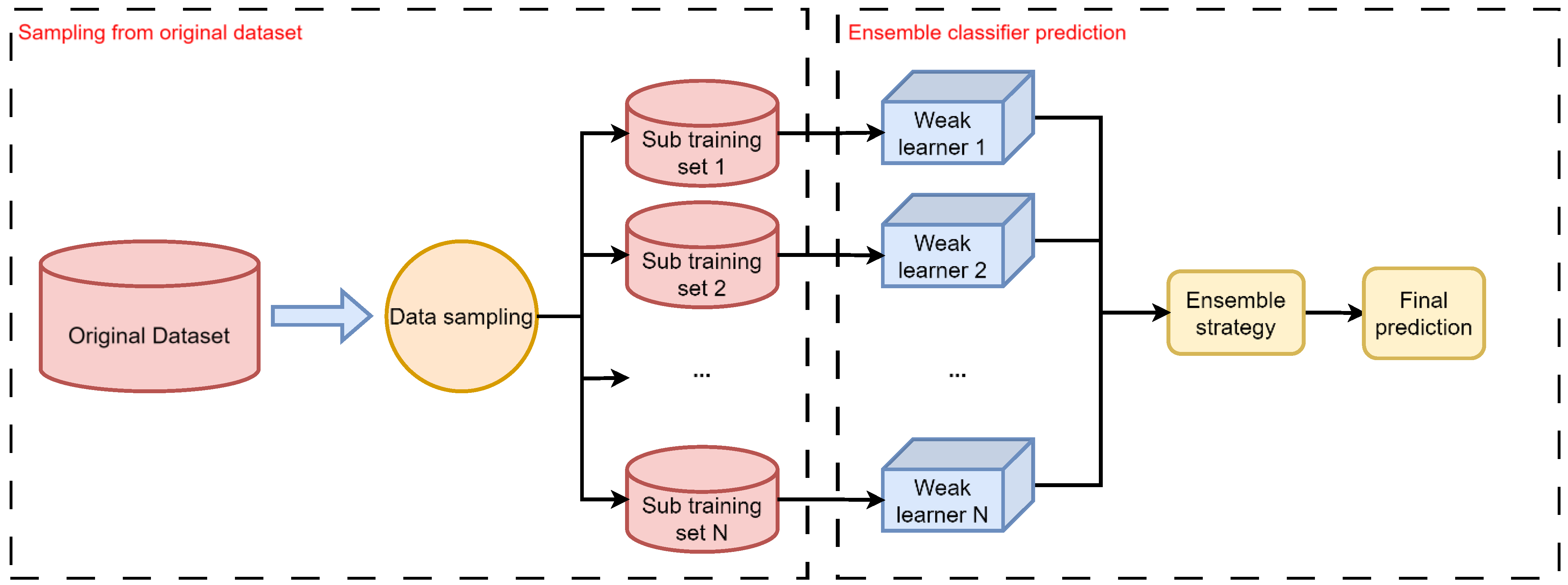
Ensemble learning methods have been proved to be an efficient way to deal with class imbalance and bagging is one of those ensemble learning methods that is widely used and easy to realize. By training a set of weak classifiers based on different sub-datasets, a strong classifier can be obtained by combining their predictions together. Figure 2 illustrates the main process of bagging. Specific information about the bagging framework can be described as follows.

Generating sub-datasets. The first stage of building a bagging classifier is to generate a set of sub-datasets by random sampling. In this process, it should be confirmed how many samples should be taken out of the base datasets and how many sub-datasets should be generated. Usually, these two parameters can be confirmed by expert knowledge or by cross validation.

Training weak classifiers. After generating the sub-datasets, the training process can be started. Each sub-dataset corresponds to a weak classifier and each weak learner is built by corresponding sub-datasets. Because every sub-dataset is generated by random sampling, the weak learners are independent theoretically.

Combining output results. Once the weak learners have completed their classification results, respectively, it is necessary to combine these outputs to obtain a final result. There are several strategies to achieve combination. (i) Voting. By counting all the classification results, the most voted class is the final result. (ii) Weighted averaging. Differently from the voting method, this method sets a weight for each weak learner. With a greater weight, a weak learner is more important compared to others. In this paper, the voting strategy is used as the combination method.

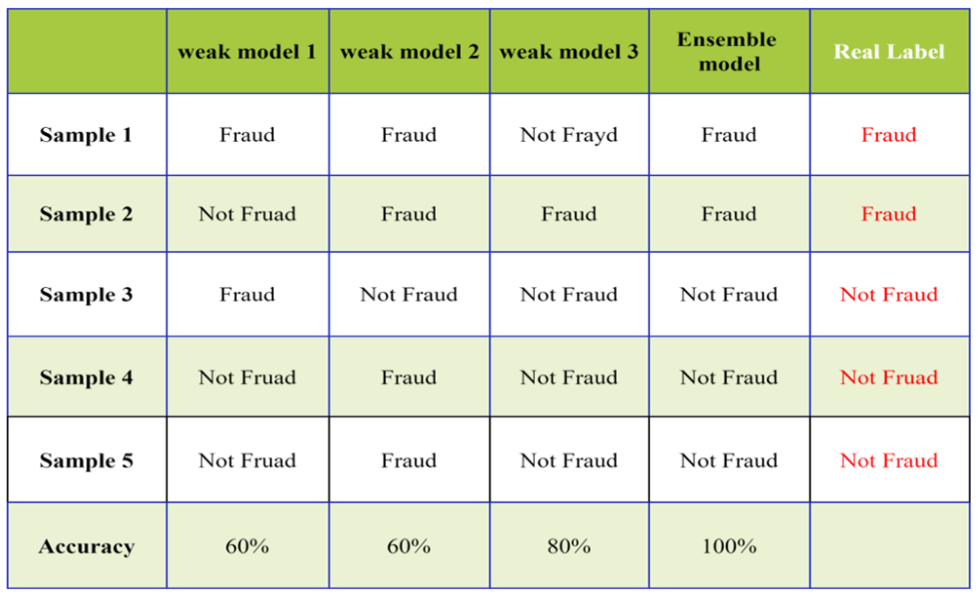
Ensemble learning is an excellent approach for improving model performance. However, when implementing ensemble methods, two key factors must be considered, diversity among weak classifiers and a reasonable level of individual accuracy.

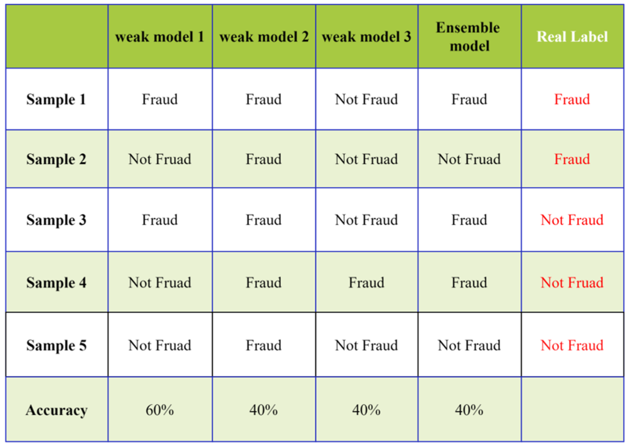
As shown in Figure 3, when each weak classifier has a reasonable performance and the classification results differ across samples, the final ensemble effect can be highly effective. However, as illustrated in Figure 4, when each weak classifier performs poorly, the final results of the ensemble model can be worse.

3.4. Feature Selection

In fraud detection datasets, there are typically numerous attributes, but not all of them are equally relevant for the targeted task. For instance, certain attributes such as transaction amount and user age prove to be critical in detecting fraudulent transactions as abnormal transaction amounts suggest fraudulent behavior and some age groups are more susceptible to becoming targets of fraud. Conversely, attributes like user gender and transaction time may be less important for fraud detection. Therefore, selecting the most important attributes is a crucial step as it can significantly reduce the complexity of the model. Especially for BRB models, it helps avoid the combinatorial explosion problem during the BRB modeling process.

In this work, XGBoost feature importance analysis is adopted as the feature selection method. Extreme gradient boosting [47] is an optimized gradient boosting implementation that is known for its efficiency, flexibility and state-of-the-art performance in many machine learning problems, such as classification and regression. During the past decades, it has become a widely used and highly effective machine learning tool. In this section, the mechanism of how XGBoost is used as a feature selection technique is briefly introduced as follows.

The XGBoost algorithm is an ensemble learning method composed of decision trees. Take a dataset with input samples set at $X=\{x_1,x_2,\dots ,x_n\}$ and corresponding labels set at $Y=\{y_1,y_2,\dots ,y_n\}$. The dataset can be described as $DS=\left\{\left(x_i,y_i\right):i=1\dots n,x_i\in {\mathbb{R}}^M,y_i\in \mathbb{R}\right\}$. The output of XGBoost ${\widehat{y}}_i$ is defined as follows.

$${\widehat{y}}_i={\displaystyle \sum _{k=1}^K{f}_k(x_i),f_k\in F}$$

(9)

where ${\widehat{y}}_i$ is the prediction value of input sample $x_i$. $f_k$ denotes the k-th decision tree in the tree space $F$. $F=\{f_1,f_2,\dots ,f_K,\}$, where $f_k:X\to \mathbb{R}$, and K is the total number of decision trees. The objective function $Obj:\mathbb{R}\times Y\to \mathbb{R}$ is described in Equation (9). The goal is to minimize the function $Obj$ in Equation (10).

$$Obj={\displaystyle \sum _{i=1}^{n}l}\left({\widehat{y}}_i,y_i\right)+{\displaystyle \sum _{k=1}^K\Omega }\left(f_k\right)$$

(10)

where $l\left({\widehat{y}}_i,y_i\right)$ is the loss between the i-th input sample’s prediction value and real value and $\Omega :F\to \mathbb{R}$ denotes the penalty parameters which is used for controlling the complexity of the decision tree in order to avoid overfitting. In the XGBoost algorithm, each decision tree is generated iteratively and the t-th decision tree is created based on fitting the loss between the sum of the outputs of the existing decision trees in the (t − 1)-th iteration and the true values. In this process, the goal is to minimize the function $L^{(t)}$, which is illustrated in Equation (11)

$$L^{(t)}={\displaystyle \sum _{i=1}^n\left[l\left(y_i,{\widehat{y}}_i^{t-1}+f_t(x_i)\right)\right]}+\Omega \left(f_t\right)$$

(11)

where ${\widehat{y}}_i^{t-1}$ denotes the sum of existing decision trees’ prediction of the i-th instance at the (t − 1)-th iteration.

Each tree in XGBoost consists of several nodes and each node selects the attribute with the highest information gain at the current position from all the available attributes to serve as the node. XGBoost typically measures the importance of each attribute by calculating its information gain, which is then used for feature selection. First, calculating the number of times each attribute serves as a node across all trees.

$$Weight(featur{e}_i)={\displaystyle \sum _{k=1}^{K}Coun{t}_k(featur{e}_i)}$$

(12)

where $Weight(featur{e}_i)$ denotes the number of times the i-th attribute serves as a node across all trees. $Coun{t}_k$ is the times the i-th attribute serves as a node in the k-th tree. After calculating the formula above, the next step is to calculate the average information gain of each attribute. The calculation formula is as follows.

$$Gain(featur{e}_i)={\displaystyle \frac{1}{Weight(featur{e}_i)}}{\displaystyle \sum _{k=1}^K{\displaystyle \sum _{n\in Node{s}_k(featur{e}_i)}Gai{n}_n}}$$

(13)

where $Gain(featur{e}_i)$ denotes the average information gain of the i-th attribute and $Node{s}_k(featur{e}_i)$ denotes the set of all the nodes in the k-th tree that use the i-th feature. $Gai{n}_n$ is the information gain when node n uses the i-th attribute. The greater the average information gain of an attribute, the more important the attribute is.

4. Constructions of Ensemble BRB

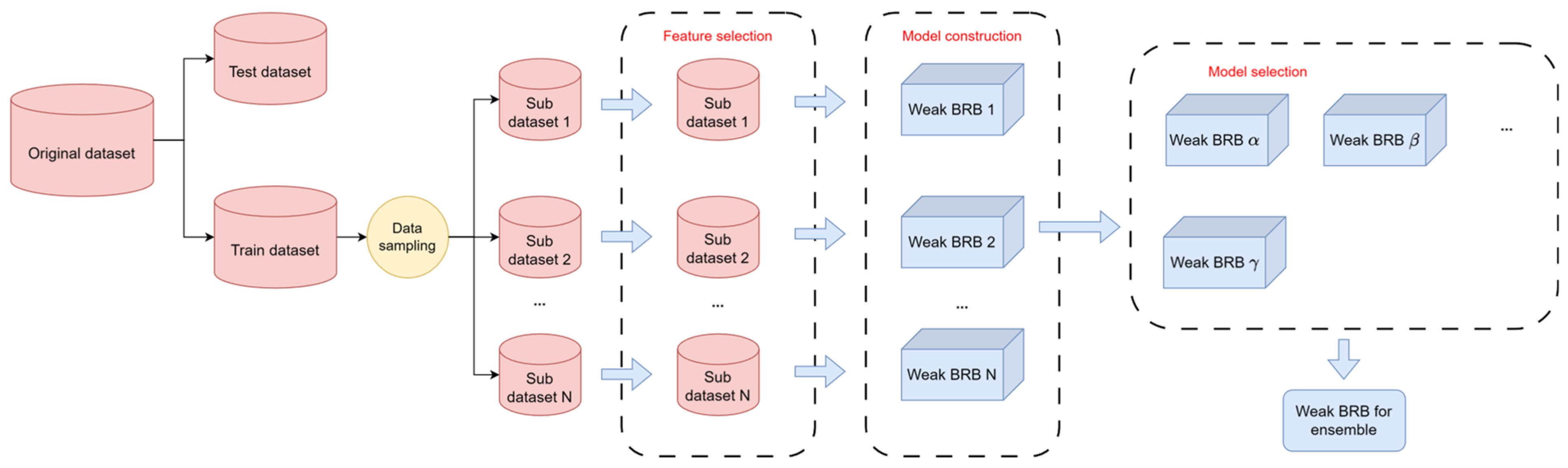
In this section, the main process of constructing ensemble belief rule base model is shown. In Figure 5, the modeling process of the ensemble BRB has been divided into five steps. Each modeling step can be described as follows.

Step 1. Data sampling.

This process involved two rounds of data sampling. The first round was used to split the original dataset into the training dataset and test dataset. After that, a novel data sampling strategy was used to generate the sub-datasets used for generating the weak classifiers (i.e., the weak BRB model). It is important to note that the dataset used in the experiment was large and extremely imbalanced. Therefore, the sampling needed to be carefully balanced to ensure sample diversity while retaining as much information as possible. In this study, for the non-fraudulent data, approximately 60% to 70% of the total samples were extracted, while all the fraudulent data were included in the training process. The sampling process can be described as follows.

In a given dataset, $DS=\{P,N\}$, $P=\{x_1^{+},x_2^{+},\dots ,x_{n+}^{+},\}$ is the set of positive samples and $N=\{x_1^{-},x_2^{-},\dots ,x_{n-}^{-},\}$ is the set of negative samples.

$${N^{\prime }}_i=Sampling(N,\gamma ),\gamma \in (0,1]$$

(14)

$$D{S^{\prime }}_i=P\cup N^{\prime }$$

(15)

where $\gamma$ denotes the ratio of data sampling, ${N^{\prime }}_i$ is the i-th set of negative samples after data sampling and ${{DS}^{\prime }}_i$ is the i-th dataset after data sampling.

Step 2. Feature selection.

In this step, feature selection was performed on the data subsets generated in the previous step. Here, we used the XGBoost feature selection method to select features from the generated data subsets. By applying feature selection in the process of the weak BRBs’ construction, the combinatorial explosion problem can be avoided and each BRB’s performance can be ensured. The feature selection process can be described as in Equation (16).

$$\{x_{\alpha ,i},x_{\beta ,i}\}=XGBoostFS({{DS}^{\prime }}_i)$$

(16)

where $x_{\alpha ,i},x_{\beta ,i}$ denotes the selected two features of ${{DS}^{\prime }}_i$ and $XGBoostFS$ means the method of feature selection based on XGBoost feature importance analysis.

Step 3. BRB construction.

In this step, based on the generated dataset and the selected attributes, the construction process of the weak BRBs can begin. This process involved steps such as referential value setting, initial confidence rule construction, parameter optimization and so on. The process of BRB construction can be described as in Equation (17).

$$\begin{array}{l}wBR{B}_i=model(x_{\alpha ,i},x_{\beta ,i},Para{m}_i,CMA-ES)\\ i=1,2,\dots ,num\end{array}$$

(17)

where $wBR{B}_i$ denotes the i-th weak BRB model, $model$ is the construction process of BRB and $num$ is the number of weak BRB models. $Para{m}_i$ means the parameters used for i-th BRB construction such as referential values of attributes, referential values of output, weight of attributes and weights of rules. $CMA-ES$ denotes the CMA-ES algorithm (Covariance Matrix Adaptation–Evolution Strategy) used for the parameter optimization.

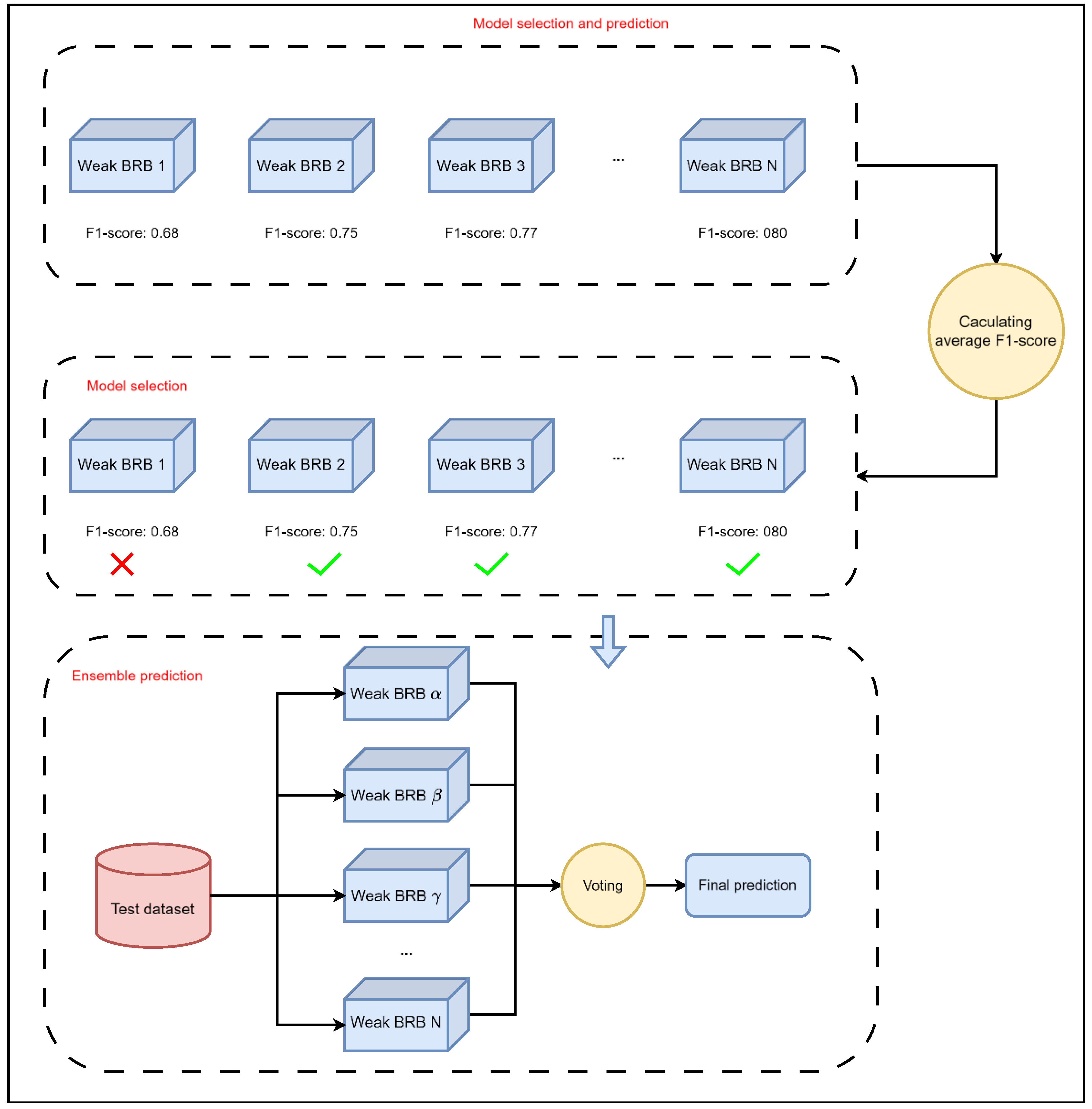
Step 4. Model selection.

In the previous step, each weak BRB model will produce a prediction result. In this phase, the trained models were tested and filtered because the sampling was random, so it could not guarantee that every generated model would be useful. Since ensemble learning frameworks can only achieve the best performance when each model has a certain level of accuracy and is independent, it was crucial to filter out and select the models with adequate accuracy.

Step 5. Combining weak BRBs.

Finally, all the weak BRB classifiers were added to the ensemble by adopting the majority voting strategy. After the ensemble, the entire modeling process for the integrated BRB was completed. The process of voting strategy can be described as in Equation (18).

$$Prediction=\left({\displaystyle \sum _{i=1}^{num}{O}_i}\right)/num$$

(18)

where $Prediction$ means the average prediction value after combining each weak BRB model and $O_i$ denotes the prediction value of i-th weak BRB model. If $Prediction$ is less than 0.5, the final prediction of the ensemble BRB model is negative. Otherwise, the final prediction is positive.

For the specific modeling steps, please refer to Figure 5, Figure 6 and Figure 7.

In this ensemble BRB framework, we have made improvements to the traditional bagging ensemble framework. Firstly, unlike the traditional random bootstrap method in the data sampling process, we only apply random sampling to the major class samples, while preserving all the minor class samples. This approach has the advantage of mitigating the effects of sample imbalance to some extent in the generated dataset after sampling, while retaining as much information as possible from the minor class samples. Additionally, we also control the sampling ratio, setting it at 60% to 70% of the original major class samples. A sampling ratio that is too large results in a lack of diversity between data subsets, while one that is too small risks losing important information. Maintaining this ratio effectively balances the diversity and performance of the weak BRB ensemble.

In traditional ensemble frameworks, decision trees are commonly used as base classifiers. The construction process of decision trees involves feature selection, namely node selection, which includes the process of randomly generating feature subsets during data sampling to increase model diversity. However, in ensemble frameworks based on the BRB model, there is no feature selection process. If we simply adopt the traditional bagging framework’s approach of randomly generating feature subsets, it will significantly affect the performance of weak classifiers. Therefore, for this step, we introduce a feature selection process. After generating data subsets, we use XGBoost feature importance analysis to select features for the data subsets and then model weak BRBs based on the selected attributes. This approach significantly enhances the model performance of weak BRBs, further improving the overall model effectiveness after ensemble. At the same time, by applying the feature selection method, the combinatorial explosion problem during the modeling process can be avoided.

5. Experimental Study

5.1. Dataset Information

In this section, two datasets from the Kaggle competition of credit card fraud detection is used to validate the effectiveness of our method. Dataset #1 “https://www.kaggle.com/datasets/mlg-ulb/creditcardfraud (accessed on 11 July 2023)” is widely used in fraud detection research. To further validate the effectiveness of our method on multiple datasets, we also conducted experiments on Dataset #2 “https://www.kaggle.com/datasets/nelgiriyewithana/credit-card-fraud-detection-dataset-2023 (accessed on 10 January 2025)”. Dataset #2 is very recent, collected in 2023 from European cardholders. Both datasets have been anonymized to protect users’ personal information. The basic information of these two datasets is shown in

Table 1. Summary of fraud detection datasets.

Dataset	Size	Distribution	Imbalance Ratio	#Attributes
Dataset #1	284,807	284,315/492	577.88	30
Dataset #2	568,630	284,315/284,315	1	29

.

From Table 1 we can find out that both Dataset #1 and Dataset #2 are extremely large. The number of samples in Dataset #1 exceeds 280,000, while the number of samples in Dataset 2 surpasses 560,000. Also, there are only 492 instances of fraud samples in Dataset #1. Therefore, there is an extreme class imbalance between these two classes. The imbalance ratio can reach more than 500. Also, the numbers of attributes in both datasets are 30 and 29, respectively, which is also very large for constructing a BRB model.

5.2. Evaluation Matrices

To avoid the impact of data imbalance and comprehensively consider the accuracy and completeness of the model, the experimental results are evaluated in the form of F1 score, precision and recall, which can be described as in Equation (19) to Equation (22).

$$F1\hspace{0.17em}\hspace{0.17em}score={\displaystyle \frac{2\times Recall\times Precision}{Recall+Precision}}$$

(19)

where F1 score is the hybrid indicator of the recall and precision of a classifier; the formulas of accuracy, precision and recall are shown as follows.

$$Accuracy={\displaystyle \frac{TP+TN}{TP+FP+TN+FN}}$$

(20)

$$Precision={\displaystyle \frac{TP}{TP+FP}}$$

(21)

$$Recall={\displaystyle \frac{TP}{TP+FN}}$$

(22)

where TP (True Positive), FN (False Negative), FP (False Positive) and TN (True Negative) are the four indicators obtained from a confusion matrix, as shown in

Table 2. Definition of confusion matrix.

	Predicted Positive	Predicted Negative
Actual Positive	TP	FN
Actual Negative	FP	TN

. TP is the number of instances where the model correctly predicted the positive class. FN is the number of instances where the model incorrectly predicted the negative class, while the actual class was positive. FP is the number of instances where the model incorrectly predicted the positive class, while the actual class was negative. TN is the number of instances where the model correctly predicted the negative class.

In fraud detection, our primary concern is how well the model performs when facing the challenge of extreme class imbalance. Utilizing multiple evaluation metrics allows a more comprehensive and objective assessment of the model’s performance. Among these, accuracy is used to measure the overall accuracy of the model. However, due to the significant class imbalance in the dataset, this metric often fails to differentiate between models effectively. Therefore, the F1 score and recall on minority class are more indicative of the model’s comprehensive performance.

In credit card fraud detection, the data used for model construction are crucial, as biases in data may exist. Therefore, it is essential to select a large-scale dataset to cover as many scenarios as possible. Additionally, using multiple datasets can help better validate the model’s effectiveness and generalization capability. Furthermore, unintended consequences of model deployment should also be discussed. In real-world scenarios, the number of fraud samples is significantly smaller than that of normal samples, making data imbalance a persistent challenge in fraud detection. The key lies in accurately identifying fraud samples. If the model fails to achieve this, unintended consequences may arise, such as misclassifying normal samples as fraud or overlooking fraud samples. The former leads to wasted resources, while the latter leaves potential risks. Therefore, the ability to accurately detect fraud samples is of paramount importance.

5.3. Modeling Steps and Classification Results of Ensemble BRB

This section presents several weak BRBs’ results after model selection to demonstrate the experimental effectiveness of the corresponding steps.

Step 1. Data sampling.

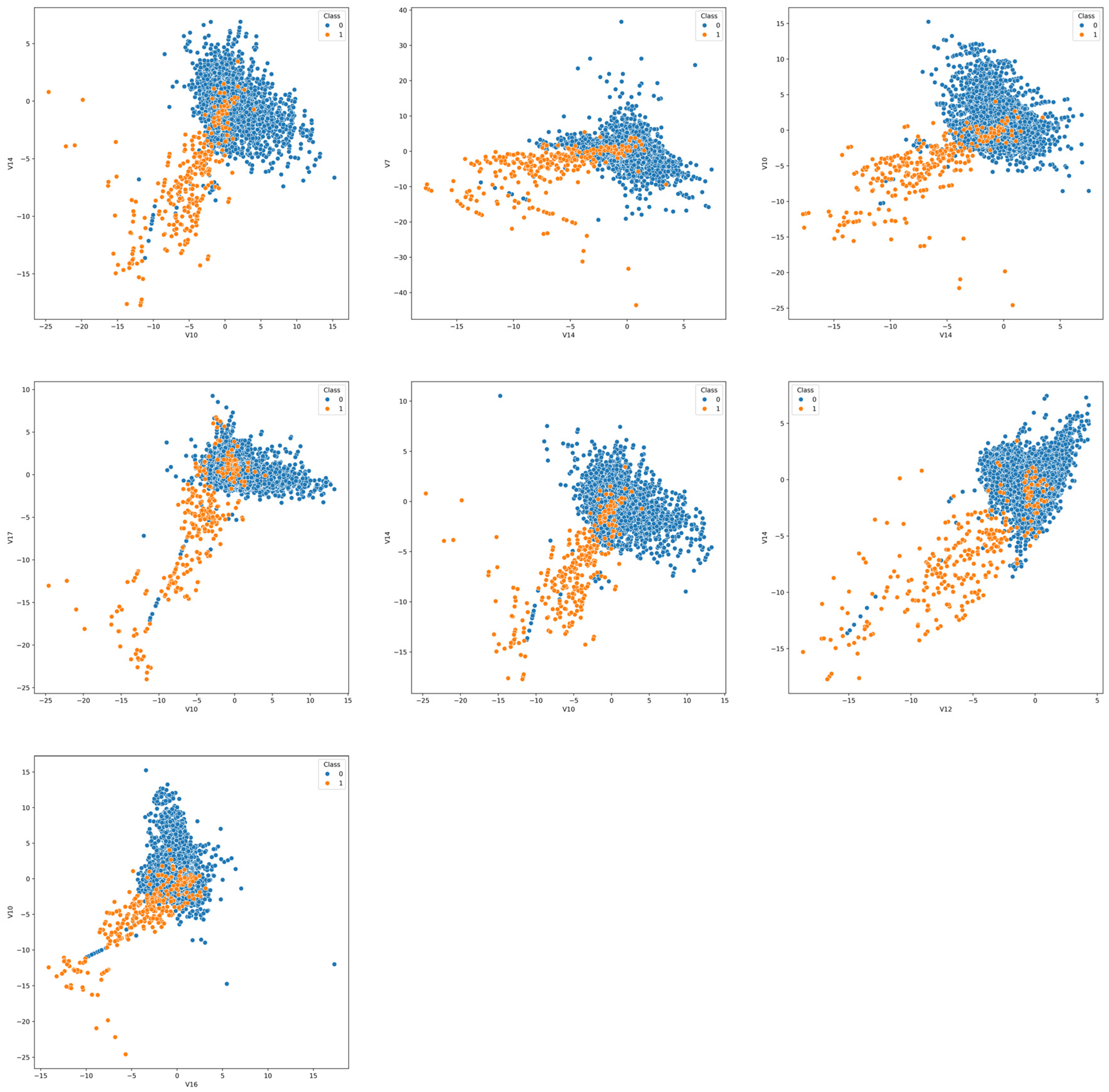
As mentioned in Section 4, for this fraud detection task, we employed an innovative data sampling approach. We retained all the samples of fraud transactions in the dataset and only conducted bootstrap sampling on the normal transaction samples. The results after the data sampling of Dataset #1 are illustrated in Figure 8.

Step 2. Feature selection.

During the feature selection process, we employed the XGBoost feature importance analysis method to filter the most important two features of these two datasets. The example results of feature selection in Dataset #1 are presented in

Table 3. Feature selection results of weak BRBs in Dataset #1.

Dataset	Feature 1	Feature 2
Sub-dataset 1	V10	V14
Sub-dataset 2	V14	V7
Sub-dataset 3	V14	V10
Sub-dataset 4	V10	V17
Sub-dataset 5	V10	V14
Sub-dataset 6	V12	V14
Sub-dataset 7	V16	V10

.

Due to the sensitive nature of the dataset, the attributes are presented in an anonymized form, possibly representing processed transaction timestamps, dates and other features. The feature selection results reveal certain characteristics—the selected features demonstrate diversity, while some features like V14 and V10 appear with notably higher frequency than others. This result is reasonable since one of the most important aspects of ensemble learning is achieving a balance between diversity and performance. When the sampling rate is too high, there is excessive overlap between different datasets, resulting in a loss of diversity. Consequently, the attributes selected from each dataset are likely to be identical, meaning that these weak BRBs would likely produce similar outputs for the same sample, defeating the purpose of ensemble learning. Conversely, if the sampling rate is too low, too much information is lost, leading to the poor performance of individual weak BRBs, which also results in unsatisfactory ensemble results. Figure 3 and Figure 4 illustrate this point with a simple example.

Step 3. Construction of weak BRBs.

Based on the sub-dataset after feature selection in Step 2, the weak BRBs are constructed. The construction process of each weak BRB typically includes initial parameter settings, primarily involving the initialization of belief distribution, attribute weights, rule weights, etc. These parameters are usually determined based on expert knowledge. In the absence of specific research, attribute weights and rule weights are typically set to 1.

The classification results of the weak BRBs after construction are shown in

Table 4. Performance of weak BRBs and ensemble BRB in Dataset #1.

Model	F1 Score	Accuracy	Recall
Sub_BRB_1	0.7911	0.9993	0.7435
Sub_BRB_2	0.8208	0.9994	0.8272
Sub_BRB_3	0.8010	0.9993	0.8010
Sub_BRB_4	0.7680	0.9992	0.7539
Sub_BRB_5	0.7649	0.9993	0.7068
Sub_BRB_6	0.7810	0.9993	0.7749
Sub_BRB_7	0.7766	0.9992	0.8010
Ensemble BRB	0.8375	0.9995	0.8978

and

Table 5. Performance of weak BRBs and ensemble BRB in Dataset #2.

Model	F1 Score	Accuracy	Recall
Sub_BRB_1	0.9527	0.9633	0.9372
Sub_BRB_2	0.9532	0.9673	0.9230
Sub_BRB_3	0.9485	0.9688	0.9142
Sub_BRB_4	0.9095	0.9230	0.8872
Sub_BRB_5	0.9264	0.9441	0.9102
Sub_BRB_6	0.9126	0.9301	0.9223
Sub_BRB_7	0.9448	0.9724	0.9401
Ensemble BRB	0.9950	0.9973	0.9952

.

Step 4. Model selection.

After step 3, multiple weak BRBs are constructed. Since there is a degree of randomness involved in building weak BRBs, a model selection process is required for all the weak BRBs. Based on their performance in the test set, such as their F1 score, the models with relatively good scores are selected to proceed to the next step.

Step 5. Combining weak BRBs.

After selecting the weak BRBs in step 4, their outputs are combined. In this paper, we employ a voting method to combine the outputs of the weak BRBs.

As can be seen from Figure 8, the data sampled using the improved sampling method exhibit a lower degree of imbalance while still preserving most of the original data distribution characteristics. Moreover, according to the feature selection results shown in Table 3, the sampled data exhibit the following two main features. (1) Different weak BRBs select different features. (2) Some features appear more frequently than others. These two points indicate that the improved sampling method reaches a balance between diversity and performance. Excessively random feature selection would degrade the classification performance of the weak classifiers, while overly similar feature selection would fail to maintain the diversity required for effective ensemble learning.

As shown in Table 4 and Table 5, the performances of selected weak BRB models in the test set vary, but after the model selection process, most of the metric values fall within a stable range. For instance, in Dataset #1, the F1 scores are concentrated between 0.76 and 0.82. By combining the outputs of all the weak BRBs, the ensemble BRB achieves the optimal performance across all the metrics reported in the table, demonstrating the effectiveness of the innovative ensemble method proposed in this paper for BRB models.

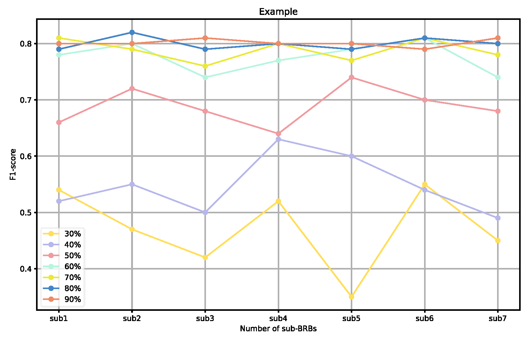
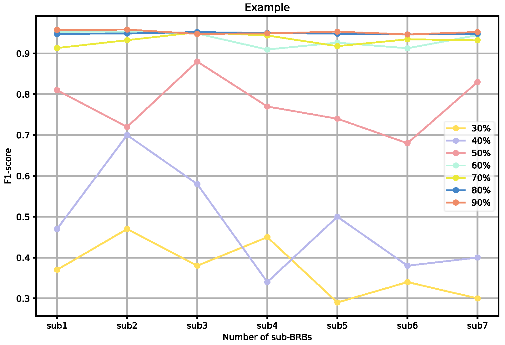
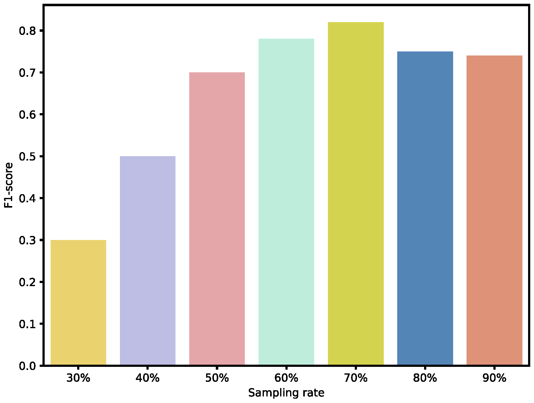
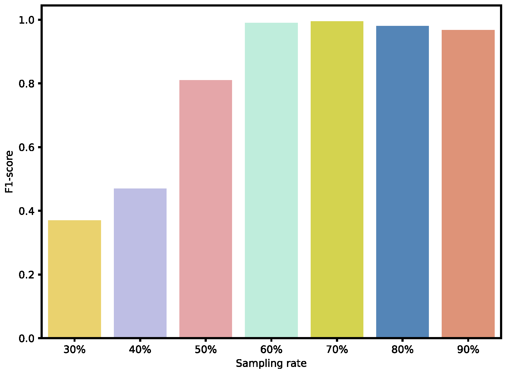
To further validate the effectiveness of our sampling ratios, we also analyzed the performance of individual weak BRBs classified under different sampling ratios, as well as the overall ensemble performance. As shown in Figure 9 and Figure 10, when the sampling ratio is below 50%, the performance of the weak BRB classifiers is highly variable and generally poor, and the ensemble performance is also suboptimal. As the sampling ratio increases, the performance of the weak classifiers gradually improves, stabilizing when the ratio exceeds 70% Additionally, as shown in Figure 11 and Figure 12, although the performance of individual weak classifiers approaches optimal levels when the sampling ratio reaches 80% or 90%, the ensemble model’s performance is actually lower than that of the ensemble model with a 60–70% sampling ratio. This is because, at very high sampling ratios, the classifiers lack diversity, making ensemble learning less effective. In contrast, with a 60–70% sampling ratio, the weak classifiers maintain both diversity and individual performance, resulting in the optimal ensemble model at this level. Additionally, ensemble size is a key factor affecting the ensemble performance. As the number of ensemble members increases, the performance of the ensemble model gradually improves. However, after reaching a critical point, additional ensemble members become meaningless and do not further improve the model’s performance. In the experiments on both datasets, we selected an ensemble size of seven, as performance improvements became insignificant when exceeding this number.

5.4. Complexity Improvements

In this section, we will present the improvements made by the proposed ensemble BRB method over traditional BRB models in terms of model complexity, using mathematical formulations.

The complexity of a BRB model is primarily determined by the number of rules it contains. In this case, we compare the complexities of the proposed ensemble BRB model and the traditional BRB model by calculating their respective numbers of rules.

Given a dataset with $M$ attributes, where i-th attribute has $A_i$ referential values, the number of rules $n\_rules$ in a traditional BRB model can be calculated using Equation (23) as follows.

$$n\_rules={\displaystyle \prod _{i=1}^M{A}_i}$$

(23)

In the method proposed in this paper, the number of rules is calculated as shown in Equation (24).

$$n\_rules=n\times {\displaystyle \prod _{i=1}^2{A}_i}$$

(24)

where $n$ represents the number of weak BRBs in the ensemble BRB.

Plugging in the values from the fraud detection dataset used in this paper, where $M$ is 30, $A_i$ is 4 uniformly and $n$ is 7, the complexities of the two models are calculated as follows.

The number of rules of the traditional BRB is $4^{30}$, while the number of rules of the ensemble BRB is $7\times 4^2=112$. It can be seen that in building the traditional BRB model, the combinatorial explosion problem arising from the large number of attributes in the fraud detection dataset makes it difficult to construct the model. On the other hand, the proposed method of combining the ensemble BRB with feature selection can effectively avoid the combinatorial explosion problem, reducing the modeling difficulty of BRB models when dealing with high-dimensional data.

5.5. Comparative Research

In comparative experiments, we chose several classic classifiers to conduct a comparative study of the ensemble BRB classifier which includes support vector machine, decision tree, K-Nearest Neighbors, logistic regression, bagging tree and boosting tree (Adaboost). We split the original dataset into a training dataset and test dataset with a ratio of 6 to 4. Also, we conducted experiments combining the BRB model with common methods for handling imbalanced classification problems (SMOTE and cost-sensitive learning). The experimental results are shown in Figure 13 and Figure 14, and

Table 6. Classification results of comparative research in Dataset #1.

Model	F1 Score	Accuracy	Recall
SVM	0.8164	0.9994	0.7435
Decision Tree	0.7714	0.9993	0.8272
KNN	0.7966	0.9994	0.8010
LR	0.7245	0.9992	0.7539
Bagging Tree	0.8232	0.9995	0.7068
Boosting Tree	0.8176	0.9995	0.7749
BRB	\	\	\
BRB + FS	0.7395	0.9991	0.7801
BRB + FS + SMOTE	0.7852	0.9992	0.8325
BRB + FS + CS learning	0.8060	0.9993	0.8482
Our method	0.8375	0.9995	0.8978

and

Table 7. Classification results of comparative research in Dataset #2.

Model	F1 Score	Accuracy	Recall
SVM	0.9567	0.9579	0.9325
Decision Tree	0.9970	0.9970	0.9984
KNN	0.9392	0.9334	0.8901
LR	0.9546	0.9557	0.9334
Bagging Tree	0.9998	0.9998	1.0000
Boosting Tree	0.9989	0.9991	0.9992
BRB	\	\	\
BRB + FS	0.9556	0.9591	0.9284
Our method	0.9950	0.9973	0.9952

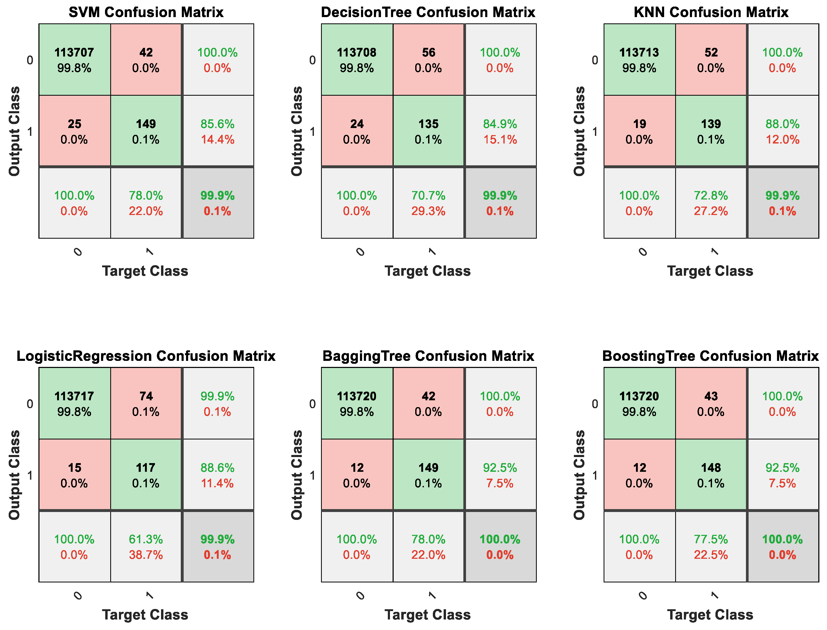
. In Table 5, “FS” means “Feature Selection” and “CS” means “Cost Sensitive”. Figure 13 and Figure 14 are confusion matrices used to evaluate the classification performance of the model. In these figures, “Output class” represents the model’s predicted results, while “Target Class” represents the true labels of the samples. “0” denotes “Not Fraud” and “1” denotes “Fraud”. In Figure 13 and Figure 14, the squares with green backgrounds represent correctly classified examples, while the squares with red backgrounds represent incorrectly classified examples. These two figures provide insight into the detailed classification results of the model.

As shown in Table 5 and Table 6, multiple evaluation metrics were utilized to assess the classification performance of the classifiers in this study. Specifically, the confusion matrix was used to observe the detailed classification outcomes, the F1 score was used to evaluate the overall performance and the recall was used to measure the performance in the minor class. After all, for experiments in this study, the algorithm’s performance in the minor class is of greater concern. Therefore, compared to accuracy, the recall and F1 score are more representative.

For Dataset #1, based on the data presented in Table 6, it can be observed that the accuracy scores of various classifiers do not exhibit significant differences overall. This is because the dataset has a very high class imbalance, so the performance in the main class plays a decisive role in determining the overall accuracy. Hence, in order to accurately assess the effectiveness of these classifiers, it is important to evaluate their performance specifically in the minor class. Table 5 shows that our method ranks at the top for all three metrics. It achieves the highest F1 score, accuracy and recall, which is a remarkable performance. These results confirm the effectiveness of our method in imbalanced datasets and demonstrate that it is competitive with traditional machine learning classifiers for the fraud detection task. In contrast, some classifiers, notably SVM, are negatively affected by the data imbalance, resulting in low recall. Furthermore, our method offers better interpretability compared to other classifiers. The results show that a standard BRB model is unable to handle the fraud detection task effectively. With as many as 30 attributes, the BRB model faces a combinatorial explosion problem that makes modeling impossible. Therefore, attribute dimensionality reduction is essential. Additionally, our method demonstrates significant improvements when compared to approaches that combine BRB with SMOTE or cost-sensitive learning. Although combining the BRB model with SMOTE or cost-sensitive learning methods can improve its performance in minority class samples, the enhancement is limited due to inherent drawbacks in these approaches. SMOTE tends to cause overfitting, while cost-sensitive learning methods struggle with determining optimal parameters.

For Dataset #2, according to Table 7, although our method did not achieve the best performance across all the metrics, we can see that its performance is close to that of the best-performing bagging tree. Moreover, Dataset #2 is not an imbalanced dataset, and the comparison between these two datasets better demonstrates the effectiveness of our method in real-world imbalanced scenarios. Additionally, testing on multiple datasets demonstrates our model’s generalization capability.

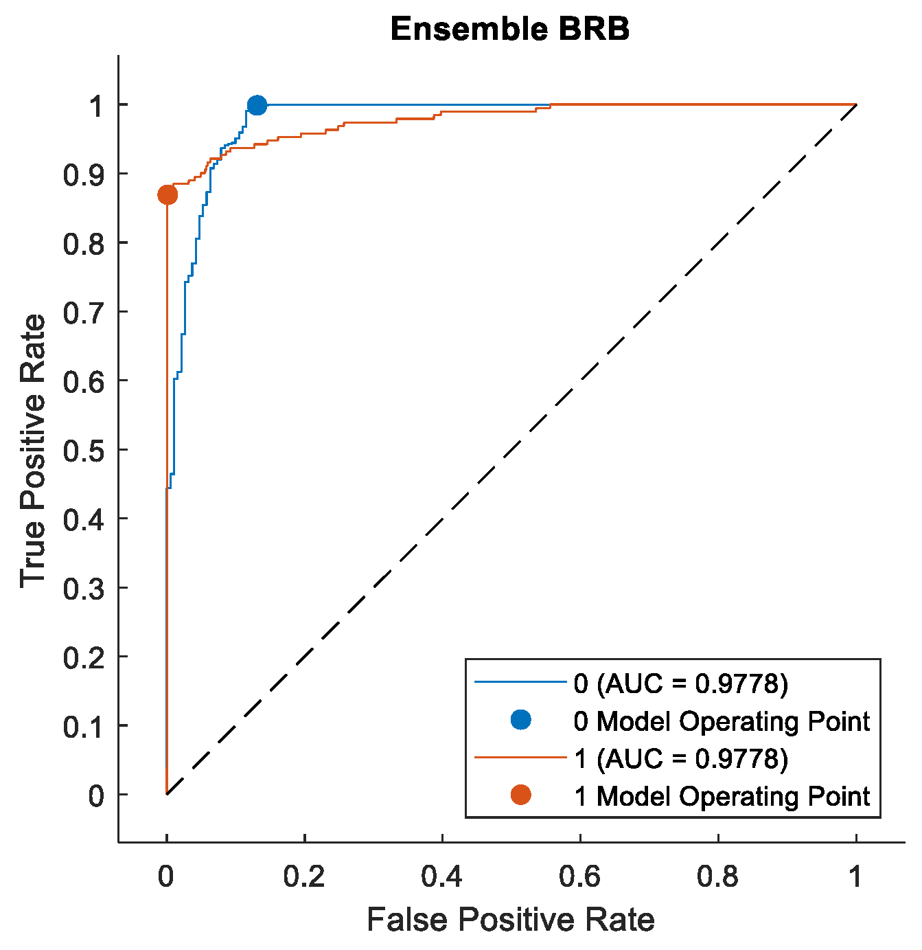
To further validate the effectiveness of our method on the fraud detection task, we plotted the Receiver Operating Characteristic (ROC) curves for the classification results of various models, as shown in Figure 15 and Figure 16. The ROC curve is an important metric for evaluating the performance of binary classification tasks, as it comprehensively reflects the overall performance of a classifier. The area under the ROC curve (AUC) provides a comprehensive assessment of a classifier’s quality. The ROC curve visually illustrates the trade-off between sensitivity and specificity at different threshold settings, aiding in the selection of an appropriate threshold to balance false positives and false negatives. Moreover, the ROC curve is not influenced by the prior probability distribution of the data, making it effective even for imbalanced datasets, rendering it highly suitable for evaluating classification tasks in practical scenarios. These characteristics have led to the widespread application of ROC curves in fields such as machine learning and data mining.

From these two figures, we can observe that ensemble BRB method achieved the highest AUC value of 0.9788. The bagging tree and boosting tree methods closely followed, with both methods exhibiting nearly identical performance, reaching an AUC of 0.9691. Due to the inherent characteristics of the KNN and decision tree algorithms, their predictions cannot typically be transformed into probability distributions. Consequently, their ROC curves exhibit a two-segment linear form. A larger AUC value indicates that the ensemble BRB model exhibits superior classification capabilities compared to the other models.

The above experiments demonstrate that the proposed method exhibits good performance. However, there are also some limitations. First, while the large scale of the dataset used in the experiments reflects the potential of the proposed method in this field, the challenges posed by the massive scale of real-time credit card transaction data in practical applications warrant further investigation. Human in the Loop (HITL) [48] is an approach in machine learning and artificial intelligence that integrates human input into the training, decision-making, or refinement process of algorithms. It leverages human expertise to address model weaknesses, correct errors and improve system performance. For future work, we plan to integrate the HITL method with our approach. We think such integration would allow domain experts to periodically validate and refine the rule base, particularly focusing on boundary cases and anomalies in the data streams. This selective human intervention could help maintain decision quality while managing computational costs as data volumes grow. Additionally, there are certain limitations regarding input data characteristics in the method proposed in this paper. While the introduction of feature selection has reduced the modeling complexity, credit card transaction data often suffers from missing values. In cases where a sample lacks the attributes corresponding to the model, it becomes difficult for the model to make predictions. Therefore, this model has specific requirements for input data quality, which is an area worthy of future improvement. Enhancing this aspect would help improve the model’s applicability.

6. Conclusions

In this study, we proposed a novel ensemble BRB model to predict fraud detection. Compared to the traditional ensemble learning framework, we made several improvements as follows:

• When generating data subsets through random sampling, we retained all fraud samples and performed sampling only on normal samples;
• The feature selection process is added the model construction;
• The model selection process is added to the model construction.

With these improvements, the ensemble BRB model can better handle fraud detection problems. The experimental results demonstrate that the ensemble BRB achieves optimal performance across multiple evaluation metrics in Dataset #1. In Dataset #2, the ensemble BRB achieved a performance comparable to the best-performing model. Also, by using BRB as the base classifier, the ensemble model gains enhanced interpretability. The model proposed in this paper focuses on addressing the imbalanced classification and interpretability issues in credit card fraud detection tasks. By combining the ensemble learning framework with the BRB model, we enhanced the model’s interpretability, making the decision-making process more transparent. For instance, when a transaction is predicted as fraudulent, the prediction process can be traced through the BRB’s principle formulas, a feature that helps financial institutions and customers understand the basis for decisions, thereby increasing trust in the system. Additionally, data imbalance often leads to high false positive rates in fraud detection systems, which the ensemble learning framework effectively mitigates. This not only reduces the inconvenience caused to customers and merchants by false alarms but also strengthens financial institutions’ confidence in the detection results.