A Refined Approach to Segmenting and Quantifying Inter-Fracture Spaces in Facial Bone CT Imaging

Abstract

The human facial bone is made up of many complex structures, which makes it challenging to accurately analyze fractures. To address this, we developed advanced image analysis software which segments and quantifies spaces between fractured bones in facial CT images at the pixel level. This study used 3D CT scans from 1766 patients who had facial bone fractures at a university hospital between 2014 and 2020. Our solution included a segmentation model which focuses on identifying the gaps created by facial bone fractures. However, training this model required costly pixel-level annotations. To overcome this, we used a stepwise annotation approach. First, clinical specialists marked the bounding boxes of fracture areas. Next, trained specialists created the initial pixel-level unrefined ground truth by referencing the bounding boxes. Finally, we created a refined ground truth to correct human errors, which helped improve the segmentation accuracy. Radiomics feature analysis confirmed that the refined dataset had more consistent patterns compared with the unrefined dataset, showing improved reliability. The segmentation model showed significant improvement in the Dice similarity coefficient, increasing from 0.33 with the unrefined ground truth to 0.67 with the refined ground truth. This research introduced a new method for segmenting spaces between fractured bones, allowing for precise pixel-level identification of fracture regions. The model also helped with quantitative severity assessment and enabled the creation of 3D volume renderings, which can be used in clinical settings to develop more accurate treatment plans and improve outcomes for patients with facial bone fractures.

1. Introduction

Facial bone fractures are most commonly caused by assaults (44–61%), traffic accidents (15.8%), and falls (15%) [1,2,3]. Patients who suffer facial trauma must receive appropriate treatment based on whether their facial bones are fractured. Failure to properly treat fractured facial bones or delaying treatment for more than two weeks can result in complications such as nasal rupture and enophthalmos. Therefore, early detection of facial bone fractures is crucial. The complexity and difficulty in diagnosing facial bone fractures arise from various factors, particularly due to the various symptoms and radiographic findings depending on a fracture’s location, making accurate diagnosis challenging [4,5,6].

Many studies have been conducted to mitigate these challenges by employing engineering techniques to detect fractures. Most research focuses on using computer graphics and machine learning to detect fractures in specific areas of the bones within medical imaging [7,8,9,10,11]. However, these studies primarily aim at detecting fractured areas, with limited research proposing segmentation of the fractured skeleton [12,13]. The clinical benefit of identifying spaces between fractured bones lies in aiding radiologists in understanding the complex interplay between fracture patterns and the grades of injury, which is essential for developing individualized treatment plans that maximize aesthetic and functional outcomes while minimizing complications [14]. Moreover, no studies have explored segmenting the spaces between bones caused by fractures.

Accurate segmentation and quantification of spaces between fractured facial bones are crucial for several reasons. First, precise segmentation aids in understanding the spatial relationships and severity of fractures, which directly influences treatment planning and surgical interventions. Quantifying the inter-fracture spaces allows for objective assessment of fracture severity, enabling more consistent and standardized clinical decision making. Furthermore, traditional diagnostic approaches rely heavily on subjective interpretation by clinicians, which can introduce variability. Automated segmentation minimizes such inconsistencies, providing reproducible and reliable measurements, which are critical for evaluating patient outcomes. In addition, quantification of fracture spaces can assist in predicting post-surgical complications and monitoring healing progress, thereby improving long-term patient management [15].

This limitation is due to the segmentation in medical imaging traditionally applied to organs or lesions, where the shape and contour of the target are intuitively distinguishable. One such method is the graph cut algorithm, a popular rule-based segmentation approach which formulates segmentation as a graph optimization problem, where pixels or voxels are represented as nodes in a graph and edges define the likelihood of connectivity between nodes based on image intensity or other features [16]. While graph cut methods have been successful in segmenting well-defined structures in medical images [17], their effectiveness diminishes when applied to more complex tasks, like identifying spaces between fractured bones due to the irregular shapes and varying intensities of such regions. Similarly, segmentation of COVID-19-infected regions in chest CT images has also been proposed [18,19,20], but delineating objects with unclear boundaries remains a significant challenge. Moreover, despite the development of patented [21] algorithms tailored to medical imaging, such as methods specifically designed for enhancing segmentation of soft tissues or detecting tumors, these approaches still face significant challenges when applied to fracture-related spatial analysis.

From a different perspective, the Dice similarity coefficient, a common metric for evaluating segmentation performance, is highly sensitive to the volume of the segmented region. Several studies have explained that in the case of small structures, even minor absolute errors can lead to large relative errors [22,23,24,25], adversely affecting the Dice score. This sensitivity poses a significant limitation in segmentation research for irregularly shaped targets.

Nevertheless, in clinical practice, accurate identification of the locations and shapes of fractures, as well as the anatomical positions and quantitative measurements of the spaces between fractured bones, is critical for diagnosis and treatment planning. To address this need, the present study aims to develop and validate an automated algorithm for segmenting the spaces created by facial bone fractures in CT images. To achieve more consistent patterns and improved reliability, we employed a stepwise annotation approach. First, clinical specialists marked the bounding boxes of fracture areas, followed by trained specialists creating the initial unrefined pixel-level ground truth. Finally, the refined ground truth was established by training a model on the unrefined ground truth and using this model to predict and replace the entire dataset, thereby correcting human errors and enhancing segmentation accuracy. Furthermore, this study evaluates the applicability of automated algorithms in radiology by comparing the performance of expert-segmented regions and refined segmented regions using radiomics analysis.

2. Materials and Methods

2.1. Ethics Approval and Consent to Participate

This retrospective study was approved by the Institutional Review Board of Kangwon National University Hospital, which waived the requirement for informed consent (Approval Number: KNUH-2023-11-006-001), and all methods were performed following applicable guidelines and regulations.

2.2. Dataset

An automated algorithm for segmenting facial bone fracture spaces was developed using datasets from 1766 patients who underwent CT scans at Kangwon National University Hospital, a secondary medical institution in Korea, between January 2014 and December 2020. The average size of the CT datasets was approximately $512\times 512\times 64$ pixels, with a physical spacing of $0.4\times 0.4\times 2.0$ mm between pixels. The resolution of the CT datasets was configured to match the level of detail which clinical specialists use when assessing fractures, ensuring that the images were suitable for accurately identifying and segmenting fracture areas.

All collected data were anonymized to protect patient privacy. Personally identifiable information, such as names, medical record numbers, and social security numbers, was removed. Each record was assigned a sequential serial number for management, ensuring that no personal information was included in the dataset and thus eliminating any risk of exposure.

2.3. Reference Standard

Board-certified plastic surgeons annotated the reference labels for facial bone fracture areas by adding bounding boxes. Specifically, bounding boxes were created on the axial plane to identify the fracture regions, and additional bounding boxes were constructed on the coronal plane. The boundary boxes of these two planes were combined to form a comprehensive three-dimensional representation of the fracture area. The resulting fracture labels are illustrated in the “1st Approach” in the left image of Figure 1.

2.4. Initial Ground Truth Segmentation

The initial ground truth segmentation used in this study was manually created by two labelers, with each having 2–3 years of experience in medical image segmentation. These analysts used the referenced labeling of fracture areas provided by clinical specialists as a guide to segmenting the fractured facial bone spaces on both the axial and coronal planes. This dual-plane segmentation approach ensured that fracture regions not visible from one plane were accurately labeled using the other, providing a comprehensive representation of all fracture sites. Fractures occurring in non-facial areas, such as the skull or occipital region, were not labeled. The segmentation process was performed using ITK-SNAP open-source image processing software as illustrated in Figure 2 (www.itksnap.org) (accessed on 23 August 2023) [26]. The “2nd Approach” in the right image of Figure 1 illustrates the delineated fracture areas and the final segmentation results of the initial ground truth.

2.5. Refinement of Ground Truth Segmentation Dataset

We performed a systematic refinement process using the nnU-Net framework, as illustrated in Figure 3. The workflow starts with a medical doctor (MD) annotating the fracture regions with bounding boxes. Subsequently, two labelers utilized these annotations to generate 1766 initial annotations (unrefined GT). To generate the refined GT, we partitioned the data using a 5 fold cross-validation strategy. In each fold, 80% of the data was used as the training set, while 20% was used as the validation set. We then performed preprocessing and normalization. Specifically, the input CT volume for each patient, denoted as $x_i$, was transformed into a preprocessed input ${\tilde{x}}_i$ through a function $\mathrm{\Phi }$:

$${\tilde{x}}_i=\mathrm{\Phi }\left(x_i\right),$$

(1)

where $\mathrm{\Phi }$ represents the preprocessing and normalization function of nnU-Net. The segmentation model $f_{\theta }$ was applied to the preprocessed CT volume ${\tilde{x}}_i$ to generate the predicted segmentation mask $m_i$:

$$m_i=f_{\theta }\left({\tilde{x}}_i\right),$$

(2)

where $m_i$ is the predicted segmentation mask for the ith CT volume. To improve the segmentation accuracy, we optimized a combined loss function during the training process. The combined loss function $L_{\mathrm{combined}}$ balances the pixel-wise classification accuracy and spatial overlap by integrating the cross-entropy loss $L_{\mathrm{CE}}$ and the Dice loss $L_{\mathrm{Dice}}$. The cross-entropy loss is defined as follows:

$$L_{\mathrm{CE}}=-{\displaystyle \frac{1}{N}}\sum _{i=1}^N\left[y_{i}log\left(p_i\right)+(1-y_i)log(1-p_i)\right],$$

(3)

where N is the number of voxels, $y_i$ is the ground truth label for voxel i, and $p_i$ is the predicted probability of voxel i belonging to the fracture region. The Dice loss is defined as follows:

$$L_{\mathrm{Dice}}=1-{\displaystyle \frac{2{\sum }_{i=1}^N{y}_i{p}_i}{{\sum }_{i=1}^N{y}_i+{\sum }_{i=1}^N{p}_i}}.$$

(4)

The combined loss function is expressed by

$$L_{\mathrm{combined}}=\alpha L_{\mathrm{CE}}+\beta L_{\mathrm{Dice}},$$

(5)

where $\alpha$ and $\beta$ are weighting coefficients which balance the contributions of the two loss functions.In our experiments, we set $\alpha =1$ and $\beta =1$ to assign equal importance to both loss functions. Using the models trained on each fold, we generated prediction masks for the respective fold. These prediction masks were ensembled to create the refined GT by averaging the masks across all folds:

$$m_{\mathrm{ensemble}}\left(x\right)={\displaystyle \frac{1}{K}}\sum _{k=1}^K{m}_k\left(x\right),$$

(6)

where $m_k\left(x\right)$ is the predicted mask from the kth fold, K is the total number of folds (i.e., 5), and $m_{\mathrm{ensemble}}\left(x\right)$ is the final ensemble mask.

2.6. Performance Metrics

We evaluated the models based on the Dice score [27]. This metric is defined as follows:

$$\mathrm{Dice}\mathrm{score}={\displaystyle \frac{2\times \mathrm{True}\mathrm{Positive}}{2\times \mathrm{True}\mathrm{Positive}+\mathrm{False}\mathrm{Positive}+\mathrm{False}\mathrm{Negative}}}$$

(7)

2.7. Evaluation Metrics

To comprehensively evaluate the segmentation performance and volumetric characteristics of the ground truth and predicted data, several statistical metrics were utilized, as summarized in

Table 1. Summary statistics of experimental results for radiomics feature extraction, including mean, standard deviation, minimum, 25%, 50%, 75%, and maximum values for Dice similarity coefficients (DSCs), segmented volumes, and volume ratios across different ground truth datasets (Unrefined GT and Refined GT) and predicted segmentations.

	Mean	Std	Min	25%	50%	75%	Max
DSC (Unref_GT-Ref_GT)	0.3827	0.1676	0	0.2725	0.4100	0.5075	0.7500
DSC (Unref_GT-Predict)	0.3317	0.1783	0	0.2025	0.3500	0.4600	0.7800
DSC (Ref_GT-Predict)	0.6730	0.1938	0	0.5900	0.7300	0.8100	0.9400
Unrefined GT Volume (mm3)	338.34	650.96	0	56.08	133.93	311.89	6785.58
Refined GT Volume (mm3)	285.27	435.32	0	61.14	127.53	331.41	4082.03
Predict Volume (mm3)	303.81	556.35	0	39.04	115.56	311.61	5363.77
Volume Ratio (Ref_GT/Unref_GT)	1.4572	1.7242	0	0.6700	0.9900	1.4800	15.23
Volume Ratio (Predict/Unref_GT)	1.3245	2.0852	0	0.5600	0.8750	1.3475	25.32
Volume Ratio (Predict/Ref_GT)	0.9380	0.5843	0	0.6525	0.8800	1.0900	7.14

. The definitions and corresponding formulas for these metrics are as follows.

2.7.1. Mean ($\mu$)

The arithmetic mean represents the average value of a given dataset and is calculated as follows:

$$\mu ={\displaystyle \frac{1}{N}}\sum _{i=1}^N{x}_i$$

(8)

where $x_i$ represents each individual dataset and N is the total number of cases.

2.7.2. Standard Deviation (Std, $\sigma$)

The standard deviation measures the dispersion of the dataset from the mean, indicating the spread of the data distribution:

$$\sigma =\sqrt{{\displaystyle \frac{1}{N}}\sum _{i=1}^N{(x_i-\mu )}^2}$$

(9)

2.7.3. Minimum (Min)

The minimum value represents the smallest observed value in the dataset:

$$\mathrm{Min}=min(x_1,x_2,\cdots ,x_N)$$

(10)

2.7.4. Twenty-Fifth Percentile (Q1, 25%)

The first quartile (Q1) is the value below which 25% of the dataset falls. It is calculated by arranging the data in ascending order and identifying the value at position $0.25\times N$.

2.7.5. Fiftieth Percentile (Median, 50%)

The median is the middle value of the dataset and is calculated as follows:

$$\mathrm{Median}=\left\{\begin{array}{cc}{x}_{{\displaystyle \frac{N}{2}}},\hfill & \mathrm{if}N\mathrm{is}\mathrm{odd}\hfill \\ {\displaystyle \frac{x_{\frac{N}{2}}+x_{\frac{N}{2}+1}}{2}},\hfill & \mathrm{if}N\mathrm{is}\mathrm{even}\hfill \end{array}\right.$$

(11)

2.7.6. Seventy-Fifth Percentile (Q3, 75%)

The third quartile (Q3) is the value below which 75% of the dataset falls and is computed similarly to Q1 at position $0.75\times N$.

2.7.7. Maximum (Max)

The maximum value represents the largest observed value in the dataset:

$$\mathrm{Max}=max(x_1,x_2,\cdots ,x_N)$$

(12)

These statistical measures provide a comprehensive view of the segmentation performance by quantifying the variability, distribution, and central tendency of the Dice similarity coefficient (DSC) values and volumetric measurements. They enable objective comparisons between the unrefined, refined, and predicted ground truth datasets, supporting the validation and improvement of the proposed segmentation approach.

3. Results

3.1. Preprocessing and Training

The dataset was divided into 80% (1410 cases) for training and validation and 20% (353 cases) for testing. The training and validation set was divided using the five-fold cross-validation method to enhance the model’s reliability and minimize bias. In this process, the data were split into five equal folds, each containing approximately 282 cases. During each cross-validation iteration, one fold was used as the validation set, while the remaining four folds served as the training data. The five-fold cross-validation approach ensured that every data point was utilized for both training and validation, enhancing the model’s generalization capabilities and reducing the risk of overfitting by providing a more reliable estimate of its performance on unseen data. The separate test set, used to evaluate the model’s final performance, was designed to be objective, ensuring that the model’s final performance is unbiased.

3.1.1. Preprocessing

In this study, we utilized the nnU-Net v2 framework [28] to train a segmentation model specifically designed for detecting facial bone fractures. The preprocessing pipeline involved several steps to ensure consistency and robustness across the dataset.

All CT images were resampled to a uniform voxel spacing of $[2.0,0.390625,0.390625]$ mm using cubic interpolation for image intensities and nearest-neighbor interpolation for segmentation masks. This step standardized the spatial resolution across all cases and ensured consistency in downstream processing.

For intensity normalization, the CTNormalization scheme was applied, where HU values were clipped within the range $[-1024,3071]$ to remove outliers. Subsequently, per-case z score normalization was performed to standardize the voxel intensities based on dataset-wide statistics (mean: $213.11$; standard deviation: $363.10$). This normalization step helps mitigate variations across different CT acquisition protocols and scanners.

To optimize computational efficiency, the input volumes were partitioned into patches $[40,224,192]$ in size, guided by the median image size of $[94,512,512]$ voxels. If needed, zero padding was applied to maintain the spatial integrity of the patches. Data augmentation techniques, including random flipping, scaling, rotation, and elastic deformation, were applied during training to improve generalization and prevent overfitting.

3.1.2. Training

The dataset was initially divided into 80% (1410 cases) for training and validation and 20% (353 cases) for testing. The separate test set was set aside to ensure an unbiased evaluation of the final model performance. The training and validation set was further divided using a five-fold cross-validation method to enhance the model’s reliability and minimize bias. In this process, the data were split into five equal subsets, each containing approximately 282 cases. During each iteration of cross-validation, four subsets were used for training, while the remaining one was used for validation. This approach allowed every data point to be used for both training and validation, enhancing the model’s generalization capabilities and providing a more reliable performance estimate.

For the final performance evaluation and extraction of the predicted mask, the model was trained on 1128 cases, with 282 cases used for validation. This final split ensured that the refined ground truth (GT) data could be effectively leveraged to optimize the segmentation performance.

The training configuration was based on the 3d_fullres set-up, employing a patch size of [40, 224, 192] and utilizing the refined CT-normalized data. The nnU-Net v2 model processes full 3D CT volumes as input rather than relying on bounding boxes or predefined segmentation masks. Instead, it directly learns spatial relationships within a 3D scan through convolutional operations.

The model architecture is built on the PlainConvUNet structure, consisting of six stages leveraging 3D convolution operations (“torch.nn.Conv3d”) to capture spatial dependencies across the axial, coronal, and sagittal planes. Each stage of the network contains the following key components:

• 3D Convolutions: The convolutional layers use kernel sizes of $[1,3,3]$ in the initial layers and $[3,3,3]$ in the deeper layers to extract hierarchical features from the input volumes.
• Downsampling and Upsampling: Strided convolutions for downsampling and transposed convolutions for upsampling enable efficient feature extraction and restoration of the spatial resolution.
• Normalization and Activation: Instance normalization (“torch.nn.InstanceNorm3d”) is applied after each convolutional layer, followed by LeakyReLU activation to standardize feature distributions and introduce nonlinearity.
• Deep Supervision: nnU-Net v2 utilizes deep supervision by applying auxiliary loss functions at multiple stages to facilitate gradient flow and improve convergence, particularly for small and complex structures.

Training was performed with a batch size of two, with the batch_dice setting enabled to optimize Dice loss computation across entire batches. Throughout the training process, the model demonstrated progressive improvements in segmentation accuracy, as evidenced by the incremental increase in the exponential moving average (EMA) pseudo-Dice score, which achieved a peak value of 0.1978.

The output of the model is a binary segmentation mask, where each voxel is classified as either fracture or non-fracture. Post-processing techniques were applied to remove small artifacts and enhance segmentation precision. These results highlight the model’s potential to provide accurate and reliable delineation of fracture spaces, which can aid in clinical decision making.

The detailed performance of the trained model is shown in Table 1.

3.2. Radiomics Analysis

The radiomics features were extracted using Python 3.11, with version 3.0.1 of a the pyradiomics library. Radiomic feature extraction was performed using the pyradiomics library with the following parameters: bin width set to 25, no resampling (resampledPixelSpacing set to none), B-spline interpolation, verbose output enabled, and 3D feature extraction allowed (force2D set to false). The feature classes enabled for extraction included the first-order statistics (18 features), gray-level co-occurrence matrix (GLCM) (24 features), gray-level run-length matrix (GLRLM) (16 features), gray-level size zone matrix (GLSZM) (16 features), neighboring gray-tone difference matrix (NGTDM) (5 features), gray-level dependence matrix (GLDM) (14 features), and shape features (16 features). For each case, the corresponding CT image and mask were loaded. The pyradiomics extractor was then applied to the CT image and the processed mask to calculate the desired radiomics features. This set-up ensured a systematic and reproducible extraction of radiomic features in all cases, providing a comprehensive dataset for subsequent analysis. The overall differences between the Refined GT and Unrefined GT for each feature are shown in Figure 4. Among them, shape-related features are detailed in

Table 2. Comparison of shape-related features between Refined GT and Unrefined GT. The table presents statistical summaries (mean, standard deviation, minimum, quartiles, and maximum) for key shape features, including axis lengths and 2D and 3D diameters.

Feature	Type	Mean	Std	Min	25%	50%	75%	Max
LeastAxisLength	Refined	19.19	13.84	0	9.25	15.36	25.86	113.25
	Unrefined	9.79	8.73	0	3.78	7.38	12.10	50.64
MajorAxisLength	Refined	91.45	48.91	1.26	57.99	81.66	121.15	312.85
	Unrefined	43.63	37.77	1.61	19.80	28.34	60.01	234.24
Maximum2DDiameterColumn	Refined	52.80	39.87	2.03	18.20	40.98	84.51	184.66
	Unrefined	26.58	23.83	2.03	12.50	19.26	30.13	157.80
Maximum2DDiameterRow	Refined	41.01	37.01	2.04	12.12	32.01	51.35	248.91
	Unrefined	22.99	18.62	2.04	10.60	17.39	29.52	130.60
Maximum2DDiameterSlice	Refined	59.89	38.60	1.16	21.56	56.63	88.56	162.65
	Unrefined	27.04	23.47	1.55	12.60	20.00	32.96	142.92
Maximum3DDiameter	Refined	98.93	39.73	2.20	69.22	103.47	128.03	250.44
	Unrefined	39.53	30.63	2.36	19.02	27.30	54.04	161.32
MinorAxisLength	Refined	41.96	26.43	0.59	21.69	37.62	56.16	190.24
	Unrefined	20.21	17.12	0.59	8.95	15.80	24.85	132.67

, providing statistical summaries (mean, standard deviation, minimum, quartiles, and maximum) for key shape metrics such as the axis lengths and 2D and 3D diameters.

3.3. Web-Based Tool for Evaluating Deep Learning Model Performance

We developed a web-based tool, accessible at https://nas2.ziovision.ai:8336/ (accessed on 25 January 2025), to effectively evaluate the performance of a deep learning model for facial bone fracture segmentation. The backend of the tool was built using Nginx and Python with Flask and containerized with Docker, ensuring robust and scalable deployment. The frontend utilizes HTML, CSS, and JavaScript, with Vtk.js [29] integrated for advanced 3D rendering capabilities. While Dho proposed a system for virtual 3D model sharing and modification [30], which provided segmentation results reconstructed into 3D meshes, our tool is designed to allow direct inspection of raw, unprocessed segmentation data, ensuring users have access to the original results without modifications.

The tool provides key functionalities such as similarity verification, 2D axial and 3D rendering views, and overlay comparisons of the unrefined ground truth, refined ground truth, and predicted mask. Additionally, it allows users to control the opacity of 3D volumes, enabling detailed examination of anatomical and structural contexts. A significant feature of this tool is its ability to simultaneously compare the unrefined ground truth, refined ground truth, and predicted mask, allowing users to easily perceive the characteristics and tendencies of each dataset. The inclusion of 3D rendering enhances the understanding of anatomical and structural situations, making this tool particularly valuable for in-depth analysis and evaluation of segmentation models in clinical and research settings.

Figure 5 and Figure 6 illustrate the platform’s functionality. Figure 5 provides an example of the web-based tool’s interface, demonstrating how it facilitates 3D rendering and mask comparison. Figure 6 showcases overlay comparisons between the different segmentation masks (Unrefined GT, Refined GT, and Predict Mask), emphasizing the tool’s utility in identifying segmentation inconsistencies and visualizing refined segmentation improvements.

4. Discussion

The results of this study demonstrate significant improvements in the segmentation of facial bone fractures through the use of refined ground truth data and a novel segmentation model. The observed increase in the Dice similarity coefficient from 0.33 to 0.67 highlights the impact of using a refined dataset, underscoring the importance of reducing human error in the creation of ground truth data. This finding emphasizes the value of systematic refinement in medical imaging to improve the accuracy of automated models, which ultimately benefits clinical outcomes.

One of the key strengths of our approach is the integration of expert annotations with automated refinement using nnUnet [28]. By combining the expertise of clinicians with machine learning techniques, we were able to create a more robust and reliable dataset. This hybrid approach addresses the inherent variability which arises from human annotation, particularly in complex structures like facial bones, where fracture boundaries are often challenging in delineating accurately. This methodology not only improves the accuracy of segmentation but also enhances the generalizability of the model.

The use of radiomics analysis to validate the consistency between the unrefined and refined ground truths provides further support for the reliability of our segmentation model. The radiomics features were shown to be consistent in both groups, with the refined ground truth yielding improved performance metrics. This suggests that our refinement process effectively reduces variability, allowing for more precise extraction of radiomics features. This precision is crucial in clinical decision making, as radiomics features can provide additional insights into the severity and characteristics of fractures which may not be apparent through visual assessment alone. We conducted a paired statistical comparison of 107 radiomics features between the Refined GT and Unrefined GT groups using paired t-tests. To adjust for multiple comparisons, we applied Bonferroni correction, leading to a more conservative significance threshold. Of the 107 features analyzed, 82 showed Bonferroni-corrected p values [31] below 0.01, indicating statistically significant differences between the two groups.

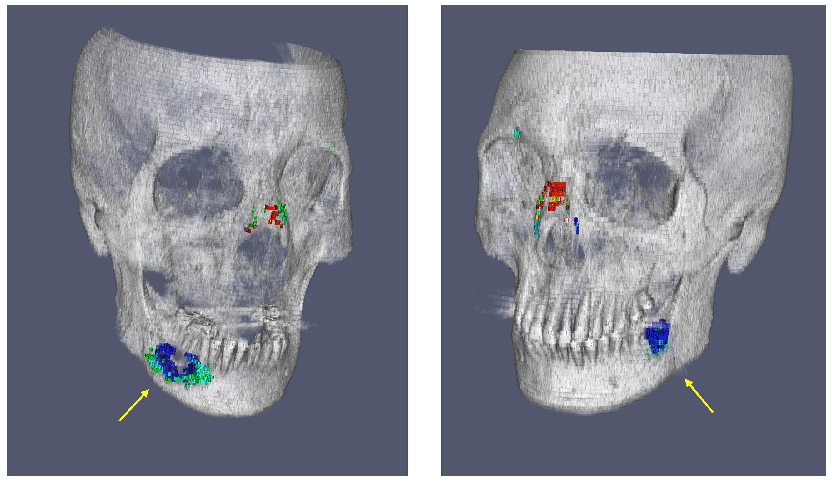
Overall, Figure 7 effectively highlights how the Refined GT group provided a more comprehensive representation of fracture morphology, capturing the true extent of fractures more accurately than the Unrefined GT group. Figure 8 analyzes the differences in key shape features between the two groups. The web-based tool for evaluating deep learning model performance allowed for a comprehensive analysis of segmentation outcomes. Specifically, by approaching fractures through segmentation, the volume of the space between fractured bones could be quantified, enabling a more objective assessment of fracture severity. The platform provides detailed visualizations of the Unrefined GT, Refined GT, and Predict Mask volumes, allowing users to quantify and compare these values. By sorting the volume ratios in ascending or descending order across all test cases, the tool aids in identifying trends in segmentation performance. This includes detecting over- or under-segmentation tendencies between different ground truths. For instance, it was observed that non-fracture-related empty spaces in the mandible, possibly missed in the unrefined GT group, were sometimes identified as fractures, demonstrating the utility of the refined GT in correcting such oversights. This is shown in Figure 9.

Despite these promising results, there are several limitations to our study. First, the segmentation model was trained and validated using data from a single institution, which may limit its generalizability to other clinical settings with different imaging protocols or patient populations. Future studies should include datasets from multiple institutions to enhance the robustness of the model across diverse patient demographics and imaging conditions. Additionally, the current model focuses solely on the segmentation of fracture spaces without differentiating between types of fractures, such as acute versus past fractures. Addressing this limitation will be a key focus of future research, as distinguishing between different types of fractures is crucial for developing more tailored treatment strategies.

Initially, the bounding box regions labeled by medical doctors included deformations caused by old fractures, which were also marked as fractures. Therefore, future research should aim to differentiate clearly between acute fractures, where the fracture line is evident, and deformations which are likely due to old fractures by providing distinct labels for each type.

In conclusion, this study presents a significant advancement in the segmentation of facial bone fractures, providing a foundation for improved diagnostic precision and treatment planning. By refining ground truth datasets and leveraging machine learning techniques, we demonstrated that automated segmentation can achieve a high level of accuracy. Future research will aim to address the current limitations and expand the model’s capabilities, ultimately contributing to better patient care and outcomes in the management of facial bone fractures.

This study has several limitations. First, the segmentation model was developed and validated using data from a single institution, which may limit its generalizability to different clinical settings with varying imaging protocols. Multi-institutional validation is required to enhance the model’s robustness. Second, the proposed approach does not distinguish between acute and chronic fractures, which could provide further insights for personalized treatment planning. Additionally, the stepwise annotation process, while improving segmentation accuracy, remains resource-intensive and may pose scalability challenges. Furthermore, variability in CT image quality and scanner settings could influence segmentation performance, requiring further validation across diverse imaging environments. Lastly, both the unrefined and refined models may exhibit ambiguity in cases where visual assessment alone is subject to interpretation, necessitating careful clinical validation. Addressing these limitations will be crucial for broader clinical adoption and improved performance.

5. Conclusions

In this study, we introduced a novel segmentation model for the spaces between fractured facial bones using CT images, addressing a critical gap in the accurate diagnosis of and treatment planning for facial bone fractures. The proposed segmentation approach leveraged both unrefined and refined ground truth datasets, with significant improvements in segmentation performance, as evidenced by an increase in the Dice similarity coefficient from 0.33 to 0.67. The automated segmentation model demonstrated the ability to accurately delineate fracture regions, enabling the precise analysis of a fracture’s severity and volume. This advancement is of particular importance for clinical practice, where detailed and quantifiable fracture information can support personalized treatment plans and improve outcomes. Our radiomics analysis further validated the consistency between the unrefined and refined ground truth groups, highlighting the enhanced reliability and accuracy achieved through refinement. The developed web-based tool also provides a valuable platform for clinical evaluation, allowing for a detailed examination and comparison of segmentation results in both 2D and 3D contexts.

The main contributions of this study can be summarized as follows. First, we developed a refined segmentation approach by implementing a stepwise annotation process, combining expert-driven initial labeling with automated refinement using the nnU-Net framework. This process significantly improved the segmentation accuracy and reliability. Second, our study introduced a quantitative analysis of inter-fracture spaces, providing objective assessments which are crucial for clinical decision making. Third, radiomics-based validation was conducted to confirm the improved consistency and reduced variability of the refined ground truth. Additionally, we developed a web-based visualization tool to facilitate easy comparison of segmentation results, improving accessibility and usability for clinicians. These contributions collectively demonstrate the potential for integrating automated segmentation into clinical workflows to enhance diagnostic precision and treatment planning.

Overall, our work presents a promising tool for enhancing diagnostic precision and treatment planning for facial bone fractures. Future work will focus on extending the model to differentiate between acute and past fractures and further optimizing the segmentation process to improve efficiency and accuracy.

References

- Figueredo, A.J.; Wolf, P.S.A. Assortative pairing and life history strategy—A cross-cultural study. Hum. Nat. 2009, 20, 317–330. [Google Scholar] [CrossRef]
- Lee, K.H. Interpersonal violence and facial fractures. J. Oral Maxillofac. Surg. 2009, 67, 1878–1883. [Google Scholar] [CrossRef] [PubMed]
- Bakardjiev, A.; Pechalova, P. Maxillofacial fractures in southern bulgaria–a retrospective study of 1706 cases. J.-Cranio-Maxillofac. Surg. 2007, 35, 147–150. [Google Scholar] [CrossRef] [PubMed]
- White, S.C.; Pharoah, M.J. Oral Radiology: Principles and Interpretation; Elsevier Health Sciences: Amsterdam, The Netherland, 2013. [Google Scholar]
- Yu, B.-H.; Han, S.M.; Sun, T.; Guo, Z.; Cao, L.; Wu, H.Z.; Shi, Y.H.; Wen, J.X.; Wu, W.J.; Gao, B.L. Dynamic changes of facial skeletal fractures with time. Sci. Rep. 2020, 10, 4001. [Google Scholar] [CrossRef]
- Gómez Roselló, E.; Quiles Granado, A.M.; Artajona Garcia, M.; Juanpere Martí, S.; Laguillo Sala, G.; Beltrán Mármol, B.; Pedraza Gutiérrez, S. Facial fractures: Classification and highlights for a useful report. Insights Imaging 2020, 11, 49. [Google Scholar] [CrossRef]
- Moon, G.; Kim, S.; Kim, W.; Kim, Y.; Jeong, Y.; Choi, H.S. Computer aided facial bone fracture diagnosis (ca-fbfd) system based on object detection model. IEEE Access 2022, 10, 79061–79070. [Google Scholar] [CrossRef]
- Ukai, K.; Rahman, R.; Yagi, N.; Hayashi, K.; Maruo, A.; Muratsu, H.; Kobashi, S. Detecting pelvic fracture on 3d-ct using deep convolutional neural networks with multi-orientated slab images. Sci. Rep. 2021, 11, 11716. [Google Scholar] [CrossRef]
- Kim, J.; Seo, C.; Yoo, J.H.; Choi, S.H.; Ko, K.Y.; Choi, H.J.; Lee, K.H.; Choi, H.; Shin, D.; Kim, H.; et al. Objective analysis of facial bone fracture ct images using curvature measurement in a surface mesh model. Sci. Rep. 2023, 13, 1932. [Google Scholar] [CrossRef]
- Nam, Y.; Choi, Y.; Kang, J.; Seo, M.; Heo, S.J.; Lee, M.K. Diagnosis of nasal bone fractures on plain radiographs via convolutional neural networks. Sci. Rep. 2022, 12, 21510. [Google Scholar] [CrossRef]
- Jeong, Y.; Jeong, C.; Sung, K.-Y.; Moon, G.; Lim, J. Development of ai-based diagnostic algorithm for nasal bone fracture using deep learning. J. Craniofacial Surg. 2024, 35, 29–32. [Google Scholar] [CrossRef]
- Park, T.; Yoon, M.A.; Cho, Y.C.; Ham, S.J.; Ko, Y.; Kim, S.; Jeong, H.; Lee, J. Automated segmentation of the fractured vertebrae on ct and its applicability in a radiomics model to predict fracture malignancy. Sci. Rep. 2022, 12, 6735. [Google Scholar] [CrossRef]
- Kim, H.; Jeon, Y.D.; Park, K.B.; Cha, H.; Kim, M.S.; You, J.; Lee, S.W.; Shin, S.H.; Chung, Y.G.; Kang, S.B.; et al. Automatic segmentation of inconstant fractured fragments for tibia/fibula from ct images using deep learning. Sci. Rep. 2023, 13, 20431. [Google Scholar] [CrossRef] [PubMed]
- Dreizin, D.; Nam, A.J.; Diaconu, S.C.; Bernstein, M.P.; Bodanapally, U.K.; Munera, F. Multidetector ct of midfacial fractures: Classification systems, principles of reduction, and common complications. Radiographics 2018, 38, 248–274. [Google Scholar] [CrossRef] [PubMed]
- Pham, T.D.; Holmes, S.B.; Coulthard, P. A review on artificial intelligence for the diagnosis of fractures in facial trauma imaging. Front. Artif. Intell. 2024, 6, 1278529. [Google Scholar] [CrossRef]
- Boykov, Y.Y.; Jolly, M.-P. Interactive graph cuts for optimal boundary & region segmentation of objects in nd images. In Proceedings of the Eighth IEEE International Conference on Computer Vision (ICCV 2001), Vancouver, BC, Canada, 7–14 July 2001; Volume 1, pp. 105–112. [Google Scholar] [CrossRef]
- Rother, C.; Kolmogorov, V.; Blake, A. “grabcut” interactive foreground extraction using iterated graph cuts. ACM Trans. Graph. (TOG) 2004, 23, 309–314. [Google Scholar] [CrossRef]
- Müller, D.; Soto-Rey, I.; Kramer, F. Robust chest ct image segmentation of covid-19 lung infection based on limited data. Inform. Med. Unlocked 2021, 25, 100681. [Google Scholar] [CrossRef]
- Yoon, S.H.; Kim, M. Anterior pulmonary ventilation abnormalities in COVID-19. Radiology 2020, 297, E276–E277. [Google Scholar] [CrossRef]
- Inui, S.; Yoon, S.H.; Doganay, O.; Gleeson, F.V.; Kim, M. Impaired pulmonary ventilation beyond pneumonia in COVID-19: A preliminary observation. PLoS ONE 2022, 17, e0263158. [Google Scholar] [CrossRef]
- Park, S.J.; Lee, D.H. Method and Apparatus for Segmenting Medical Images. U.S. Patent No. 10,402,975, 3 September 2019. [Google Scholar]
- Taha, A.A.; Hanbury, A. Metrics for evaluating 3d medical image segmentation: Analysis, selection, and tool. BMC Med. Imaging 2015, 15, 29. [Google Scholar] [CrossRef]
- Maier-Hein, L.; Eisenmann, M.; Reinke, A.; Onogur, S.; Stankovic, M.; Scholz, P.; Arbel, T.; Bogunovic, H.; Bradley, A.P.; Carass, A.; et al. Why rankings of biomedical image analysis competitions should be interpreted with care. Nat. Commun. 2018, 9, 5217. [Google Scholar] [CrossRef]
- Reinke, A.; Tizabi, M.D.; Sudre, C.H.; Eisenmann, M.; Rädsch, T.; Baumgartner, M.; Acion, L.; Antonelli, M.; Arbel, T.; Bakas, S.; et al. Common limitations of image processing metrics: A picture story. arXiv 2021, arXiv:2104.05642. [Google Scholar] [CrossRef]
- Zou, K.H.; Warfield, S.K.; Bharatha, A.; Tempany, C.M.; Kaus, M.R.; Haker, S.J.; Wells, I.I.I.W.M.; Jolesz, F.A.; Kikinis, R. Statistical validation of image segmentation quality based on a spatial overlap index1: Scientific reports. Acad. Radiol. 2004, 11, 178–189. [Google Scholar] [CrossRef] [PubMed]
- Yushkevich, P.A.; Piven, J.; Hazlett, H.C.; Smith, R.G.; Ho, S.; Gee, J.C.; Gerig, G. User-guided 3d active contour segmentation of anatomical structures: Significantly improved efficiency and reliability. Neuroimage 2006, 31, 1116–1128. [Google Scholar] [CrossRef] [PubMed]
- Furtado, P. Testing segmentation popular loss and variations in three multiclass medical imaging problems. J. Imaging 2021, 7, 16. [Google Scholar] [CrossRef]
- Isensee, F.; Jaeger, P.F.; Kohl, S.A.; Petersen, J.; Maier-Hein, K.H. nnu-net: A self-configuring method for deep learning-based biomedical image segmentation. Nat. Methods 2021, 18, 203–211. [Google Scholar] [CrossRef]
- Kitware, I. Vtk.js—The Visualization Toolkit for Javascript. 2023. Available online: https://kitware.github.io/vtk-js/index.html (accessed on 24 January 2024).
- Dho, Y.-S.; Lee, D.; Ha, T.; Ji, S.Y.; Kim, K.M.; Kang, H.; Kim, M.S.; Kim, J.W.; Cho, W.S.; Kim, Y.H.; et al. Clinical application of patient-specific 3d printing brain tumor model production system for neurosurgery. Sci. Rep. 2021, 11, 7005. [Google Scholar] [CrossRef]
- Abdi, H. Bonferroni and šidák corrections for multiple comparisons. Encycl. Meas. Stat. 2007, 3, 2007. [Google Scholar]
Figure 1.
Process of creating initial ground truth segmentation. The left image (“1st Approach”) shows the fracture areas outlined by clinical specialists using red bounding boxes in a dual plane. The right image (“2nd Approach”) illustrates the initial ground truth segmentation derived from the “1st Approach”, with the fracture areas represented in red.
Figure 2.
Initial ground truth segmentation performed using ITK-SNAP.
Figure 3.
Refinement workflow. Initially, medical doctors (MDs) provided bounding boxes for the fracture regions. These bounding boxes were then used by labelers to create initial segmentation masks (Unrefined GT) for 1766 cases. The nnUnet framework was applied to the entire dataset to generate refined segmentation masks (Refined GT) for all 1766 cases, with additional predicted segmentation masks (Predict GT) created for a subset of 282 cases (20%) to assess performance.
Figure 4.
Box plot illustrating the normalized radiomics feature values extracted from the refined and unrefined ground truth datasets. Radiomics feature extraction was performed to facilitate a comparative analysis between the refined and unrefined segmentations, highlighting the variability in feature values across different segmentation approaches. Normalization was applied to allow for consistent comparison across features with varying ranges. Of the 107 total features, only the 70 features with Bonferroni-corrected p values greater than 0.01 are displayed.