
Spectrum Attention Mechanism-Based Acoustic Vector DOA Estimation Method in the Presence of Colored Noise

Abstract
1. Introduction
2. Problem Description
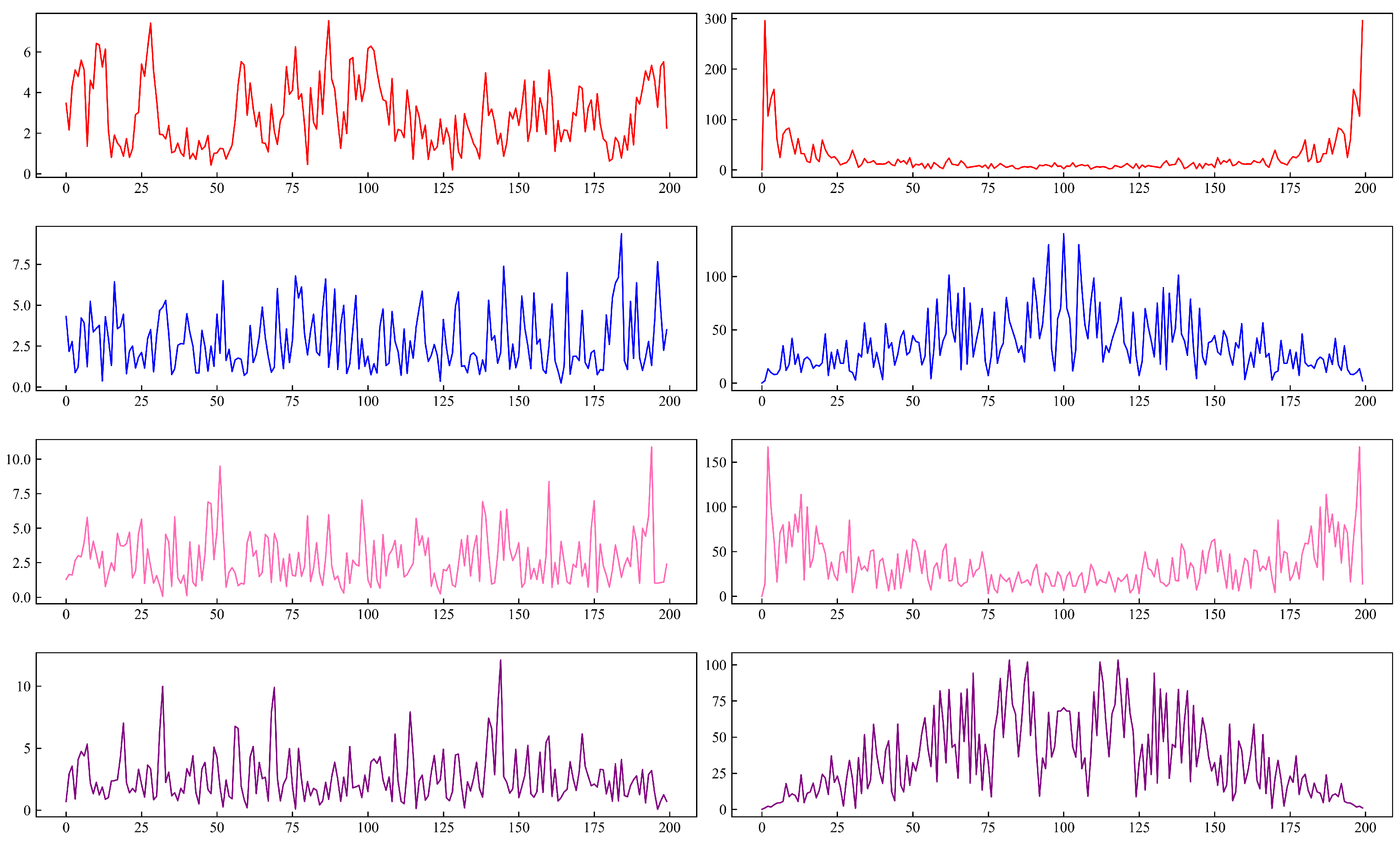
2.1. Colored Noise
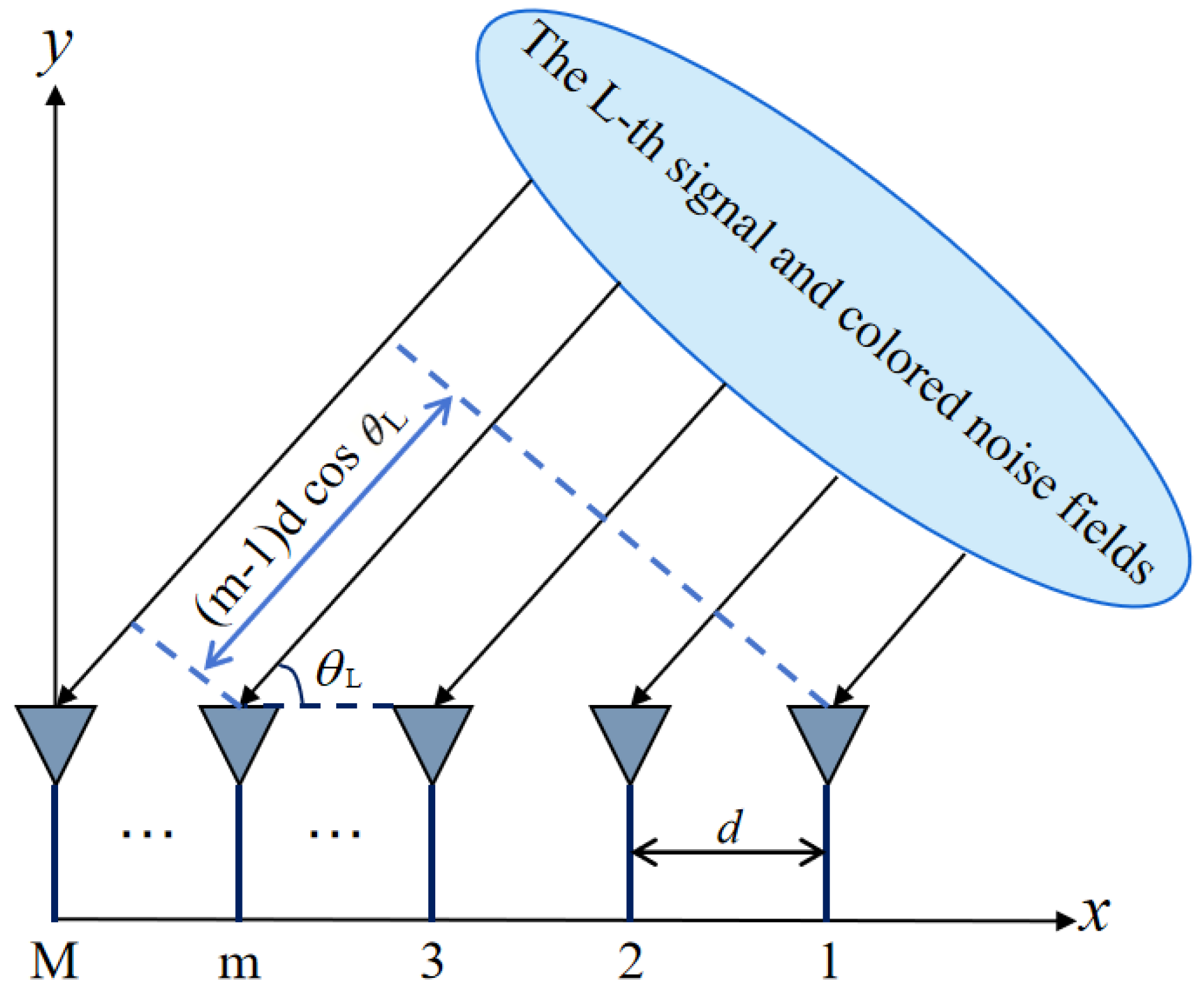
2.2. Array Signal Model
3. Methodology
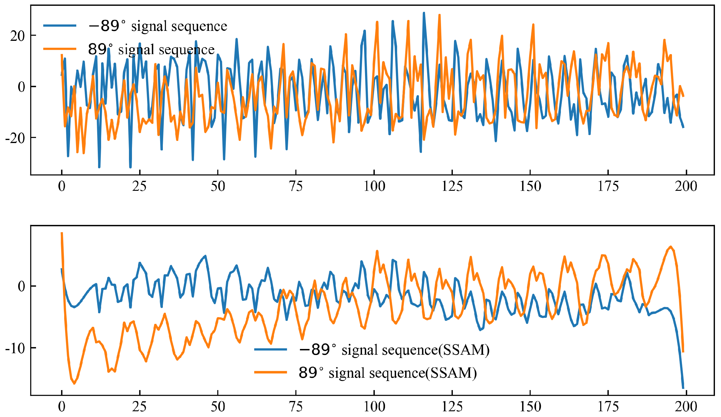
3.1. SAM
| Algorithm 1 Spectrum Attention Mechanism (SAM) |
| Input: Captured signal sequence Output:
|
| Algorithm 2 Segmented SAM (SSAM) |
| Input: , number of segments K Output: generated features
|
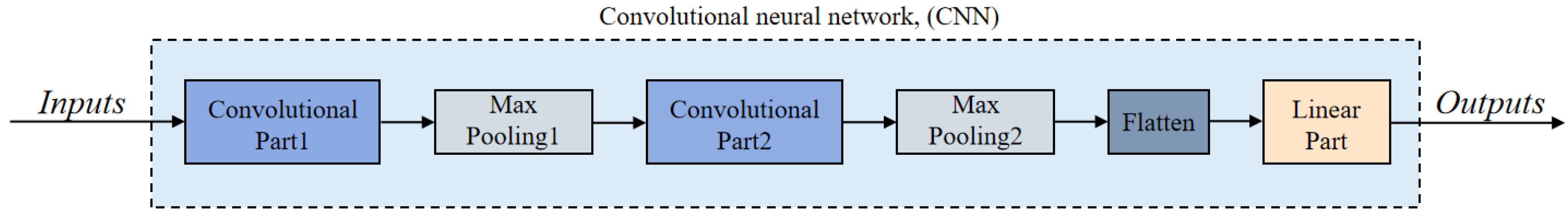
3.2. CNN
- (1)
- Convolutional layer
- (2)
- Pooling layer
3.3. LSTM
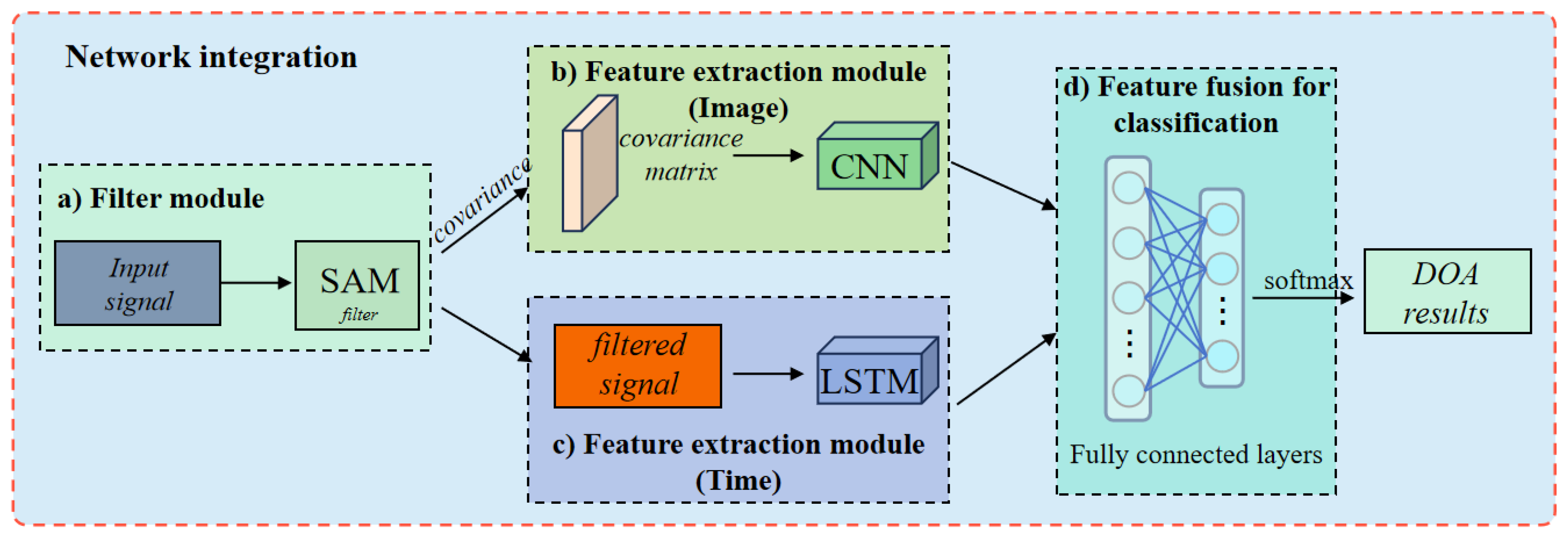
3.4. Network Integration
4. Experimental Results
4.1. Training Data
4.2. Filter Results
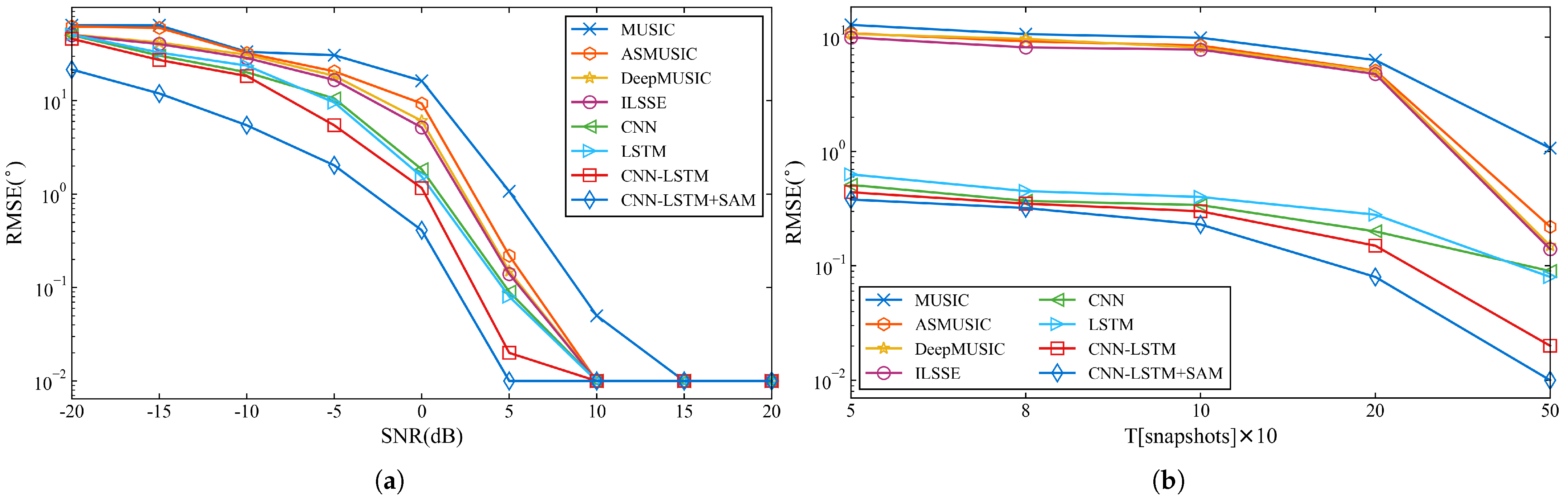
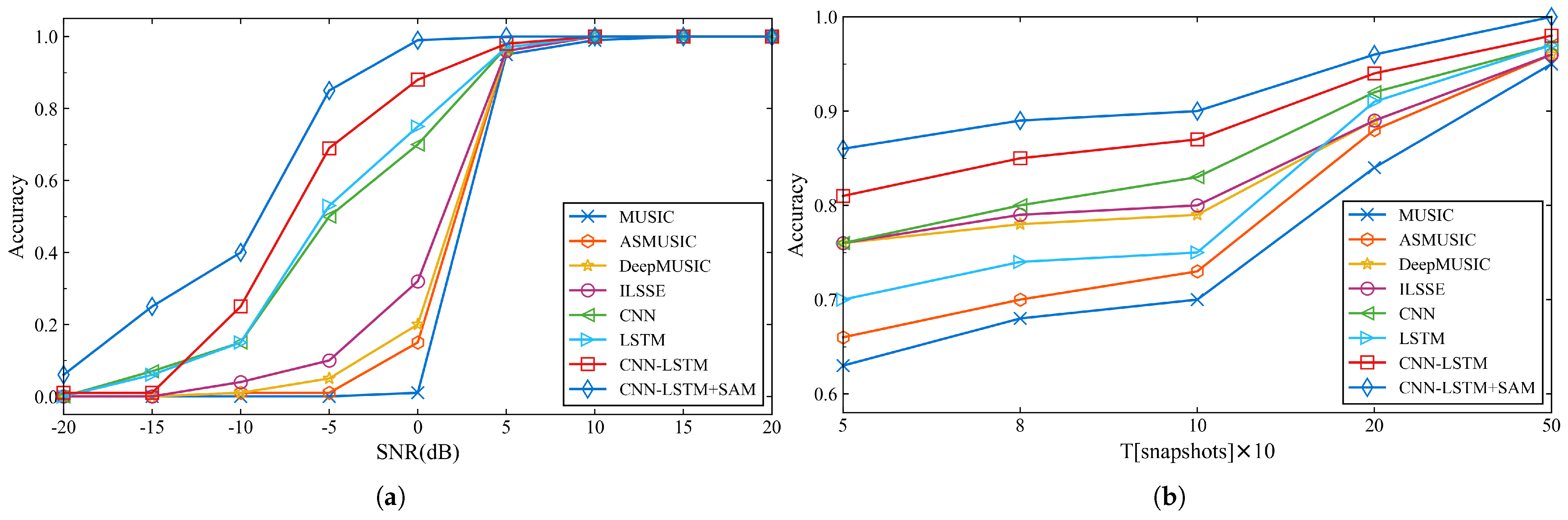
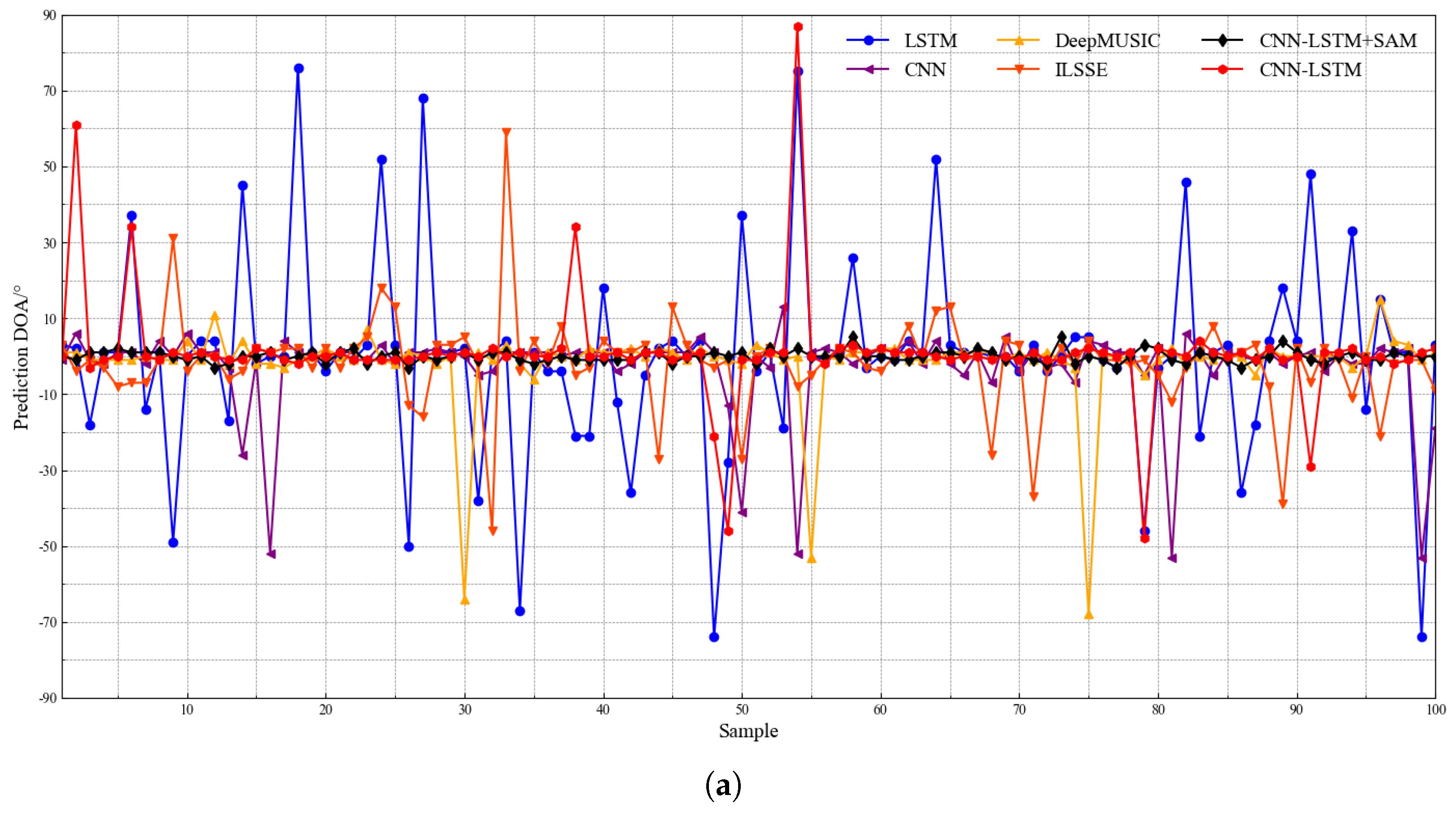
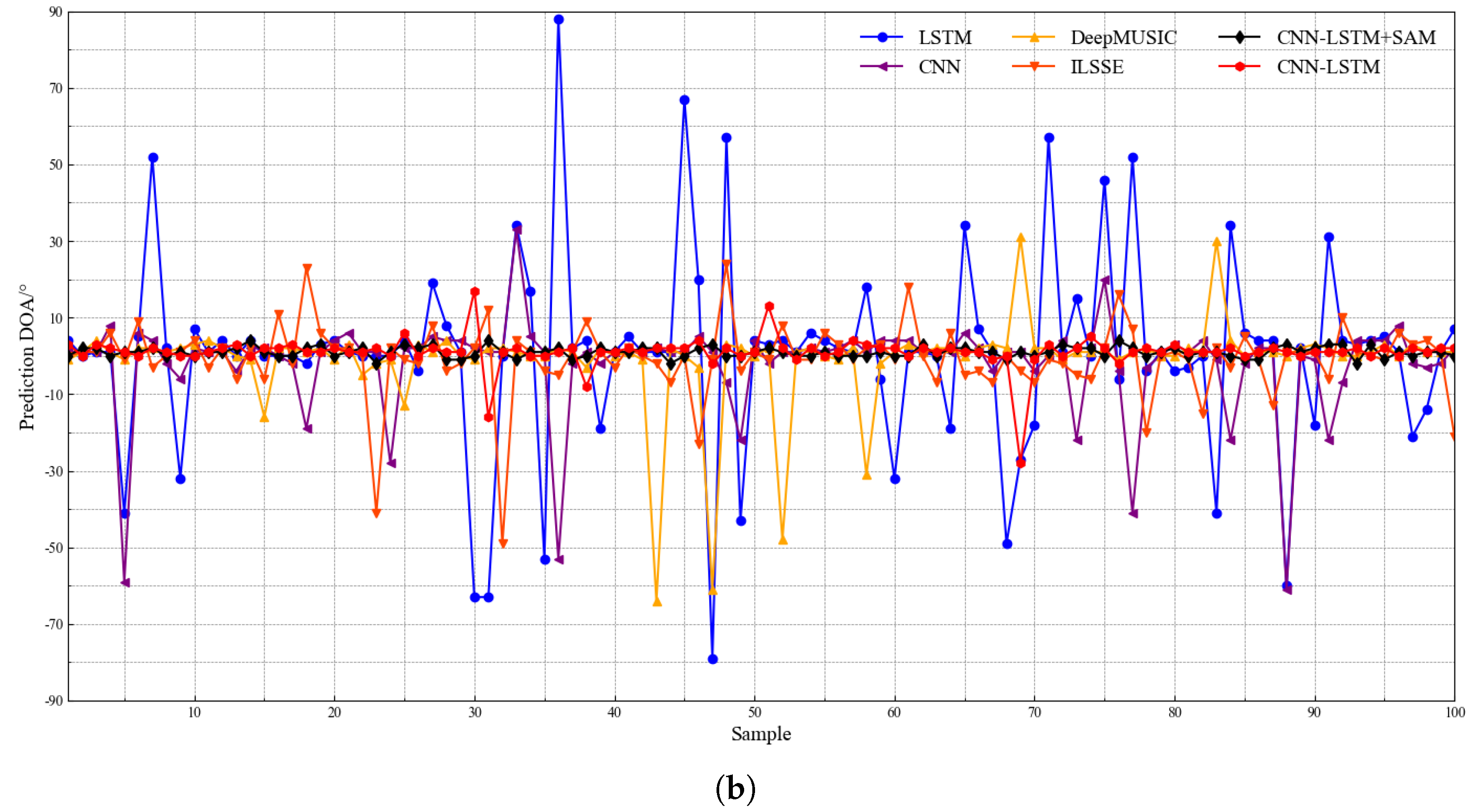
4.3. Performance of DOA Estimation Model
5. Conclusions
Author Contributions
Funding
Institutional Review Board Statement
Informed Consent Statement
Data Availability Statement
Acknowledgments
Conflicts of Interest
References
- Liu, Y.; Tan, Z.W.; Khong, A.W.H.; Liu, H. Joint Source Localization and Association Through Overcomplete Representation Under Multipath Propagation Environment. In Proceedings of the ICASSP 2022—2022 IEEE International Conference on Acoustics, Speech and Signal Processing (ICASSP), Singapore, 23–27 May 2022; pp. 5123–5127. [Google Scholar]
- Shi, W.; Huang, J.; Hou, Y. Fast DOA estimation algorithm for MIMO sonar based on ant colony optimization. J. Syst. Eng. Electron. 2012, 23, 173–178. [Google Scholar] [CrossRef]
- Chen, Y.; Yan, L.; Han, C.; Tao, M. Millidegree-Level Direction-of-Arrival Estimation and Tracking for Terahertz Ultra-Massive MIMO Systems. IEEE Trans. Wirel. Commun. 2022, 21, 869–883. [Google Scholar] [CrossRef]
- Chen, F.; Yang, D.; Mo, S. A DOA Estimation Algorithm Based on Eigenvalues Ranking Problem. IEEE Trans. Instrum. Meas. 2023, 72, 9501315. [Google Scholar] [CrossRef]
- Zou, N.; Nehorai, A. Circular acoustic vector-sensor array for mode beamforming. IEEE Trans. Signal Process. 2009, 57, 3041–3052. [Google Scholar] [CrossRef]
- Shi, S.; Li, Y.; Yang, D.; Liu, A.; Shi, J. Sparse representation based direction-of-arrival estimation using circular acoustic vector sensor arrays. Digit. Signal Process. 2020, 99, 102675. [Google Scholar] [CrossRef]
- Cray, B.; Nuttall, A. Directivity factors for linear arrays of velocity sensors. J. Acoust. Soc. Am. 2001, 110, 324–331. [Google Scholar] [CrossRef]
- Mathews, C.P.; Zoltowski, M.D. Eigenstructure Techniques for 2-D Angle Estimation with Uniform Circular Arrays. IEEE Trans. Signal Process. 1994, 42, 2395–2407. [Google Scholar] [CrossRef]
- Nehorai, A.; Paldi, E. Acoustic Vector-Sensor Array Processing. IEEE Trans. Signal Process. 1994, 42, 2481–2491. [Google Scholar] [CrossRef]
- Hawkes, M. Acoustic vector-sensor beamforming and capon direction estimation. IEEE Trans. Signal Process. 1998, 46, 2291–2304. [Google Scholar] [CrossRef] [PubMed]
- Schmidt, R.O. Multiple emitter location and signal parameter estimation. IEEE Trans. Antennas Propag. 1986, AP-34, 276–280. [Google Scholar] [CrossRef]
- Xu, X.; Xue, Y.; Fang, Q.; Qiao, Z.; Liu, S.; Wang, X.; Tang, R. Hybrid nanoparticles based on ortho ester-modified pluronic L61 and chitosan for efficient doxorubicin delivery. Int. J. Biol. Macromol. 2021, 183, 1596–1606. [Google Scholar] [CrossRef] [PubMed]
- Liao, B.; Huang, L.; Guo, C.; So, H.C. New Approaches to Direction-of-Arrival Estimation with Sensor Arrays in Unknown Nonuniform Noise. IEEE Sens. J. 2016, 16, 8982–8989. [Google Scholar] [CrossRef]
- Stoica, P.; Nehorai, A. Music, Maximum Likelihood, And Cramer-Rao Bound. IEEE Trans. Acoust. Speech Signal Process. 1989, 37, 720–741. [Google Scholar] [CrossRef]
- Chen, C.E.; Lorenzelli, F.; Hudson, R.E.; Yao, K. Stochastic maximum-likelihood DOA estimation in the presence of unknown nonuniform noise. IEEE Trans. Signal Process. 2008, 56, 3038–3044. [Google Scholar] [CrossRef]
- Madurasinghe, D. A new DOA estimator in nonuniform noise. IEEE Signal Process. Lett. 2005, 12, 337–339. [Google Scholar] [CrossRef]
- Wu, Y.; Hou, C.; Liao, G.; Guo, Q. Direction-of-arrival estimation in the presence of unknown nonuniform noise fields. IEEE J. Ocean. Eng. 2006, 31, 504–510. [Google Scholar] [CrossRef]
- Liao, B.; Chan, S.C.; Huang, L.; Guo, C. Iterative Methods for Subspace and DOA Estimation in Nonuniform Noise. IEEE Trans. Signal Process. 2016, 64, 3008–3020. [Google Scholar] [CrossRef]
- He, Z.Q.; Shi, Z.P.; Huang, L. Covariance sparsity-aware DOA estimation for nonuniform noise. Digit. Signal Process. 2014, 28, 75–81. [Google Scholar] [CrossRef]
- Liu, A.; Yang, D.; Shi, S.; Zhu, Z.; Li, Y. Augmented subspace MUSIC method for DOA estimation using acoustic vector sensor array. IET Radar Sonar Navig. 2019, 13, 969–975. [Google Scholar] [CrossRef]
- Wang, W.; Zhang, Q.; Shi, W.; Tan, W.; Mao, L. Off-Grid DOA Estimation Based on Alternating Iterative Weighted Least Squares for Acoustic Vector Hydrophone Array. Circuits Syst. Signal Process. 2020, 39, 4650–4680. [Google Scholar] [CrossRef]
- Liu, Y.; Chen, H.; Wang, B. DOA estimation based on CNN for underwater acoustic array. Appl. Acoust. 2021, 172, 107594. [Google Scholar] [CrossRef]
- Papageorgiou, G.K.; Sellathurai, M.; Eldar, Y.C. Deep Networks for Direction-of-Arrival Estimation in Low SNR. IEEE Trans. Signal Process. 2021, 69, 3714–3729. [Google Scholar] [CrossRef]
- Elbir, A.M. DeepMUSIC: Multiple Signal Classification via Deep Learning. IEEE Sens. Lett. 2020, 4, 7001004. [Google Scholar] [CrossRef]
- Liu, K.; Wang, X.; Yu, J.; Ma, J. Attention based DOA estimation in the presence of unknown nonuniform noise. Appl. Acoust. 2023, 211, 109506. [Google Scholar] [CrossRef]
- Zhou, S.; Pan, Y. Spectrum Attention Mechanism for Time Series Classification. In Proceedings of the 2021 IEEE 10th Data Driven Control and Learning Systems Conference (DDCLS), Suzhou, China, 14–16 May 2021; pp. 339–343. [Google Scholar] [CrossRef]


| Methods | −20 dB | −15 dB | −10 dB | −5 dB | 0 dB | 5 dB | 10 dB | 15 dB | 20 dB |
|---|---|---|---|---|---|---|---|---|---|
| MUSIC | 64.03 | 63.89 | 33.29 | 30.63 | 16.31 | 1.07 | 0.05 | 0.01 | 0.01 |
| ASMUSIC | 62.11 | 60.08 | 32.35 | 20.55 | 9.33 | 0.22 | 0.01 | 0.01 | 0.01 |
| DeepMUSIC | 50.91 | 41.92 | 30.88 | 18.43 | 6.08 | 0.15 | 0.01 | 0.01 | 0.01 |
| ILSSE | 50.12 | 40.32 | 28.59 | 16.65 | 5.16 | 0.14 | 0.01 | 0.01 | 0.01 |
| CNN | 50.09 | 30.31 | 20.11 | 10.56 | 1.84 | 0.09 | 0.01 | 0.01 | 0.01 |
| LSTM | 50.80 | 32.71 | 23.68 | 9.55 | 1.54 | 0.08 | 0.01 | 0.01 | 0.01 |
| CNN-LSTM | 45.92 | 27.22 | 18.32 | 5.44 | 1.16 | 0.02 | 0.01 | 0.01 | 0.01 |
| CNN-LSTM+SAM | 21.51 | 11.93 | 5.45 | 2.03 | 0.41 | 0.01 | 0.01 | 0.01 | 0.01 |
| Methods | 50 Snapshots | 80 Snapshots | 100 Snapshots | 200 Snapshots | 500 Snapshots |
|---|---|---|---|---|---|
| MUSIC | 12.78 | 10.61 | 9.87 | 6.29 | 1.07 |
| ASMUSIC | 10.79 | 9.18 | 8.44 | 5.10 | 0.22 |
| DeepMUSIC | 10.65 | 9.63 | 8.08 | 5.02 | 0.15 |
| ILSSE | 9.92 | 8.12 | 7.77 | 4.75 | 0.14 |
| CNN | 0.51 | 0.37 | 0.34 | 0.20 | 0.09 |
| LSTM | 0.63 | 0.45 | 0.40 | 0.28 | 0.08 |
| CNN-LSTM | 0.44 | 0.35 | 0.30 | 0.15 | 0.02 |
| CNN-LSTM+SAM | 0.38 | 0.32 | 0.23 | 0.08 | 0.01 |
| Methods | −20 dB | −15 dB | −10 dB | −5 dB | 0 dB | 5 dB | 10 dB | 15 dB | 20 dB |
|---|---|---|---|---|---|---|---|---|---|
| MUSIC | 0% | 0% | 0% | 0% | 1% | 95% | 99% | 100% | 100% |
| ASMUSIC | 0% | 0% | 1% | 1% | 15% | 96% | 100% | 100% | 100% |
| DeepMUSIC | 0% | 0% | 1% | 5% | 20% | 96% | 100% | 100% | 100% |
| ILSSE | 0% | 0% | 4% | 10% | 32% | 96% | 100% | 100% | 100% |
| CNN | 0% | 7% | 15% | 50% | 70% | 97% | 100% | 100% | 100% |
| LSTM | 0% | 6% | 15% | 53% | 75% | 97% | 100% | 100% | 100% |
| CNN-LSTM | 1% | 14% | 25% | 69% | 88% | 98% | 100% | 100% | 100% |
| CNN-LSTM+SAM | 6% | 25% | 40% | 85% | 99% | 100% | 100% | 100% | 100% |
| Methods | 50 Snapshots | 80 Snapshots | 100 Snapshots | 200 Snapshots | 500 Snapshots |
|---|---|---|---|---|---|
| MUSIC | 63% | 68% | 70% | 84% | 95% |
| ASMUSIC | 66% | 70% | 73% | 88% | 96% |
| DeepMUSIC | 76% | 78% | 79% | 89% | 96% |
| ILSSE | 76% | 79% | 80% | 89% | 96% |
| CNN | 76% | 80% | 83% | 92% | 97% |
| LSTM | 70% | 74% | 75% | 91% | 97% |
| CNN-LSTM | 81% | 85% | 87% | 94% | 98% |
| CNN-LSTM+SAM | 86% | 89% | 90% | 96% | 100% |
Disclaimer/Publisher’s Note: The statements, opinions and data contained in all publications are solely those of the individual author(s) and contributor(s) and not of MDPI and/or the editor(s). MDPI and/or the editor(s) disclaim responsibility for any injury to people or property resulting from any ideas, methods, instructions or products referred to in the content. |
© 2025 by the authors. Licensee MDPI, Basel, Switzerland. This article is an open access article distributed under the terms and conditions of the Creative Commons Attribution (CC BY) license (https://creativecommons.org/licenses/by/4.0/).
Share and Cite
Xu, W.; Liu, M.; Yi, S. Spectrum Attention Mechanism-Based Acoustic Vector DOA Estimation Method in the Presence of Colored Noise. Appl. Sci. 2025, 15, 1473. https://doi.org/10.3390/app15031473
Xu W, Liu M, Yi S. Spectrum Attention Mechanism-Based Acoustic Vector DOA Estimation Method in the Presence of Colored Noise. Applied Sciences. 2025; 15(3):1473. https://doi.org/10.3390/app15031473
Chicago/Turabian StyleXu, Wenjie, Mindong Liu, and Shichao Yi. 2025. "Spectrum Attention Mechanism-Based Acoustic Vector DOA Estimation Method in the Presence of Colored Noise" Applied Sciences 15, no. 3: 1473. https://doi.org/10.3390/app15031473
APA StyleXu, W., Liu, M., & Yi, S. (2025). Spectrum Attention Mechanism-Based Acoustic Vector DOA Estimation Method in the Presence of Colored Noise. Applied Sciences, 15(3), 1473. https://doi.org/10.3390/app15031473