
Using Hybrid LSTM Neural Networks to Detect Anomalies in the Fiber Tube Manufacturing Process


Abstract
1. Introduction
2. Materials and Methods
2.1. Factory RLM Line Data Acquisition
2.2. Preprocessing of Input Data for Training Set
 ,
,  and
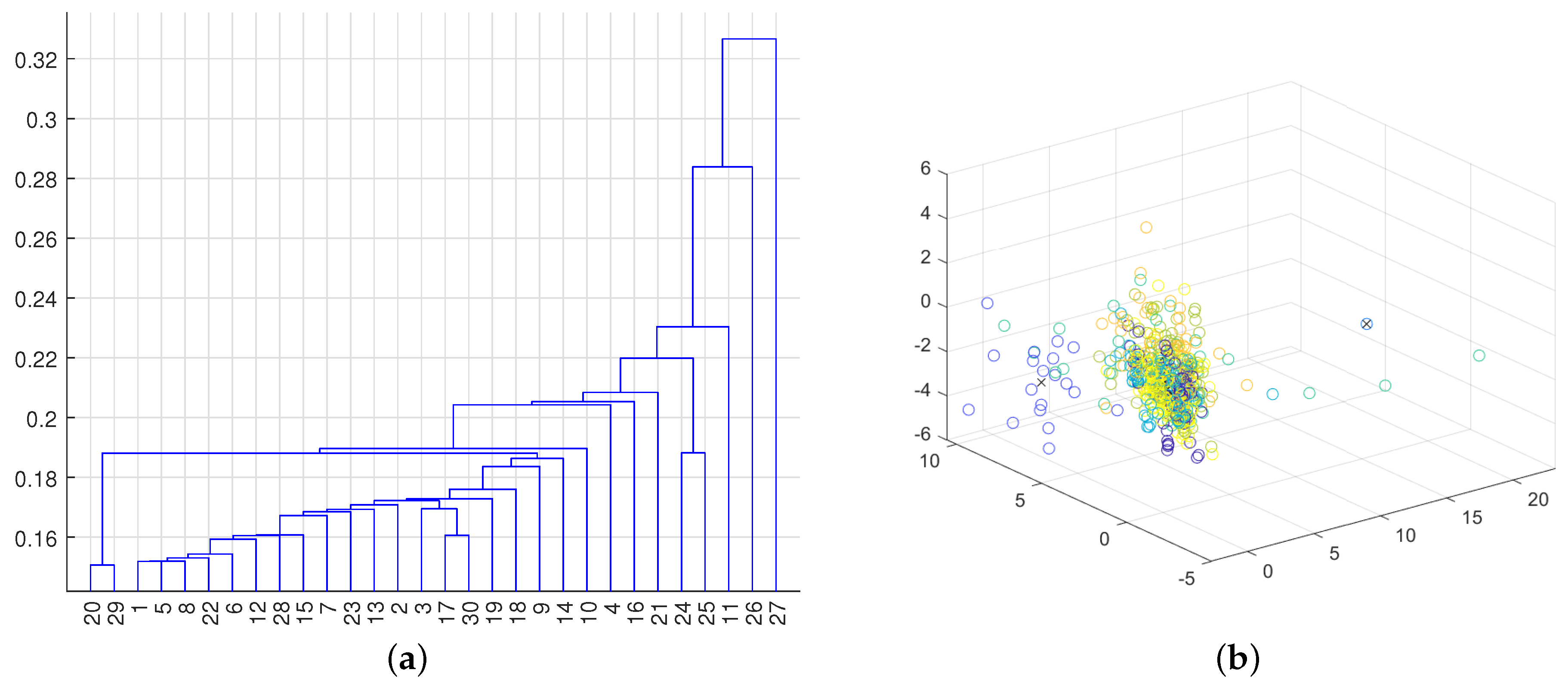
and  stand for: the waveform of the components of the DWT transform, the waveforms of the leading 40 components of the production process, and the membership of the RLM line signal to the different classes extracted in the clustering process. The left column (Figure 2a,c,e,g,i,k) corresponds to the decomposition of the signal recorded during the measurement session from the RLM production line using a 4–octave Haar–based DWT, while the right column (Figure 2b,d,f,h,j,l) corresponds to the decomposition of the same signal using a 2–octave Haar–based DWT. The waveforms (Figure 2a–d) show example sections of RLM line acceleration, in which the time interval is marked with a rectangular area. The symbols and , denote the start of the fiber twisting process and the end of the twisting process of a given tube section, respectively. Graphs (Figure 2e–h) contain waveforms for the ongoing basic production process also for two different randomly selected sessions. The recorded process data from the RLM line , were normalized for each signal channel data independently: represent an attempt to visualize the potential membership of the production process state to a priori selected number of classes.
2.3. Hybrid LSTM Network Model for Anomaly Detection
3. Results and Discussion

- Anomaly 1: Excessive fluctuations in pressure and temperature alter the geometry and texture of the produced item. Significant pressure variations cause diameter changes within the range of 0.2 [mm] to 0.4 [mm], leading to the product being classified as non–compliant. In the cable coating extrusion process, large pressure changes result in discontinuities in the coating material, causing the final product to be divided into short segments, which are often unacceptable to customers.
- Anomaly 2: Excessive deviations in the pressure and temperature of the hydrophobic gel. Pressure changes lead to variations in the external and internal diameters of the semi–finished product. Changes in the external diameter result in weakened strength at the constriction points of the semi–finished product.
- Anomaly 3: Excessive production speed and the associated tension force of the production line and winding device. According to experts, this is a crucial anomaly that causes excess fiber in the tube, negatively affecting the transmission properties and strength of the finished fiber optic cable. Moreover, its frequent occurrence indicates wear and tear of the drive and consumable parts of the line.
- Anomaly 4: Temperature fluctuations in the cooling bath water affect the surface condition of semi–finished and finished products, as well as the dynamics of secondary shrinkage, which negatively impacts semi–finished and finished cables many days after their production.
4. Conclusions
Author Contributions
Funding
Institutional Review Board Statement
Informed Consent Statement
Data Availability Statement
Acknowledgments
Conflicts of Interest
Abbreviations
| DNN | Deep Neural Network |
| DWT | Discrete Wavelet Transform |
| LSTM | Long short-term memory |
| RNN | Recurrent neural network |
| RLR | line for tube extrusion |
| RLV | line for coating extrusion on the cable core |
| RLM | line for twisting cable cores from tubes |
| SVM | Support Vector Machines |
References
- Gordan, M.; Sabbagh-Yazdi, S.R.; Ismail, Z.; Ghaedi, K.; Carroll, P.; McCrum, D.; Samali, B. State-of-the-art review on advancements of data mining in structural health monitoring. Measurement 2022, 193, 110939. [Google Scholar] [CrossRef]
- Kotsiopoulos, T.; Sarigiannidis, P.; Ioannidis, D.; Tzovaras, D. Machine Learning and Deep Learning in smart manufacturing: The Smart Grid paradigm. Comput. Sci. Rev. 2021, 40, 100341. [Google Scholar] [CrossRef]
- Ribeiro, R.; Pilastri, A.; Moura, C.; Morgado, J.; Cortez, P. A data-driven intelligent decision support system that combines predictive and prescriptive analytics for the design of new textile fabrics. Neural Comput. Appl. 2023, 35, 17375–17395. [Google Scholar] [CrossRef]
- Bock, F.E.; Aydin, R.C.; Cyron, C.J.; Huber, N.; Kalidindi, S.R.; Klusemann, B. A review of the application of machine learning and data mining approaches in continuum materials mechanics. Front. Mater. 2019, 6, 452701. [Google Scholar] [CrossRef]
- Soleimani, M.; Naderian, H.; Afshinfar, A.H.; Savari, Z.; Tizhari, M.; Agha Seyed Hosseini, S.R. A Method for Predicting Production Costs Based on Data Fusion from Multiple Sources for Industry 4.0: Trends and Applications of Machine Learning Methods. Comput. Intell. Neurosci. 2023, 2023, 6271241. [Google Scholar] [CrossRef] [PubMed]
- Abdallah, M.; Joung, B.G.; Lee, W.J.; Mousoulis, C.; Raghunathan, N.; Shakouri, A.; Sutherland, J.W.; Bagchi, S. Anomaly Detection and Inter-Sensor Transfer Learning on Smart Manufacturing Datasets. Sensors 2023, 23, 486. [Google Scholar] [CrossRef] [PubMed]
- Abdelli, K.; Cho, J.Y.; Azendorf, F.; Griesser, H.; Tropschug, C.; Pachnicke, S. Machine Learning-based Anomaly Detection in Optical Fiber Monitoring. J. Opt. Commun. Netw. 2022, 14, 365–375. [Google Scholar] [CrossRef]
- Abdula, S.P.; Llagas, M.J.; Fernandez, A.M.; Arboleda, E. Machine Learning Applications for Fault Tracing and Localization in Optical Fiber Communication Networks: A Review. Preprints 2024. [Google Scholar] [CrossRef]
- Glass, S.W.; Fifield, L.S.; Spencer, M.P. Transition to Online Cable Insulation Condition Monitoring. In Proceedings of the 2021 48th Annual Review of Progress in Quantitative Nondestructive Evaluation, QNDE 2021, Virtual, 28–30 July 2021. [Google Scholar]
- Kakavandi, F.; Gomes, C.; de Reus, R.; Badstue, J.; Jensen, J.L.; Larsen, P.G.; Iosifidis, A. Towards Developing a Digital Twin for a Manufacturing Pilot Line: An Industrial Case Study. In Digital Twin Driven Intelligent Systems and Emerging Metaverse; Springer: Singapore, 2023; pp. 39–64. [Google Scholar]
- Kane, A.P.; Kore, A.S.; Khandale, A.N.; Nigade, S.S.; Joshi, P.P. Predictive Maintenance Using Machine Learning; SPD Technology: London, UK, 2022. [Google Scholar]
- Pittino, F.; Puggl, M.; Moldaschl, T.; Hirschl, C. Automatic Anomaly Detection on In-Production Manufacturing Machines Using Statistical Learning Methods. Sensors 2020, 20, 2344. [Google Scholar] [CrossRef]
- Fan, J.; Wang, Z.; Wu, H.; Sun, D.; Wu, J.; Lu, X. An Adversarial Time–Frequency Reconstruction Network for Unsupervised Anomaly Detection. Neural Netw. 2023, 168, 44–56. [Google Scholar] [CrossRef] [PubMed]
- Zhu, W.; Li, W.; Dorsey, E.R.; Luo, J. Unsupervised anomaly detection by densely contrastive learning for time series data. Neural Netw. 2023, 168, 450–458. [Google Scholar] [CrossRef] [PubMed]
- Zhang, X.; Shi, S.; Sun, H.; Chen, D.; Wang, G.; Wu, K. ACVAE: A novel self-adversarial variational auto-encoder combined with contrast learning for time series anomaly detection. Neural Netw. 2024, 171, 383–395. [Google Scholar] [CrossRef] [PubMed]
- Yao, Y.; Ma, J.; Feng, S.; Ye, Y. SVD-AE: An asymmetric autoencoder with SVD regularization for multivariate time series anomaly detection. Neural Netw. 2024, 170, 535–547. [Google Scholar] [CrossRef] [PubMed]
- Li, Q.; Wang, Y.; Dong, J.; Zhang, C.; Peng, K. Multi-node knowledge graph assisted distributed fault detection for large-scale industrial processes based on graph attention network and bidirectional LSTMs. Neural Netw. 2024, 173, 106210. [Google Scholar] [CrossRef] [PubMed]
- Fan, J.; Ge, Y.; Zhang, X.; Wang, Z.; Wu, H.; Wu, J. Learning the feature distribution similarities for online time series anomaly detection. Neural Netw. 2024, 180, 106638. [Google Scholar] [CrossRef] [PubMed]
- Lyu, S.; Mo, D.; Wong, W.K. REB: Reducing biases in representation for industrial anomaly detection. Knowl.-Based Syst. 2024, 290, 111563. [Google Scholar] [CrossRef]
- Kang, B.; Zhong, Y.; Sun, Z.; Deng, L.; Wang, M.; Zhang, J. MSTAD: A masked subspace-like transformer for multi-class anomaly detection. Knowl.-Based Syst. 2024, 283, 111186. [Google Scholar] [CrossRef]
- Iqbal Basheer, M.Y.; Mohd Ali, A.; Abdul Hamid, N.H.; Mohd Ariffin, M.A.; Osman, R.; Nordin, S.; Gu, X. Autonomous anomaly detection for streaming data. Knowl.-Based Syst. 2024, 284, 111235. [Google Scholar] [CrossRef]
- Hong, J.; Kang, S. Score distillation for anomaly detection. Knowl.-Based Syst. 2024, 295, 111842. [Google Scholar] [CrossRef]
- Wang, X.; Li, W.; He, X. MTDiff: Visual anomaly detection with multi-scale diffusion models. Knowl.-Based Syst. 2024, 302, 112364. [Google Scholar] [CrossRef]
- Guo, W.; Jiang, P. Weakly Supervised anomaly detection with privacy preservation under a Bi-Level Federated learning framework. Expert Syst. Appl. 2024, 254, 124450. [Google Scholar] [CrossRef]
- An, S.; Kim, J.; Kim, S.; Chikontwe, P.; Jung, J.; Jeon, H.; Park, S.H. Few-shot anomaly detection using positive unlabeled learning with cycle consistency and co-occurrence features. Expert Syst. Appl. 2024, 256, 124890. [Google Scholar] [CrossRef]
- Shen, L.; Wei, Y.; Wang, Y.; Li, H. AFMF: Time series anomaly detection framework with modified forecasting. Knowl.-Based Syst. 2024, 296, 111912. [Google Scholar] [CrossRef]
- Bai, Y.; Zhang, J.; Chen, Z.; Dong, Y.; Cao, Y.; Tian, G. Dual-path Frequency Discriminators for few-shot anomaly detection. Knowl.-Based Syst. 2024, 302, 112397. [Google Scholar] [CrossRef]
- Liu, Y.; Ju, B.; Yang, D.; Peng, L.; Li, D.; Sun, P.; Li, C.; Yang, H.; Liu, J.; Song, L. Memory-enhanced spatial-temporal encoding framework for industrial anomaly detection system. Expert Syst. Appl. 2024, 250, 123718. [Google Scholar] [CrossRef]
- Di, Y.; Wang, F.; Zhao, Z.; Zhai, Z.; Chen, X. An interpretable graph neural network for real-world satellite power system anomaly detection based on graph filtering. Expert Syst. Appl. 2024, 254, 124348. [Google Scholar] [CrossRef]
- Chen, A.; Wu, J.; Zhang, H. FIAD: Graph anomaly detection framework based feature injection. Expert Syst. Appl. 2025, 259, 125216. [Google Scholar] [CrossRef]
- Lei, T.; Ou, M.; Gong, C.; Li, J.; Yang, K. An unsupervised deep global–local views model for anomaly detection in attributed networks. Knowl.-Based Syst. 2024, 300, 112185. [Google Scholar] [CrossRef]
- Mejri, N.; Lopez-Fuentes, L.; Roy, K.; Chernakov, P.; Ghorbel, E.; Aouada, D. Unsupervised anomaly detection in time-series: An extensive evaluation and analysis of state-of-the-art methods. Expert Syst. Appl. 2024, 256, 124922. [Google Scholar] [CrossRef]
- Chi, J.; Mao, Z. Deep domain-adversarial anomaly detection with robust one-class transfer learning. Knowl.-Based Syst. 2024, 300, 112225. [Google Scholar] [CrossRef]
- Zhu, T.; Liu, L.; Sun, Y.; Lu, Z.; Zhang, Y.; Xu, C.; Chen, J. Semi-supervised noise-resilient anomaly detection with feature autoencoder. Knowl.-Based Syst. 2024, 304, 112445. [Google Scholar] [CrossRef]
- Han, H.; Fan, H.; Huang, X.; Han, C. Self-supervised multi-transformation learning for time series anomaly detection. Expert Syst. Appl. 2024, 253, 124339. [Google Scholar] [CrossRef]
- Yu, L.-R.; Lu, Q.-H.; Xue, Y. DTAAD: Dual Tcn-attention networks for anomaly detection in multivariate time series data. Knowl.-Based Syst. 2024, 295, 111849. [Google Scholar] [CrossRef]
- Wei, S.; Wei, X.; Ma, Z.; Dong, S.; Zhang, S.; Gong, Y. Few-shot online anomaly detection and segmentation. Knowl.-Based Syst. 2024, 300, 112168. [Google Scholar] [CrossRef]
- Amini, A.; Kalantari, R. Gold price prediction by a CNN-Bi-LSTM model along with automatic parameter tuning. PLoS ONE 2024, 19, e0298426. [Google Scholar] [CrossRef] [PubMed]
- Huang, W.; Lin, Y.; Liu, M.; Min, H. Velocity-aware spatial-temporal attention LSTM model for inverse dynamic model learning of manipulators. Front. Neurorobotics 2024, 18, 1353879. [Google Scholar] [CrossRef] [PubMed]
- Liu, L.; Feng, J.; Li, J.; Chen, W.; Mao, Z.; Tan, X. Multi-layer CNN-LSTM network with self-attention mechanism for robust estimation of nonlinear uncertain systems. Front. Neurosci. 2024, 18, 1379495. [Google Scholar] [CrossRef] [PubMed]
- Misiti, M.; Misiti, Y.; Oppenheim, G.; Poggi, J.M. Clustering Signals Using Wavelets. In Computational and Ambient Intelligence; Sandoval, F., Prieto, A., Cabestany, J., Graña, M., Eds.; Springer: Berlin/Heidelberg, Germany, 2007; pp. 514–521. [Google Scholar]
- Campos, G.O.; Zimek, A.; Sander, J.; Campello, R.J.; Micenková, B.; Schubert, E.; Assent, I.; Houle, M.E. On the evaluation of unsupervised outlier detection: Measures, datasets, and an empirical study. Data Min. Knowl. Discov. 2016, 30, 891–927. [Google Scholar] [CrossRef]


| Authors (Year) | Research Description | Applied Models | Key Results |
|---|---|---|---|
| Abdallah et al. (2023) [6] | Anomaly detection in smart factories with sensor-to-sensor transfer | LSTM, Transfer learning, Neural networks | High anomaly detection accuracy, effective knowledge transfer between sensors |
| Kakavandi et al. (2023) [10] | Digital twin for real-time production line monitoring | Digital twin, LSTM, Autoencoders | 40% defect reduction, dynamic adjustment of production parameters |
| Soleimani et al. (2023) [5] | Production cost prediction in Industry 4.0 | LSTM, Decision trees | 92% prediction accuracy for costs, reduction of defect-related losses |
| Abdelli et al. (2022) [7] | Anomaly detection in fiber optic monitoring | LSTM, SVM | 94% anomaly detection accuracy, effective detection of optical cable damages |
| Pittino et al. (2020) [12] | Automatic anomaly detection in production machines | LSTM, Linear regression, k–NN | 87% anomaly detection accuracy, 25% downtime reduction |
| Time Stamps 29 November 2023 | BAZ1 _iTens | BAZ2 _iLoad | BAZ2 _iMetLo | BAZ2 _iSpeed | EXT1 _iLoad | EXT1 _iSpeed | ⋯ | SPE2 _iLoad | SPE2 _iSpeed |
|---|---|---|---|---|---|---|---|---|---|
| 22:17:14 | 0.274658 | 6.427 | 11 | 53.9844 | 33.5266 | 30.957 | ⋯ | 15.4602 | 55.0488 |
| 22:17:15 | 0.219727 | 6.38428 | 21 | 53.9844 | 33.783 | 30.957 | ⋯ | 17.218 | 55.0879 |
| 22:17:16 | 0.183106 | 6.49414 | 30 | 53.9941 | 33.5205 | 30.9961 | ⋯ | 16.5955 | 54.7461 |
| 22:17:17 | 0.146484 | 6.46973 | 39 | 54.043 | 33.5571 | 30.957 | ⋯ | 15.5945 | 54.6094 |
| 22:17:18 | 0.164795 | 6.51245 | 48 | 53.9941 | 33.7036 | 30.9473 | ⋯ | 16.9556 | 54.4238 |
| 22:17:19 | 0.201416 | 6.5918 | 59 | 54.0234 | 33.7341 | 30.957 | ⋯ | 16.1804 | 54.209 |
| 22:17:20 | 0.201416 | 6.5918 | 68 | 54.0234 | 33.5022 | 30.9668 | ⋯ | 16.6687 | 54.209 |
| 22:17:21 | 0.274658 | 6.37817 | 77 | 53.9551 | 33.5449 | 30.9668 | ⋯ | 17.4622 | 54.1406 |
| 22:17:22 | 0.274658 | 6.50024 | 86 | 53.9844 | 33.8196 | 30.918 | ⋯ | 16.2292 | 54.3359 |
| ⋮ | ⋮ | ⋮ | ⋮ | ⋮ | ⋮ | ⋮ | ⋮ | ⋮ | ⋮ |
| 22:25:29 | 0.128174 | 6.79321 | 4644 | 54.9609 | 34.4177 | 31.6602 | ⋯ | 3.62549 | −0.2929 |
| 22:25:30 | 0.366211 | 6.86035 | 4654 | 54.9707 | 34.1492 | 31.6113 | ⋯ | 3.62549 | −0.2929 |
| 22:25:31 | 0.1 | 7.00073 | 4663 | 54.9902 | 34.2896 | 31.6113 | ⋯ | 3.62549 | −0.2929 |
| 22:25:32 | 0.1 | 6.98242 | 4673 | 54.9707 | 34.1919 | 31.6016 | ⋯ | 3.62549 | −0.2929 |
| 22:25:33 | 0.146484 | 7.04346 | 4682 | 54.9707 | 34.3018 | 31.5723 | ⋯ | 3.62549 | −0.2929 |
| 22:25:34 | 0.146484 | 6.92749 | 4691 | 54.9805 | 34.0881 | 31.6211 | ⋯ | 3.62549 | −0.2929 |
| 22:25:35 | 0.146484 | 6.88477 | 4701 | 55.0293 | 34.3445 | 31.6309 | ⋯ | 3.62549 | −0.2929 |
| 22:25:36 | 0.128174 | 6.88477 | 4711 | 54.9805 | 34.0271 | 31.6504 | ⋯ | 3.62549 | −0.2929 |
| 22:25:37 | 0.1 | 6.89697 | 4721 | 55.0098 | 34.1125 | 31.5723 | ⋯ | 3.62549 | −0.2929 |
| ⋮ | ⋮ | ⋮ | ⋮ | ⋮ | ⋮ | ⋮ | ⋮ | ⋮ | ⋮ |
| 22:53:52 | 0.347901 | 7.88574 | 23544 | 79.9707 | 38.7207 | 46.8945 | ⋯ | 3.62549 | −0.2929 |
| 22:53:53 | 0.347901 | 7.72095 | 23558 | 80.0195 | 38.4277 | 46.8945 | ⋯ | 3.62549 | −0.2929 |
| 22:53:54 | 0.347901 | 7.72095 | 23571 | 80.0195 | 38.4277 | 46.9531 | ⋯ | 3.62549 | −0.2929 |
| 22:53:55 | 0.219727 | 7.73315 | 23585 | 80.0586 | 38.269 | 46.9336 | ⋯ | 3.62549 | −0.2929 |
| 22:53:56 | 0.219727 | 7.69043 | 23599 | 79.9805 | 38.855 | 46.9922 | ⋯ | 3.62549 | −0.2929 |
| 22:53:57 | 0.366211 | 7.67212 | 23612 | 79.9902 | 38.3606 | 46.9629 | ⋯ | 3.62549 | −0.2929 |
| 22:54:03 | 0.146484 | 7.59277 | 23696 | 80 | 38.8367 | 47.002 | ⋯ | 3.62549 | −0.2929 |
| 22:54:04 | 0.347901 | 7.45239 | 23710 | 80.0391 | 38.6475 | 46.9336 | ⋯ | 3.62549 | −0.2929 |
| ⋮ | ⋮ | ⋮ | ⋮ | ⋮ | ⋮ | ⋮ | ⋮ | ⋮ | ⋮ |
| 23:16:44 | 0.109863 | 6.75659 | 40728 | 53.9746 | 33.252 | 31.3477 | ⋯ | 3.62549 | −0.2929 |
| 23:16:45 | 0.238037 | 6.71997 | 40737 | 53.9941 | 33.4595 | 31.3086 | ⋯ | 3.62549 | −0.2929 |
| 23:16:46 | 0.384522 | 6.79932 | 40746 | 54.0137 | 33.3801 | 31.2598 | ⋯ | 3.62549 | −0.2929 |
| 23:16:47 | 0.1 | 6.93359 | 40755 | 54.0039 | 33.5266 | 31.2598 | ⋯ | 3.62549 | −0.2929 |
| 23:16:48 | 0.1 | 6.92749 | 40766 | 53.9941 | 33.1848 | 31.2012 | ⋯ | −0.00610 | −0.1464 |
| Column Indexes | Name |
|---|---|
| {[ 4]} | {’BAZ1_iSpeed’} |
| {[30]} | {’KAP1_iTens17_20’} |
| {[31]} | {’KAP1_iTens21_24’} |
| {[32]} | {’KAP1_iTens5_8’} |
| {[57]} | {’POF1_iDancMode_N’} |
| {[58]} | {’POF1_iFltCodeTrav’} |
| {[59]} | {’POF1_iLoad’} |
| {[60]} | {’POF1_iReelDiam’} |
| {[61]} | {’POF1_iSpeed’} |
| {[63]} | {’QSD2_ValDel’} |
| {[49]} | {’MES_MeterCnt’} |
| {[56]} | {’POF1_iDancerPos’} |
| {[50]} | {’MES_MeterCnt2’} |
| {[52]} | {’MES_OKaltRe’} |
| {[40]} | {’MES_DWarmY’} |
| Name | Type | Activations | Learnables | |
|---|---|---|---|---|
| Seq 1 | Sequence input | 232 | – | |
| Seq 1 | LSTM | 512 | Input Weights | 2048 × 232 |
| Recurrent Weights | 2048 × 512 | |||
| Bias | 2048 × 1 | |||
| Seq 3 | Full Connected | 8/16/32 | Weights | 8/16/32 × 512 |
| Bias | 8/16/32 × 32 | |||
| Seq 4 | Softmax | 8/16/32 | – | |
| Seq 5 | Classification Output | 8/16/32 | – | |
| Name | Type | Activations | Learnables | |
|---|---|---|---|---|
| Channel 16 | Feature input | 1 | – | |
| Channel 32 | Feature input | 1 | – | |
| Channel 8 | Feature input | 1 | – | |
| Aggregation | Concatenation | 3 | – | |
| Anomalies-organiser | Full Connected | 50 | Weights | 50 × 3 |
| Bias | 50 × 1 | |||
| Anomalies-recognizer | Full Connected | 5 | Weights | 5 × 50 |
| Bias | 5 × 1 | |||
| Softmax | Softmax | 5 | – | |
| Anommaly | Classification Output | 5 | – | |
| Name | Data | |
|---|---|---|
| Production line | RLM | |
| Session measurement dates | Start time | End time |
| 1 June 2021 | 1 December 2023 | |
| Total measurement time | 688,896 [s], ∼191 [h] | |
| Number of measurement points | 232 | |
| Size of the moving window | 256 [s] | |
| Window shift step | 5 | |
| Number of samples in the learning set | 2691 | |
| Training set size | 70% | |
| Test set size | 30% | |
| Metric | LSTM | Random Forest | SVM | RNN |
|---|---|---|---|---|
| Precision | >0.94 | ~0.85 | ~0.88 | ~0.87 |
| Recall | >0.96 | ~0.83 | ~0.85 | ~0.86 |
| F–1 Score | >0.91 | ~0.84 | ~0.86 | ~0.86 |
| >0.86 | ~0.85 | ~0.85 | ~0.85 |
| Name | Precision | Recall | F1-Score |
|---|---|---|---|
| Proper | 0.9414 | 0.9695 | 0.9553 |
| Anomaly 1 | 0.9180 | 0.9438 | 0.9307 |
| Anomaly 2 | 0.8554 | 0.7513 | 0.7997 |
| Anomaly 3 | 0.9185 | 0.9185 | 0.9185 |
| Anomaly 4 | 0.6647 | 0.8248 | 0.7368 |
Disclaimer/Publisher’s Note: The statements, opinions and data contained in all publications are solely those of the individual author(s) and contributor(s) and not of MDPI and/or the editor(s). MDPI and/or the editor(s) disclaim responsibility for any injury to people or property resulting from any ideas, methods, instructions or products referred to in the content. |
© 2025 by the authors. Licensee MDPI, Basel, Switzerland. This article is an open access article distributed under the terms and conditions of the Creative Commons Attribution (CC BY) license (https://creativecommons.org/licenses/by/4.0/).
Share and Cite
Gomolka, Z.; Zeslawska, E.; Olbrot, L. Using Hybrid LSTM Neural Networks to Detect Anomalies in the Fiber Tube Manufacturing Process. Appl. Sci. 2025, 15, 1383. https://doi.org/10.3390/app15031383
Gomolka Z, Zeslawska E, Olbrot L. Using Hybrid LSTM Neural Networks to Detect Anomalies in the Fiber Tube Manufacturing Process. Applied Sciences. 2025; 15(3):1383. https://doi.org/10.3390/app15031383
Chicago/Turabian StyleGomolka, Zbigniew, Ewa Zeslawska, and Lukasz Olbrot. 2025. "Using Hybrid LSTM Neural Networks to Detect Anomalies in the Fiber Tube Manufacturing Process" Applied Sciences 15, no. 3: 1383. https://doi.org/10.3390/app15031383
APA StyleGomolka, Z., Zeslawska, E., & Olbrot, L. (2025). Using Hybrid LSTM Neural Networks to Detect Anomalies in the Fiber Tube Manufacturing Process. Applied Sciences, 15(3), 1383. https://doi.org/10.3390/app15031383