A Combined Dynamic–Kinematic Extended Kalman Filter for Estimating Vehicle Sideslip Angle

Abstract

In modern automotive engineering, accurate vehicle sideslip angle estimation is crucial for enhancing vehicle safety, performance, and driver comfort. This paper addresses the challenge of estimating sideslip angle, an essential parameter for advanced driver-assistance systems (ADAS) and autonomous driving technologies. This study introduces a combined dynamic–kinematic extended Kalman filter (DK-EKF) approach that leverages the strengths of both kinematic and dynamic models while mitigating their individual limitations. The proposed DK-EKF enhances observability in low yaw rate conditions, a common issue with kinematic models, and improves the robustness of dynamic models against parameter uncertainties. A validation is conducted through extensive experimental tests, demonstrating the DK-EKF’s superior performance in various driving scenarios. The results confirm the efficacy of the proposed method in providing reliable sideslip angle estimation.

1. Introduction

In modern automotive engineering, the quest for enhanced vehicle safety, performance, and driver comfort is constantly evolving. Among the critical parameters influencing vehicle dynamics, sideslip angle stands out as a key factor, essential for the development and implementation of advanced driver-assistance systems (ADAS), electronic stability control (ESC) systems, and autonomous driving technologies.

Direct measurement of sideslip angle, which involves sophisticated and expensive instrumentation such as optical or GPS-based systems, is not always feasible for production vehicles due to cost, installation complexity, and environmental limitations. Consequently, estimation techniques represent a valuable alternative that can provide reliable sideslip angle estimation using standard onboard sensors.

Data-driven estimators, or black-box methods, such as those using neural networks, fit experimental data without requiring a vehicle model. These methods can generate very accurate estimations. Their main drawbacks are that they depend heavily on the comprehensiveness and accuracy of the training dataset and need retraining if the vehicle or driving conditions change [1]. The use of an artificial neural network (NN) for estimating sideslip angle represents one of the most popular trends among data-driven methods. In general, the inputs to NNs are commonly measured signals, such that lateral and longitudinal acceleration, yaw rate and wheel speeds, while sideslip angle is the output of the network [2,3]. A thorough mathematical description of NNs is reported in [4].

On the other hand, model-based estimation techniques such as the Kalman filter (KF) have emerged as a powerful tool in this context. The KF ability to fuse commonly recorded data from multiple sensors, account for dynamic system behaviors, and provide real-time estimates makes it an ideal candidate for sideslip angle estimation. The Kalman filter can integrate measurements from accelerometers, gyroscopes, wheel speed sensors, and steering angle sensors to estimate the sideslip angle accurately.

Two main Kalman filter approaches can be distinguished in the literature, i.e., kinematic and dynamic model-based KF. Kinematic KFs are based on the integration of vehicle longitudinal and lateral acceleration and the kinematic relationships among them, yaw rate and vehicle velocity [5,6]. The implementation is not demanding, in general, and they perform well in transient conditions. Moreover, kinematic equations do not involve any vehicle or tyre-related parameter. However, they have observability issues when the yaw rate approaches zero and the estimates may tend to drift [7]. Dynamic KFs use a dynamic model of the vehicle, combined with onboard sensor measurements. This method is less sensitive to sensor inaccuracies and is able to compensate for them [8]. Its main drawback is that it requires a thorough characterisation of both the vehicle and the tyres, otherwise significant estimation biases can occur [9]. To address this issue, parameters, such as tyre cornering stiffness, can be added in the state vector to obtain an estimation of them too, but this increases the problem complexity, and tuning covariance matrices may prove to be difficult [10].

A third possible strategy is represented by the combination of the two aforementioned strategies. Many researches have tried to exploit the benefits of both kinematic and dynamic Kalman filters for estimating vehicle sideslip angle, by combining them in several different ways. Carnier et al. [11] propose a combined kinematic–dynamic estimator by augmenting a standard kinematic model with a feedback part. Longitudinal and lateral velocities are the two state variables, while the feedback state observer incorporates a dynamic model. Villano et al. [12] combine dynamic and kinematic approach, by feeding the kinematic model with part of the output of the dynamic model, and vice versa. The resulting sideslip angle is given by weighting kinematic and dynamic estimations.

In addition to the approach adopted for modeling the system, the KF scheme should also be carefully selected. The extended Kalman filter (EKF) is widely employed in the literature, since its formulation is suitable for nonlinear dynamic models [13]. However, the main drawbacks of the EKF are represented by the computational burden of computing the Jacobian matrices of the system and its sensitivity to sampling time, which should be kept as small as possible to mitigate the intrinsic linearization error of the method [14]. While having a similar computational cost, an unscented Kalman filter (UKF) is often preferred, since it does not require the computation of Jacobian matrices and it can be used with larger sampling time [15,16]. However, the UKF requires a very fine tuning of its parameters, increasing system complexity.

This paper proposes a combined dynamic–kinematic extended Kalman filter (DK-EKF), that integrates both approaches with an innovative strategy. The proposed DK-EKF tries to solve the observability issue of kinematic-based Kalman filters and to increase the performance of dynamic-based ones. Differently from [11], that proposes an adaptive state observer that combines a kinematic model and a feedback part based on a dynamic model, this work exploits the Kalman filter approach, for both the kinematic and the dynamic part. Since the kinematic model is linear, a conventional Kalman filter is used, as performed in [12], while the dynamic part is an extended Kalman filter. Moreover, the kinematic-dynamic combination is different from the one proposed in [12], which weights the results of the kinematic part and of the dynamic part, and forces the estimated lateral velocity of the kinematic part to zero below a certain threshold of yaw rate. Instead, in the following, the lateral velocity output of the dynamic part is used as a measurement for the kinematic one, solving the related observability issue, as demonstrated in Section 2.3.

The paper is organised as follows: Section 2 presents dynamic and kinematic models and the proposed combined structure; Section 3 describes the experimental test campaign performed to validate the DK-EKF; results are discussed in Section 4.

2. Combined Extended Kalman Filter

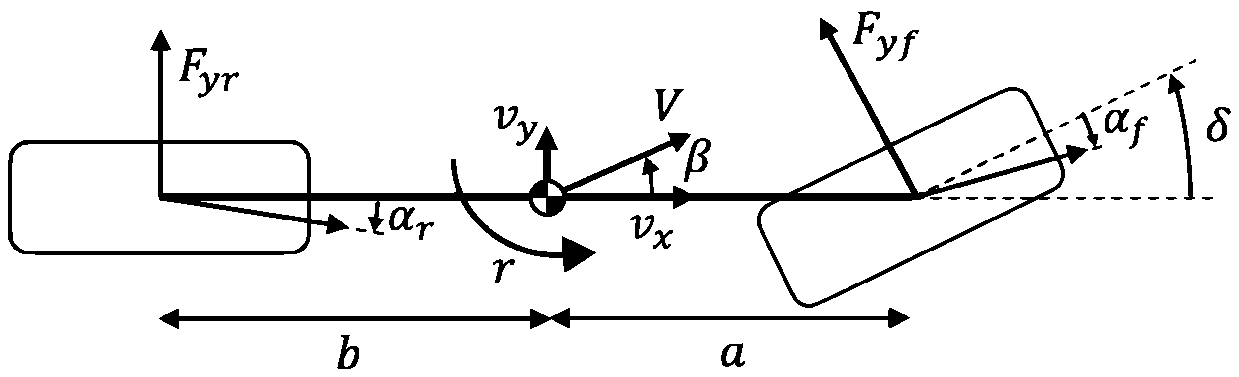
2.1. Dynamic Model

The dynamic extended Kalman Filter approach is based on a nonlinear single track model (see Figure 1). Only lateral and yaw motion are considered:

$$\begin{array}{cc}\hfill {\dot{v}}_y& ={\displaystyle \frac{1}{m}}\left[F_{yf}cos\left(\delta \right)+F_{yr}\right]-v_{x}r\hfill \end{array}$$

(1)

$$\begin{array}{cc}\hfill \dot{r}& ={\displaystyle \frac{1}{I_{zz}}}\left[a{F}_{yf}cos\left(\delta \right)-b{F}_{yr}\right]\hfill \end{array}$$

(2)

Lateral velocity, $v_y$, and yaw rate, r, are the two state variables, while steering angle, $\delta$, and longitudinal velocity, $v_x$, are considered to be the input to the system.

$$\begin{array}{cc}\hfill {\dot{\mathbf{x}}}^{dyn}& =f({\mathbf{x}}^{dyn},{\mathbf{u}}^{dyn})\hfill \\ \hfill {\mathbf{x}}^{dyn}& =\left[\begin{array}{c}{v}_y\\ r\end{array}\right],{\mathbf{u}}^{dyn}=\left[\begin{array}{c}{v}_x\\ \delta \end{array}\right]\hfill \end{array}$$

(3)

m represents the vehicle mass, $I_{zz}$ the yaw inertia and a, b the distance of front and rear axles from vehicle center of gravity (CoG). Sideslip angle is computed from the estimated lateral velocity and from the longitudinal velocity:

$$\beta =arctan\left({\displaystyle \frac{v_y}{v_x}}\right)$$

(4)

The longitudinal velocity is obtained from the average of the measured longitudinal velocities from the four corners

$$v_{x,meas}={\displaystyle \frac{1}{4}}\sum _{i=1}^4{v}_{crn,i}$$

(5)

where $v_{crn,i}$ is the longitudinal velocity at the four corners ($i=1,2,3,4$; $1=$ front left, $2=$ front right, $3=$ rear left and $4=$ rear right). It is computed from wheel speeds, $v_{wheel,i}$, considering also the contribution of steering (only at front) and yaw rate:

$$\begin{array}{cc}\hfill v_{crn,1}& =v_{wheel,1}cos\left(\delta \right)+r{\displaystyle \frac{t_f}{2}}\hfill \\ \hfill v_{crn,2}& =v_{wheel,2}cos\left(\delta \right)-r{\displaystyle \frac{t_f}{2}}\hfill \\ \hfill v_{crn,3}& =v_{wheel,3}+r{\displaystyle \frac{t_r}{2}}\hfill \\ \hfill v_{crn,4}& =v_{wheel,4}-r{\displaystyle \frac{t_r}{2}}\hfill \end{array}$$

(6)

where $t_f$ and $t_r$ are the front and rear tracks, respectively. Longitudinal tyre forces are neglected, while front and rear lateral tyre characteristics are modelled using a customised tyre model, replicating the typical nonlinear behaviour [17]:

$$F_y=\mu F_{z}tanh\left({\displaystyle \frac{C_y}{\mu F_z}}\alpha \right)$$

(7)

where $\mu$ is the tyre–road friction coefficient, $F_z$ is the vertical load, $C_y$ is the cornering stiffness and $\alpha$ the tyre slip angle. $F_z$ is considered to be the static load acting on the two axles, namely $F_{zf}=mg{\displaystyle \frac{b}{l}}=7984\mathrm{N}$ at the front and $F_{zr}=mg{\displaystyle \frac{a}{l}}=6976\mathrm{N}$ at the rear, where l is the wheelbase of the vehicle.

The experimental results, obtained through the procedure detailed in Section 3.2, are fitted with Equation (7) to compute front and rear cornering stiffness and friction coefficient (reported in

Table 1. Alfa Romeo Giulia main parameters.

Parameter	Symbol	Value
Mass	m	1525 kg
Yaw moment of inertia	$I_{zz}$	2130 kg m2
COG to front axle distance	a	1.315 m
COG to rear axle distance	b	1.505 m
Front track	$t_f$	1.557 m
Rear track	$t_r$	1.625 m
Front cornering stiffness	$C_{\alpha f}$	115 kN/rad
Rear cornering stiffness	$C_{\alpha r}$	165 kN/rad
Tyre-road friction coefficient	$\mu$	0.9

), with the results depicted in Figure 2.

The system model in (3) is discretised using the Euler approximation to apply the equations of the discrete-time extended Kalman Filter:

$${\mathbf{x}}_k^{dyn}=f({\mathbf{x}}_{k-1}^{dyn},{\mathbf{u}}_{k-1}^{dyn})\Delta t+{\mathbf{x}}_{k-1}^{dyn}=f_{k-1}({\mathbf{x}}_{k-1}^{dyn},{\mathbf{u}}_{k-1}^{dyn})$$

(8)

where $\Delta t=0.01\mathrm{s}$ is the discretisation interval. The considered measures are the yaw rate and the lateral acceleration. Consequently, the measurement equations may be written as follows:

$${\mathbf{y}}_k^{dyn}=\left[\begin{array}{c}{r}_{meas}\\ a_{y,meas}\end{array}\right]=\left[\begin{array}{c}{r}_k\\ {\displaystyle \frac{F_{yf}cos\left({\delta }_k\right)+F_{yr}}{m}}\end{array}\right]=h_k({\mathbf{x}}_k^{dyn},{\mathbf{u}}_k^{dyn})$$

(9)

System and measurement equations and the respective Jacobian matrices are then used to compute the a priori and a posteriori estimates of the EKF.

2.2. Kinematic Model

The kinematic approach considers longitudinal and lateral velocities as state variables and longitudinal and lateral accelerations to be inputs to the system. The state model is composed by the kinematic relations between accelerations and vehicle velocities:

$$\begin{array}{cc}\hfill {\dot{v}}_x& =v_{y}r+a_x\hfill \end{array}$$

(10)

$$\begin{array}{cc}\hfill {\dot{v}}_y& =-v_{x}r+a_y\hfill \end{array}$$

(11)

The kinematic model can be hence written as a continuous-time state-space model

$$\begin{array}{cc}\hfill {\dot{\mathbf{x}}}^{kin}& =\mathrm{F}{\mathbf{x}}^{kin}+\mathrm{G}{\mathbf{u}}^{kin}\hfill \\ \hfill {\mathbf{x}}^{kin}& =\left[\begin{array}{c}{v}_x\\ v_y\end{array}\right],{\mathbf{u}}^{kin}=\left[\begin{array}{c}{a}_x\\ a_y\end{array}\right]\hfill \\ \hfill \mathrm{F}=& \left[\begin{array}{cc}0& r\\ -r& 0\end{array}\right],\mathrm{G}=\left[\begin{array}{cc}1& 0\\ 0& 1\end{array}\right]\hfill \end{array}$$

(12)

and it may be linearised using the forward Euler method:

$${\mathbf{x}}_k^{kin}=(\mathrm{F}\Delta t+\mathrm{I}){\mathbf{x}}_{k-1}^{kin}+\mathrm{G}\Delta t{\mathbf{u}}_{k-1}^{kin}={\mathrm{F}}_{k-1}{\mathbf{x}}_{k-1}^{kin}+{\mathrm{G}}_{k-1}{\mathbf{u}}_{k-1}^{kin}$$

(13)

The longitudinal velocity is the only measurement, obtained from Equation (5).

The measurement equation is straightforwardly obtained and the discrete-time state-space model is hence completely defined:

$$\begin{array}{cc}\hfill {\mathbf{x}}_k^{kin}& ={\mathrm{F}}_{k-1}{\mathbf{x}}_{k-1}^{kin}+{\mathrm{G}}_{k-1}{\mathbf{u}}_{k-1}^{kin}\hfill \\ \hfill {\mathbf{y}}_k^{kin}& =v_{x,meas}={\mathrm{H}}_k{\mathbf{x}}_k^{kin}=\left[\begin{array}{cc}1& 0\end{array}\right]{\mathbf{x}}_k^{kin}\hfill \end{array}$$

(14)

Since the model is linear, it is possible to resort to a canonical Kalman filter approach. Again, the estimate of $\beta$ is computed with Equation (4), but in this case also the longitudinal velocity is estimated by the Kalman filter.

2.3. Combined Dynamic–Kinematic EKF

Kinematic estimators return good predictions of the state variables, but they are affected by observability issues [18]. From the kinematic state-space model in (14) the observability matrix $\mathcal{O}$ may be computed, resulting in that the rank of $\mathcal{O}$ is lower than the dimension of the state vector in (12) when $r=0$. Consequently, the estimation tends to drift away when the vehicle is driving straight. The observability of the linear system can also be studied by applying the Popov–Belevitch–Hautus (PBH) test [19]. Considering a continuous-time state-space model

$$\begin{array}{cc}\hfill \dot{\mathbf{x}}& =\mathrm{F}\mathbf{x}+\mathrm{G}\mathbf{u}\hfill \\ \hfill \mathbf{y}& =\mathrm{H}\mathbf{x}\hfill \end{array}$$

(15)

$$\mathbf{x}\in {\mathbb{R}}^n\mathbf{u}\in {\mathbb{R}}^m\mathbf{y}\in {\mathbb{R}}^p\mathrm{F}\in {\mathbb{R}}^{n\mathrm{x}n}\mathrm{G}\in {\mathbb{R}}^{n\mathrm{x}m}\mathrm{H}\in {\mathbb{R}}^{p\mathrm{x}n}$$

the PBH test states that the system is observable over $\mathbb{R}$ if, and only if

$$\mathrm{rank}\left[\begin{array}{c}\mathrm{F}-\lambda \mathrm{I}\\ \mathrm{H}\end{array}\right]=n,\forall \lambda \in \mathbb{C}$$

(16)

If the PBH test is performed for the kinematic model (14) it is clear that, when $r=0$, the lateral velocity is unobservable:

$$\mathrm{rank}\left[\begin{array}{cc}-\lambda & r\\ -r& -\lambda \\ 1& 0\end{array}\right]=\mathrm{rank}\left[\begin{array}{cc}-\lambda & 0\\ 0& -\lambda \\ 1& 0\end{array}\right]<2,\mathrm{for}\lambda =0$$

(17)

On the other hand, dynamic estimators do not suffer from observability issues, but, unlike kinematic ones, they are strongly problem-dependent, meaning that a good characterisation of vehicle parameters is needed [20].

To exploit the potential and reduce the impact of weaknesses of both methods, a combined dynamic–kinematic EKF approach is proposed. Figure 3 shows a schematic of the combined algorithm. Estimated quantities are distinguished from measured ones by the use of circumflex ${(}^{^})$ and the subscript meas is dropped for the sake of clarity. Both dynamic and kinematic parts have a prediction block—fed with measurements at step $k-1$—and an update block—fed with measurements at step k. The lateral velocity estimate resulting from the dynamic EKF is used as an additional measurement for the update of the kinematic estimation part. Consequently, the measurement equation of the kinematic model becomes the following:

$${\mathbf{y}}_k^{kin}=\left[\begin{array}{c}{v}_x\\ {\widehat{v}}_y^{dyn}\end{array}\right]=\left[\begin{array}{cc}1& 0\\ 0& 1\end{array}\right]{\widehat{\mathbf{x}}}_k^{kin}$$

(18)

This modification improves the observability of the kinematic model, avoiding the estimate to drift during straights. Applying the PBH observability test to the kinematic part of the combined EKF, it results that the model is observable $\forall \lambda$, also when $r=0$:

$$\mathrm{rank}\left[\begin{array}{cc}-\lambda & 0\\ 0& -\lambda \\ 1& 0\\ 0& 1\end{array}\right]=2$$

(19)

The output of the kinematic model is directly fed into the kinematic part for the subsequent estimation step. Moreover, the resulting longitudinal velocity estimation is used as input to the dynamic part, while ${\widehat{v}}_y^{kin}$ and ${\widehat{r}}^{dyn}$ form the state for next prediction in the dynamic part.

The proposed configuration aims at increasing the robustness of kinematic estimators and improving the dynamic estimation, by correcting it with a part that is independent of vehicle parameters. Consequently, by tuning the covariance matrix of measurement noises of the kinematic part, ${\mathrm{R}}^{kin}$, it is possible to define the level of importance of one part with respect to the other.

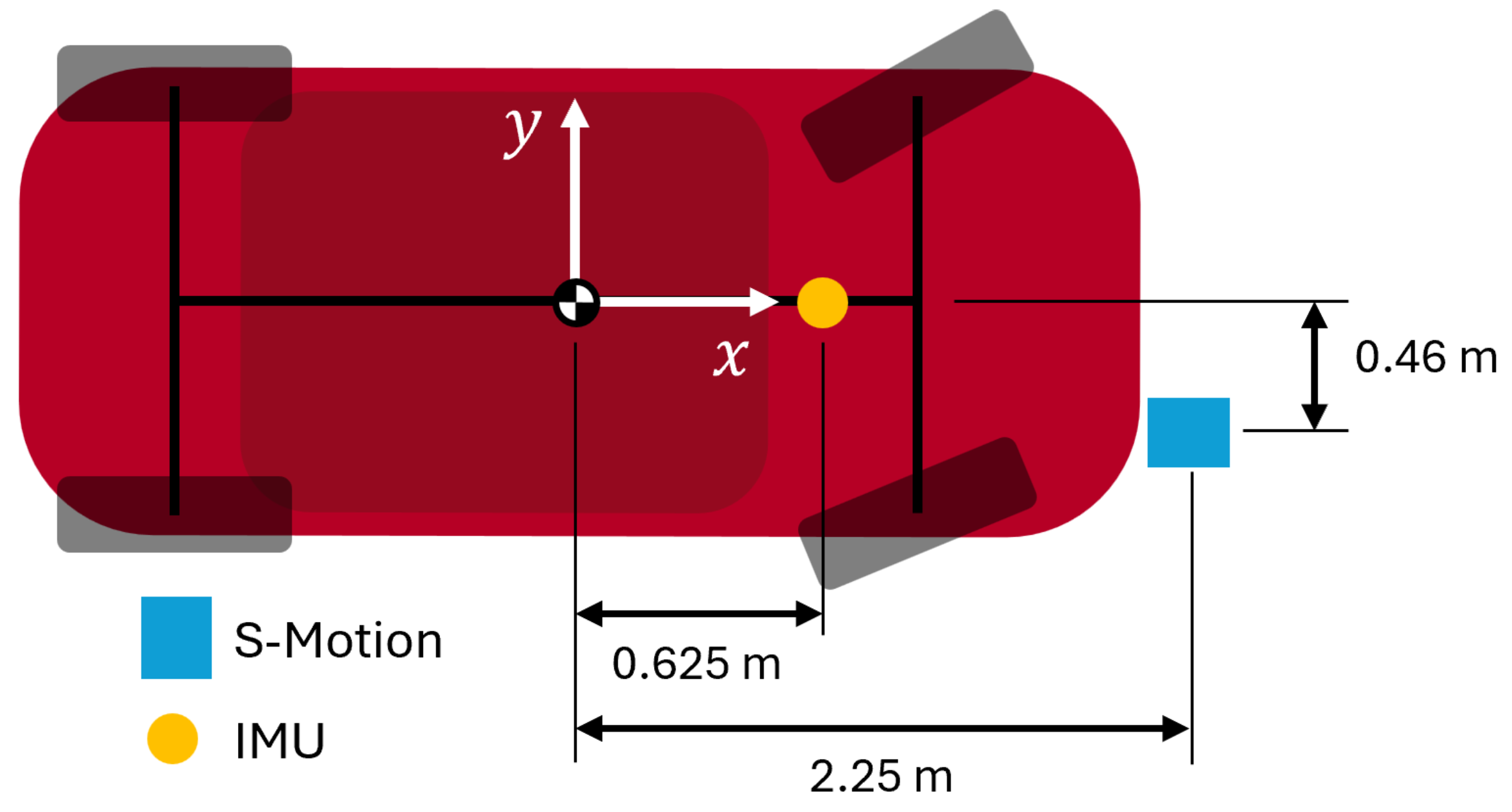
3. Experimental Setup

The combined EKF is validated in a test campaign, conducted at the Mugello Circuit proving ground (Italy). The test vehicle is an Alfa Romeo Giulia, shown in Figure 4. All relevant vehicle parameters are listed in Table 1. The case study instrumentation featured on the vehicle is (Figure 4) as follows:

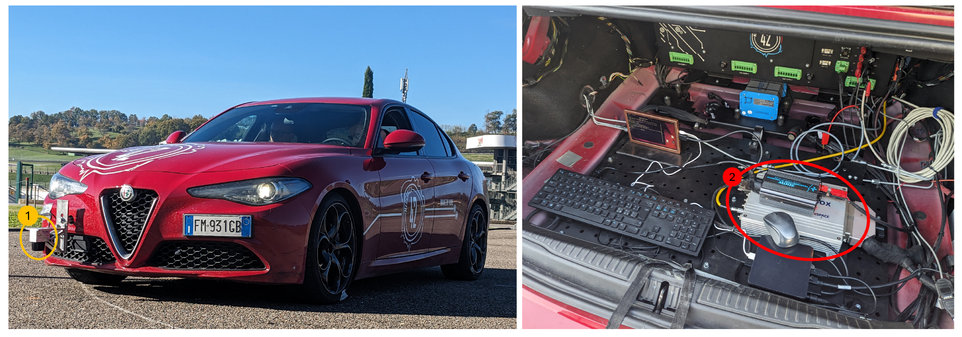
• Kistler Correvit S-motion. It is an optical sensor for measuring the overall vehicle velocity V and the sideslip angle $\beta$. It is herein used to provide a reliable ground-truth comparison.
• dSPACE MicroAutoBox II. It serves as a signal logger, ensuring the synchronization of all recorded signals. Signals logged from the vehicle CAN include accelerations $a_x$, $a_y$, yaw rate r, wheel velocities $v_{wheel,i}$ and the steering angle, $\delta$. Additionally, the dSPACE MicroAutoBox is a powerful real-time system with a high-performance multi-core processor, adept at handling complex control tasks with low latency, making it an excellent candidate for an ECU validation platform.

Double lane change (DLC) and slalom manoeuvres are performed. The first is carried out at a velocity of 50 km/h. Except for the forward velocity, the test parameters are set accordingly to the ISO 3888-2:2011 standard [21]. Figure 5 presents the geometry of the double lane change.

The slalom test is performed at 60 km/h. The manoeuvre consists of going around ten cones at a distance of 20 m between each other [22]. The geometry of the slalom test is outlined in Figure 6. To mark the beginning and end of the manoeuvre, the vehicle must pass through two cones at a distance of 10 m from the first and last cones of the slalom. The manoeuvre is performed at constant speed.

3.1. Signal Pre-Processing

The equations of motion of both dynamic and kinematic approaches, (1), (2) and (10), (11), respectively, are referred as to the vehicle center of gravity (COG). Therefore, it is important to process both input and measurement signals to eliminate undesired effects, moving the signals from the actual measurement location to the COG [23]. Yaw rate is independent from the position of the gyro, while lateral and longitudinal accelerations should be pre-processed according to the location of the vehicle inertial measurement unit (IMU). Assuming planar motion, the acceleration of the center of gravity ${\mathbf{a}}_{COG}$ is computed from the acceleration of any generic point ${\mathbf{a}}_P$ as

$${\mathbf{a}}_{COG}={\mathbf{a}}_P+\dot{r}\mathbf{k}\times \mathbf{PG}-r^2\mathbf{PG}$$

(20)

where $\mathbf{PG}$ is the vector distance of COG from generic point P [24]. Longitudinal and lateral accelerations of the COG are then obtained

$$\begin{array}{cc}\hfill a_x& =a_{P,x}-\dot{r}{\mathrm{PG}}_y-r^2{\mathrm{PG}}_x\hfill \end{array}$$

(21)

$$\begin{array}{cc}\hfill a_y& =a_{P,y}+\dot{r}{\mathrm{PG}}_x-r^2{\mathrm{PG}}_y\hfill \end{array}$$

(22)

where ${\mathbf{a}}_P=a_{P,x}\mathbf{i}+a_{P,y}\mathbf{j}$ and $\mathbf{PG}={\mathrm{PG}}_x\mathbf{i}+{\mathrm{PG}}_y\mathbf{j}$. In the considered case, P corresponds to the location of the vehicle IMU, namely $\mathbf{PG}=(0.625\mathbf{i}+0\mathbf{j})m$.

Similarly, the velocity measured by the Kistler Correvit S-motion should be corrected to obtain the velocity, and hence the sideslip angle, of the COG, in order to have a proper comparison with estimated quantities.

$${\mathbf{v}}_{COG}={\mathbf{v}}_S+r\mathbf{k}\times \mathbf{SG}$$

(23)

Namely

$$\begin{array}{cc}\hfill v_x& =v_{S,x}-r{\mathrm{SG}}_y\hfill \end{array}$$

(24)

$$\begin{array}{cc}\hfill v_y& =v_{S,y}+r{\mathrm{SG}}_x\hfill \end{array}$$

(25)

where ${\mathbf{v}}_S=v_{S,x}\mathbf{i}+v_{S,y}\mathbf{j}$ is the velocity measured at the S-Motion location and $\mathbf{SG}={\mathrm{SG}}_x\mathbf{i}+{\mathrm{SG}}_y\mathbf{j}$ is the vector distance from the COG, namely $\mathbf{SG}=(2.25\mathbf{i}-0.46\mathbf{j})m$. Figure 7 shows a schematic of the test vehicle with the relevant distances depicted.

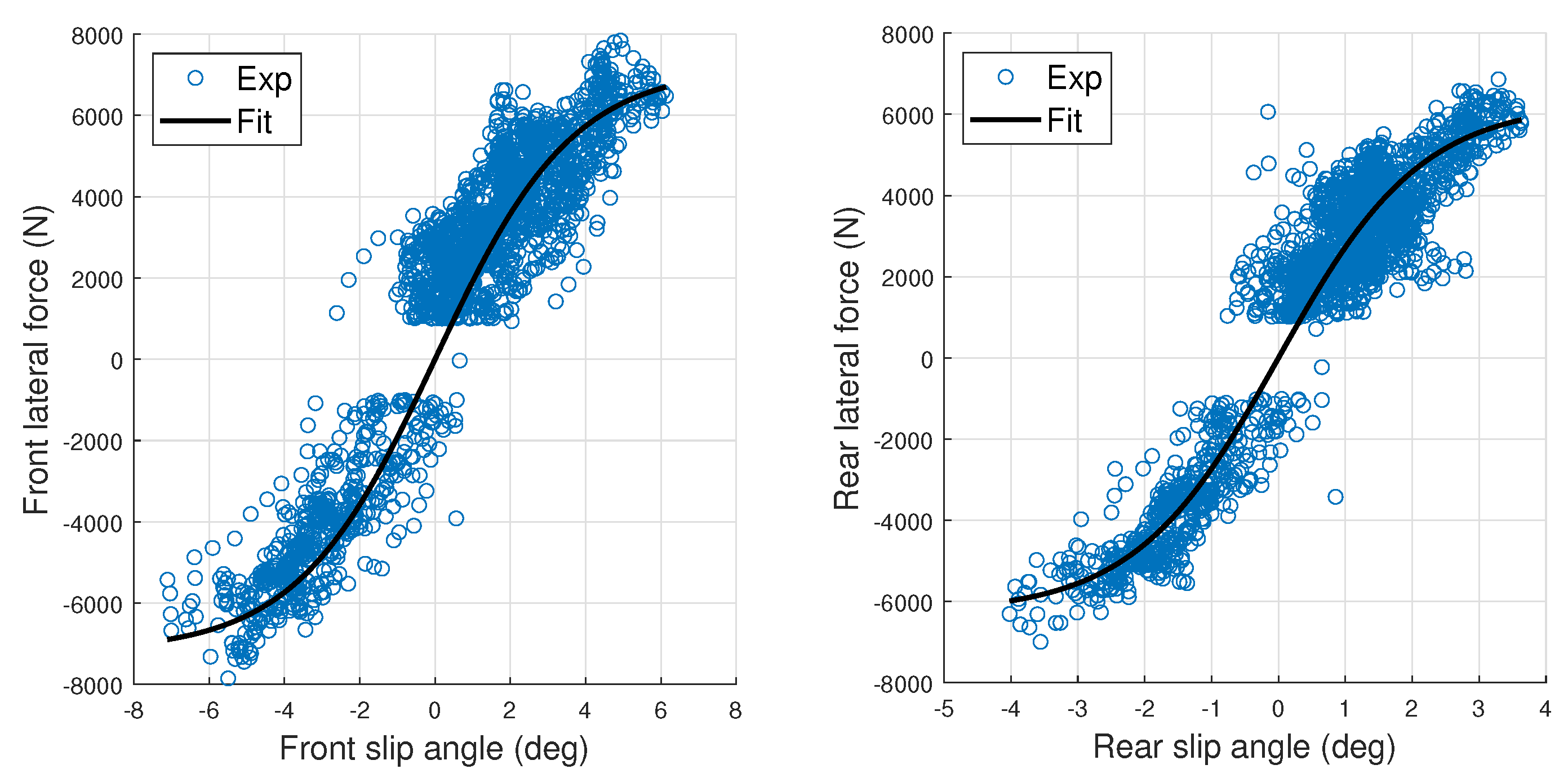
3.2. Experimental Lateral Characteristics of Front and Rear Axles

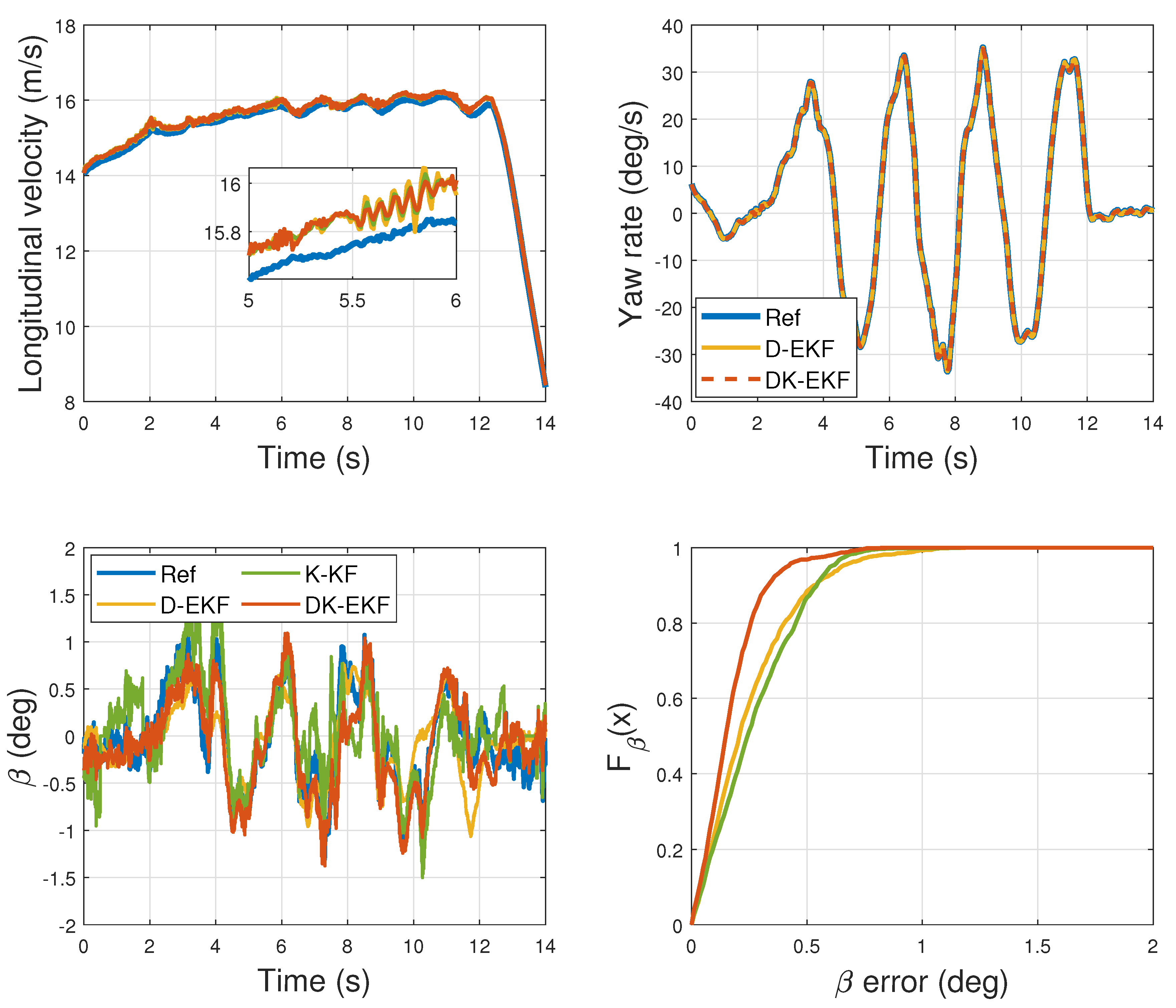
To properly model tyre forces, experimental data are fitted with the tyre model presented in Section 2. Considering the equations of a single track model, front and rear lateral forces are computed by inverting the equations of motion (1) and (2):

$$\begin{array}{cc}\hfill F_{yf}& ={\displaystyle \frac{b}{lcos\delta }}m{a}_y+{\displaystyle \frac{I_{zz}}{lcos\delta }}\dot{r}\hfill \\ \hfill F_{yr}& ={\displaystyle \frac{a}{l}}m{a}_y-{\displaystyle \frac{I_{zz}}{l}}\dot{r}\hfill \end{array}$$

(26)

where $\dot{r}$ is the yaw acceleration, computed by deriving the yaw rate signal using the finite difference approximation.

Front and rear sideslip angles, ${\alpha }_f$ and ${\alpha }_r$ respectively, are computed from steering angle signal, yaw rate signal and longitudinal and lateral velocities:

$$\begin{array}{cc}\hfill {\alpha }_f& =\delta -arctan\left({\displaystyle \frac{v_y+ra}{v_x}}\right)\hfill \\ \hfill {\alpha }_r& =-arctan\left({\displaystyle \frac{v_y-rb}{v_x}}\right)\hfill \end{array}$$

(27)

Data are collected during different driving scenarios of the test vehicle in a previous test session.

4. Results

The performance of the combined DK-EKF is compared to an extended Kalman filter composed by the dynamic part alone (D-EKF), and to a kinematic Kalman filter (K-KF). As is well-known, the performance of Kalman filter estimators depends on the choice of process noise and measurement noise covariance matrices, $\mathrm{Q}$ and $\mathrm{R}$, respectively [25]. The $\mathrm{R}$ matrix contains the variances of sensor noise, while $\mathrm{Q}$ is tuned during the estimator implementation [26]. Since the combined DK-EKF is composed by one dynamic EKF and one kinematic KF, it is necessary to define two pairs of $\mathrm{Q}$, $\mathrm{R}$. The following covariance matrices are selected for the dynamic part:

$$\begin{array}{cc}\hfill {\mathrm{Q}}_{DK}^{dyn}& =\left[\begin{array}{cc}{q}_{v_y}^{dyn}& 0\\ 0& q_r^{dyn}\end{array}\right]=\left[\begin{array}{cc}3·{10}^{-6}{(\mathrm{m}/\mathrm{s})}^2& 0\\ 0& {10}^{-6}{(\mathrm{rad}/\mathrm{s})}^2\end{array}\right]\hfill \\ \hfill {\mathrm{R}}_{DK}^{dyn}& =\left[\begin{array}{cc}{r}_r^{dyn}& 0\\ 0& r_{a_y}^{dyn}\end{array}\right]=\left[\begin{array}{cc}4·{10}^{-7}{(\mathrm{rad}/\mathrm{s})}^2& 0\\ 0& 6·{10}^{-2}{(\mathrm{m}/{\mathrm{s}}^2)}^2\end{array}\right]\hfill \end{array}$$

(28)

and, for the kinematic part

$$\begin{array}{cc}\hfill {\mathrm{Q}}_{DK}^{kin}& =\left[\begin{array}{cc}{q}_{v_x}^{kin}& 0\\ 0& q_{v_y}^{kin}\end{array}\right]=\left[\begin{array}{cc}5·{10}^{-3}{(\mathrm{m}/\mathrm{s})}^2& 0\\ 0& p_{v_y,k}^{dyn}·{10}^{-1}{(\mathrm{m}/\mathrm{s})}^2\end{array}\right]\hfill \\ \hfill {\mathrm{R}}_{DK}^{kin}& =\left[\begin{array}{cc}{r}_{v_x}^{kin}& 0\\ 0& r_{v_y}^{kin}\end{array}\right]=\left[\begin{array}{cc}2·{10}^{-3}{(\mathrm{m}/\mathrm{s})}^2& 0\\ 0& p_{v_y,k}^{dyn}{(\mathrm{m}/\mathrm{s})}^2\end{array}\right]\hfill \end{array}$$

(29)

where $p_{v_y,k}^{dyn}$ is the component related to $v_y$ of the covariance of the estimation error computed by the dynamic part of the filter at time k, $P_k$, that is estimated according to the extended Kalman filter formalism [25]. Since ${\widehat{v}}_y^{dyn}$ is used as a measurement in the kinematic part, but it comes from an estimator rather than an actual sensor, $p_{v_y,k}^{dyn}$ expresses the estimated variance of the signal. Moreover, $q_{v_y}^{kin}$ is set equal to $p_{v_y,k}^{dyn}·{10}^{-1}$ to have a constant ratio $q_{v_y}^{kin}/r_{v_y}^{kin}$. The D-EKF covariance matrices are set equal to the ones in (28), $Q_D=Q_{DK}^{dyn}$, $R_D=R_{DK}^{dyn}$. The covariance matrices of the K-KF are instead different from the ones in (29), since the structure of the filter is also different.

$$\begin{array}{cc}\hfill {\mathrm{Q}}_K& =\left[\begin{array}{cc}5·{10}^{-3}{(\mathrm{m}/\mathrm{s})}^2& 0\\ 0& 3·{10}^{-3}{(\mathrm{m}/\mathrm{s})}^2\end{array}\right]\hfill \\ \hfill {\mathrm{R}}_K& =2·{10}^{-3}{(\mathrm{m}/\mathrm{s})}^2\hfill \end{array}$$

(30)

Moreover, the estimated lateral velocity is set to zero when $\left|r\right|<0.01$ rad/s, to reduce drift during straights.

Figure 8 shows the results of a DLC at 50 km/h. The estimated longitudinal velocity is shown in the top-left plot. For the D-EKF, $v_x$ is not an output of the extended Kalman filter, but it is computed from Equation (5). The three estimations are very similar and close to the reference value (the maximum error is lower than 0.15 m/s), even if all three tend to slightly over-estimate $v_x$. This is due to the averaging of the longitudinal velocities from the four corners, that do not account for longitudinal slips.

Figure 8 also shows the estimation of the yaw rate computed by D-EKF and DK-EKF, compared to the signal of the measured one. Both Kalman filters significantly rely on the measured yaw rate, since the variance of the sensor noise is rather low. The K-KF is not displayed, since it directly uses the measured signal, shown as reference yaw rate. The sideslip angle estimate is presented in the bottom-left plot. The D-EKF is able to predict the general behaviour of $\beta$, but it is not precise. The K-KF estimation is affected by a drifting behavior, but it is better at capturing the high-frequency features of the reference sideslip angle. The DK-EKF corrects the dynamic part and is closer to the reference. Moreover, the kinematic part does not lead to diverging results, thanks to ${\widehat{v}}_y^{dyn}$ entering as a measure.

Table 2. Comparison of RMSE of sideslip angle estimation strategies.

Strategy	DLC	Slalom
D-EKF	0.40 deg	0.33 deg
K-KF	0.60 deg	0.33 deg
DK-EKF	0.27 deg	0.22 deg

reports a comparison of the root mean square error (RMSE) of the $\beta$ estimations, highlighting the higher performance of the DK-EKF, with respect to both D-EKF and K-KF. The cumulative distribution function of the estimation error of $\beta$, $F_{\beta }\left(x\right)$, is also shown in the bottom-right plot of Figure 8. $F_{\beta }\left(x\right)$ expresses the probability that the estimation error of $\beta$ remains below a certain value x, namely $F_{\beta }\left(x\right)=\mathrm{P}(\beta ⩽x)$. This metric clearly shows that DK-EKF outperforms both D-EKF and K-KF, with the latter returning the least reliable estimation.

The results of the slalom manoeuvre are reported in Figure 9. Even in this case, the $\beta$ estimation quality is enhanced by the combined approach, while less significantly. This is confirmed by the difference between the $\beta$ RMSEs (see Table 2). When the D-EKF prediction returns a relevant error, the DK-EKF corrects such behaviour, in general (see, for instance, the predicted sideslip angle between 10 s and 12 s, in the bottom-right plot). The K-KF performs significantly better for the DLC case, due to the high lateral dynamic content of the slalom manoeuvre, as may be seen by looking at the yaw rate signals in the top-right of Figure 9. This is also suggested by the cumulative distribution function of the $\beta$ estimation error, which is very similar to the one of the D-EKF (bottom-right plot of Figure 9). The difference between the RMSE of the DLC and the one of the slalom obtained with the K-KF underlines the weaknesses of this method, due to a drifting behaviour of the estimation when the vehicle lateral dynamics are not sufficiently excited. The RMSEs obtained with the combined approach are instead consistent in the two manoeuvres, highlighting the capability of compensating for the observability issues of the kinematic part of the DK-EKF. Longitudinal velocity signals are again similar and characterised by small errors.

Both test results highlight that the proposed combined approach can give more precise sideslip angle estimation, without displaying drifting of the estimation and effectively compensating for model mismatch. Moreover, the DK-EKF may also be exploited further, by defining variable $Q^{kin}$ and $R^{kin}$ matrices, based on driver inputs. This modification would allow to define how much the estimation relies on the dynamic or on the kinematic part, depending on the current driving condition.

5. Conclusions

This paper presented a novel combined dynamic–kinematic extended Kalman filter (DK-EKF) for vehicle sideslip angle estimation, demonstrating improvements over a dynamic-only extended Kalman filter (D-EKF) and a kinematic-only Kalman filter (K-KF). By integrating both dynamic and kinematic models, the DK-EKF addresses the limitations inherent in each approach, resulting in enhanced estimation accuracy and robustness.

The experimental validation highlights the superior performance of the DK-EKF. During a double lane change (DLC) maneuver at 50 km/h, the DK-EKF accurately predicts lateral velocity, closely aligning with reference values and outperforming both the D-EKF and the K-KF. The root mean square error comparison underscores this improvement, confirming the DK-EKF’s effectiveness in dynamic conditions without diverging results from the kinematic component. In a slalom maneuver, while the improvement is less pronounced, the DK-EKF still demonstrates a corrective influence on the D-EKF’s and K-KF’s predictions. The tendency of the DK-EKF to deviate the dynamic estimation of the lateral velocity when not necessary suggests areas for further refinement.

Overall, the DK-EKF offers a cost-effective accurate solution for real-time sideslip angle estimation, enhancing vehicle stability control systems. Future work will focus on optimizing the DK-EKF’s performance in various driving conditions and further reducing estimation errors, by implementing variable covariance matrices, particularly at higher lateral velocities.

References

1. Bertipaglia, A.; de Mol, D.; Alirezaei, M.; Happee, R.; Shyrokau, B. Model-Based vs Data-Driven Estimation of Vehicle Sideslip Angle and Benefits of Tyre Force Measurements. arXiv 2022, arXiv:2206.15119. [Google Scholar]
2. Melzi, S.; Sabbioni, E. On the vehicle sideslip angle estimation through neural networks: Numerical and experimental results. Mech. Syst. Signal Process. 2011, 25, 2005–2019. [Google Scholar] [CrossRef]
3. Du, X.; Sun, H.; Qian, K.; Li, Y.; Lu, L. A prediction model for vehicle sideslip angle based on neural network. In Proceedings of the 2010 2nd IEEE International Conference on Information and Financial Engineering, Chongqing, China, 17–19 September 2010; IEEE: New York, NY, USA, 2010; pp. 451–455. [Google Scholar]
4. Gurney, K. An Introduction to Neural Networks; CRC Press: Boca Raton, FL, USA, 2018. [Google Scholar]
5. Li, J.; Zhang, J. Vehicle sideslip angle estimation based on hybrid Kalman filter. Math. Probl. Eng. 2016, 2016, 3269142. [Google Scholar] [CrossRef]
6. Ungoren, A.Y.; Peng, H.; Tseng, H. A study on lateral speed estimation methods. Int. J. Veh. Auton. Syst. 2004, 2, 126–144. [Google Scholar] [CrossRef]
7. Chen, B.C.; Hsieh, F.C. Sideslip angle estimation using extended Kalman filter. Veh. Syst. Dyn. 2008, 46, 353–364. [Google Scholar] [CrossRef]
8. Chindamo, D.; Lenzo, B.; Gadola, M. On the vehicle sideslip angle estimation: A literature review of methods, models, and innovations. Appl. Sci. 2018, 8, 355. [Google Scholar] [CrossRef]
9. van Aalst, S.; Naets, F.; Boulkroune, B.; De Nijs, W.; Desmet, W. An adaptive vehicle sideslip estimator for reliable estimation in low and high excitation driving. IFAC-PapersOnLine 2018, 51, 243–248. [Google Scholar] [CrossRef]
10. Naets, F.; van Aalst, S.; Boulkroune, B.; El Ghouti, N.; Desmet, W. Design and experimental validation of a stable two-stage estimator for automotive sideslip angle and tire parameters. IEEE Trans. Veh. Technol. 2017, 66, 9727–9742. [Google Scholar] [CrossRef]
11. Carnier, S.; Corno, M.; Savaresi, S.M. Hybrid Kinematic-Dynamic Sideslip and Friction Estimation. J. Dyn. Syst. Meas. Control. 2023, 145, 051004. [Google Scholar] [CrossRef]
12. Villano, E.; Lenzo, B.; Sakhnevych, A. Cross-combined UKF for vehicle sideslip angle estimation with a modified Dugoff tire model: Design and experimental results. Meccanica 2021, 56, 2653–2668. [Google Scholar] [CrossRef]
13. Ahangarnejad, A.H.; Başlamışlı, S.Ç. Adap-tyre: DEKF filtering for vehicle state estimation based on tyre parameter adaptation. Int. J. Veh. Des. 2016, 71, 52–74. [Google Scholar] [CrossRef]
14. Antonov, S.; Fehn, A.; Kugi, A. Unscented Kalman filter for vehicle state estimation. Veh. Syst. Dyn. 2011, 49, 1497–1520. [Google Scholar] [CrossRef]
15. Zhang, J.; Li, J. Estimation of vehicle speed and tire-road adhesion coefficient by adaptive unscented Kalman filter. J. Xi’an Jiaotong Univ. 2016, 50, 68–75. [Google Scholar]
16. Ren, H.; Chen, S.; Liu, G.; Zheng, K. Vehicle state information estimation with the unscented Kalman filter. Adv. Mech. Eng. 2014, 6, 589397. [Google Scholar] [CrossRef]
17. Righetti, G.; Binetti, E.; de Castro, R.P.; Lot, R.; Massaro, M.; Lenzo, B. On the Investigation of Car Steady-State Cornering Equilibria and Drifting; Technical Report, SAE Technical Paper, Detroit; SAE International: Warrendale, PA, USA, 2024. [Google Scholar]
18. Selmanaj, D.; Corno, M.; Panzani, G.; Savaresi, S.M. Vehicle sideslip estimation: A kinematic based approach. Control. Eng. Pract. 2017, 67, 1–12. [Google Scholar] [CrossRef]
19. Hautus, M.L. Controllability and observability conditions of linear autonomous systems. Ned. Akad. Wet. 1969, 72, 443–448. [Google Scholar]
20. Mosconi, L.; Farroni, F.; Sakhnevych, A.; Timpone, F.; Gerbino, F.S. Adaptive vehicle dynamics state estimator for onboard automotive applications and performance analysis. Veh. Syst. Dyn. 2023, 61, 3244–3268. [Google Scholar] [CrossRef]
21. ISO 3888-2: 2011; Passenger Cars—Test Track for a Severe Lane-Change Manoeuvre—Part 2: Obstacle Avoidance. International Organization for Standardization (ISO): Geneva, Switzerland, 2011.
22. GB/T 6323-2014; Controllability and Stability Test Procedure for Automobile [S]. China Standard Press: Beijing, China, 2014.
23. Selmanaj, D.; Corno, M.; Panzani, G.; Savaresi, S.M. Robust vehicle sideslip estimation based on kinematic considerations. IFAC-PapersOnLine 2017, 50, 14855–14860. [Google Scholar] [CrossRef]
24. Guiggiani, M. The Science of Vehicle Dynamics; Springer: Berlin/Heidelberg, Germany, 2014. [Google Scholar] [CrossRef]
25. Simon, D. Optimal State Estimation: Kalman, H Infinity, and Nonlinear Approaches; John Wiley & Sons: Hoboken, NJ, USA, 2006. [Google Scholar]
26. Madhusudhanan, A.K.; Corno, M.; Holweg, E. Vehicle sideslip estimator using load sensing bearings. Control. Eng. Pract. 2016, 54, 46–57. [Google Scholar] [CrossRef]
Figure 1. Single track model.
Applsci 15 01365 g001
Figure 2. Result of the fitting of the lateral characteristic of the front axle (left) and of the rear axle (right).
Applsci 15 01365 g002
Figure 3. Combined dynamic–kinematic EKF scheme. Subscript (−) and (+) refer to a priori and a posteriori estimates, respectively.
Applsci 15 01365 g003
Figure 4. Vehicle testing setup.
Applsci 15 01365 g004
Figure 5. Geometry of the double lane change.
Applsci 15 01365 g005
Figure 6. Geometry of the slalom test.
Applsci 15 01365 g006
Figure 7. Schematic representation of the position of IMU and S-Motion with respect to vehicle COG.
Applsci 15 01365 g007
Figure 8. DLC at 50 km/h: longitudinal velocity (top-left), yaw rate (top-right), sideslip angle (bottom-left) and cumulative distribution function of β estimation error (bottom-right).
Applsci 15 01365 g008
Figure 9. Slalom at 60 km/h: longitudinal velocity (top-left), yaw rate (top-right), sideslip angle (bottom-left) and cumulative distribution function of β estimation error (bottom-right).
Applsci 15 01365 g009