Predicting Wastewater Characteristics Using Artificial Neural Network and Machine Learning Methods for Enhanced Operation of Oxidation Ditch

Abstract

This study investigates the operational efficiency of the lab-scale oxidation ditch (OD) functioning in simultaneous nitrification and denitrification modes, focusing on forecasting biochemical oxygen demand (BOD₅) concentrations over a five-day horizon. This forecasting capability aims to optimize the operational regime of aeration tanks by adjusting the specific load on organic pollutants through active sludge dosage modulation. A comprehensive statistical analysis was conducted to identify trends and seasonality alongside significant correlations between the forecasted values and various time lags. A total of 20 time lags and the “month” feature were selected as significant predictors. These models employed include Multi-head Attention Gated Recurrent Unit (MAGRU), long short-term memory (LSTM), Autoregressive Integrated Moving Average–Long Short-Term Memory (ARIMA–LSTM), and Prophet and gradient boosting models: CatBoost and XGBoost. Evaluation metrics (Mean Squared Error (MSE), Mean Absolute Error (MAE), Symmetric Mean Absolute Percentage Error (SMAPE), and Coefficient of Determination (R²)) indicated similar performance across models, with ARIMA–LSTM yielding the best results. This architecture effectively captures short-term trends associated with the variability of incoming wastewater. The SMAPE score of 1.052% on test data demonstrates the model’s accuracy and highlights the potential of integrating artificial neural networks (ANN) and machine learning (ML) with mechanistic models for optimizing wastewater treatment processes. However, residual analysis revealed systematic overestimation, necessitating further exploration of significant predictors across various datasets to enhance forecasting quality.

1. Introduction

Machine learning methods (ML) and neural networks (ANN) are increasingly being applied in engineering, particularly in the field of wastewater treatment [1,2,3,4,5]. The primary objectives addressed by these techniques include the development of regression models for predicting water quality [6], minimizing energy consumption [7], and implementing classification models for anomaly detection and preventive maintenance [8].

Machine learning algorithms demonstrate a high level of predictive accuracy when supported by effective data preprocessing, robust validation, and model evaluation practices [9]. In addition to the practical application and fine-tuning of established models, there is growing interest in neural networks whose architectures have been tailored for specific tasks. This includes modifications to the number of neuron layers, the total number of neurons, and their distribution across layers. The architecture of this model, including the number of input and output neurons, is determined by the structure of the input and output data.

In many instances, the internal structure of the network is determined using Kolmogorov’s theory, which employs a hypothetical continuous transformation function. It is essential to conduct experimental validation of the constructed network to verify its parameters. In some cases, algorithms such as the Mezard–Nadal, Marchand, or Lee–Taft methods are suggested for expanding and enhancing the network, while in other situations, techniques for network reduction may be applied.

Sakiewicz [10] developed various neural network configurations to predict biogas production during the anaerobic digestion of wastewater sludge. A total of 18 neural network configurations were examined, including linear networks, multilayer perceptrons (MLP), radial basis function networks (RBF), and general regression neural networks (GRNN). These neural network structures were trained using several algorithms: backpropagation (BP); conjugate gradient (CG); K-means (a training algorithm for radial basis neurons); K-nearest neighbors (KN) for deviation radius determination, pseudoinversion (PI) for linear optimization of least squares errors, and subsample (SS) training algorithms. The linear networks were specifically trained using the PI algorithm. This study identified the operational parameters of the anaerobic digestion unit that significantly influenced the model’s performance, primarily focusing on the technological parameters of the equipment. In contrast, the characteristics of the incoming wastewater had the least impact and were considered uncontrolled parameters. Consequently, a model was developed that enables the optimization of the process through the adjustment of technological parameters.

Jawad [11] investigates the applicability of various neural network architectures in membrane wastewater treatment and seawater desalination. That study highlights the most common neural network architectures, including multilayer perceptrons (MLP), radial basis function networks (RBF), recurrent neural networks (RNN), bootstrap aggregated neural networks (BANN), radial basis function neural networks (RBFNN), Elman neural networks (ENN), and deep neural networks (DNN). The applicability of these neural networks is classified according to the type of primary technological processes: microfiltration; ultrafiltration; nanofiltration; and reverse osmosis. Among these, the MLP architecture remains the most widely used, demonstrating stable performance while still leaving room for improvement in prediction accuracy.

Warren-Vega [12] utilized a neural network to predict the efficacy of advanced oxidation processes (AOP), specifically Fenton and SPF technologies. The neural network produced multiple outputs, allowing for a comprehensive assessment of the technology’s cost with high forecasting accuracy metrics. That study employed a multilayer perceptron (MLP) architecture.

In a separate investigation, Waqas [13] combined a neural network with a support vector machine (SVM) to optimize the operation of a novel membrane-rotating biological contactor (MRBC). This research implemented a neural network utilizing a backpropagation training algorithm based on the Levenberg–Marquardt model, which employs a Gauss–Newton approach. Backpropagation is a standard method for training neural networks in which neuron weights are adjusted in the reverse direction based on the error between the expected and actual outputs of the network. This process is a crucial component of the training algorithm, aimed at minimizing error through gradient descent techniques. The Levenberg–Marquardt model is a numerical method employed for solving optimization problems, particularly in nonlinear regression [14]. This method combines two approaches: the gradient descent method, which is applied when the optimization surface deviates significantly from a quadratic form, and the Gauss–Newton method, which is effective for problems where the optimization surface is close to quadratic.

The Levenberg–Marquardt model adapts its optimization steps by combining both methods: gradient descent is employed when the gradients vary significantly, while the Gauss–Newton method is used when the error is approximately linear (nearly quadratic) [15]. In the course of this study, a model was developed to optimize key technological parameters, including the rotation speed of the disk, hydraulic retention time (HRT), and the solid retention time (SRT) of activated sludge in the reactor. The coefficient of determination exceeded 0.9 on the test data, indicating a strong correlation between this model and real operating conditions.

Ranade [16] trained a similar model to refine the characteristics of sludge pretreatment, achieving an R² value exceeding 0.99. Models utilizing backpropagation have also been explored by researchers under the guidance of Sibiya [17]. They developed a model with one hidden layer containing 20 neurons and an output layer with 4 neurons to predict the efficiency of wastewater treatment in rice farming. The model’s performance was assessed using the coefficient of determination, which yielded a value of 0.9935. Similarly, Wang [18] obtained comparable results with a similarly structured model for predicting the efficiency of advanced wastewater treatment using coagulants, flocculants, and magnetic powder.

In the previously discussed studies, the modeling approach was based on the premise that the datasets did not represent ordered time series. Consequently, the developed neural networks were applied to datasets without considering trend analysis. However, there is considerable interest in the application of neural networks, specifically to time series data. These networks enable the effective implementation of “soft sensors” that provide information on water quality at various treatment facility nodes, predicted based on incoming wastewater data while accounting for daily and seasonal variability. Several classes of specialized neural networks are suitable for these purposes. One notable example is the long short-term memory artificial neural network (LSTM). LSTM is a type of artificial neural network that belongs to the class of recurrent neural networks (RNNs) and is specifically designed for processing and analyzing sequential data. LSTMs are particularly useful for working with data that exhibit temporal dependencies, such as time series, text, or sequential events. The primary advantage of LSTM networks lies in their ability to retain critical information over extended periods while disregarding less significant data. Components of LSTM include a Memory Cell, the fundamental unit responsible for storing information and managing its retention, updating, and deletion; an Input Block, which determines which portions of new information will be added to the memory; a Forget Gate, which regulates what information will be discarded from the memory; and an Output Block, which specifies which part of the stored information will be utilized for the current output.

Xu [19] trained an LSTM model using data from a laboratory A/O bioreactor and compared its performance with that of a multifactorial linear regression model. The mean absolute percentage error (MAPE) was used as the target metric. On average, the LSTM model demonstrated significantly higher forecasting accuracy across three indicators, with a difference of up to 30%. Farhi [20] explored a model that predicted anomalous levels of ammonia and nitrates in treated wastewater during seasonal temperature fluctuations. An LSTM Auto-Encoder was employed in this study. This model is trained on normal data, where the input sequence is fed into the LSTM encoder, compressed into a latent space, and then reconstructed by a decoder. The objective is to minimize the reconstruction error. When processing new sequences, anomalous data generate a higher reconstruction error, allowing for the detection of deviations from normal patterns. The inclusion of the encoder led to improved performance compared to traditional LSTM models, potentially due to the application of various time-processing techniques, such as different window aggregations, steps, and sizes. The effectiveness of using autoencoders in conjunction with LSTM models is supported by several contemporary studies [21,22,23].

Another widely used neural network architecture for working with time series data is the Multi-Attention Gated Recurrent Unit (MAGRU). This architecture combines an attention mechanism with a modified version of the Gated Recurrent Unit (GRU), making it suitable for tasks that require sequential data processing. Safder [24] utilized networks of this architecture to monitor wastewater treatment parameters at a facility in South Korea, achieving greater accuracy compared to other neural networks as evaluated by the Mean Absolute Error (MAE). On average, MAGRU demonstrated accuracy metrics that were 15–20% higher than those of other models employed in this study. These findings are corroborated by additional sources [25,26,27]. Overall, it can be observed that hybrid models tend to be the most effective in comparative studies, providing a flexible approach to data handling. Notable examples include the Complete Sliding Window LSTM Gaussian Process Regression (CSWLSTM-GPR) [28], AutoRegressive Integrated Moving Average–LSTM (ARIMA–LSTM) [29], and LSTM with Genetic Algorithm (GA–LSTM) [30], among others.

The study by Wang [31] addresses critical challenges in multivariate time series regression by proposing a novel nonlinear function-on-function model. Unlike conventional approaches, such as multivariate regression models and Seq2Seq architectures, which are limited by their inability to handle irregular time series and temporal dependencies, the proposed method leverages fully connected neural networks to capture complex correlations. This model integrates and extends the function-on-function linear model, addressing issues of bias, inefficiency, and underfitting commonly associated with traditional methods. The effectiveness of this approach is validated through applications to real-world datasets, demonstrating its potential to significantly enhance predictive accuracy in time series analysis. This contribution represents a significant advancement in functional data analysis and time series modeling, offering robust solutions for diverse applications.

This study investigates the performance of neural networks, specifically MAGRU, LSTM, ARIMA–LSTM, and Prophet, for forecasting the operation of the oxidation ditch (OD) under the simultaneous nitrification and denitrification (SND) technology. While current research on the application of neural networks in modeling OD operations is ongoing [32,33,34], few studies specifically focus on optimizing the SND process [35]. This work explores the potential for forecasting the inflow of organic pollutants, which exhibit pronounced trends and seasonality, to regulate the load on activated sludge and optimize system performance. Given that measuring BOD₅ levels in laboratory conditions takes a minimum of five days, timely optimization of wastewater treatment plants not equipped with expensive online monitoring systems for organic pollutants poses significant challenges. Forecasting pollutant inflow based on observed trends holds substantial practical value, provided there is a sufficient amount of statistical data available.

2. Materials and Methods

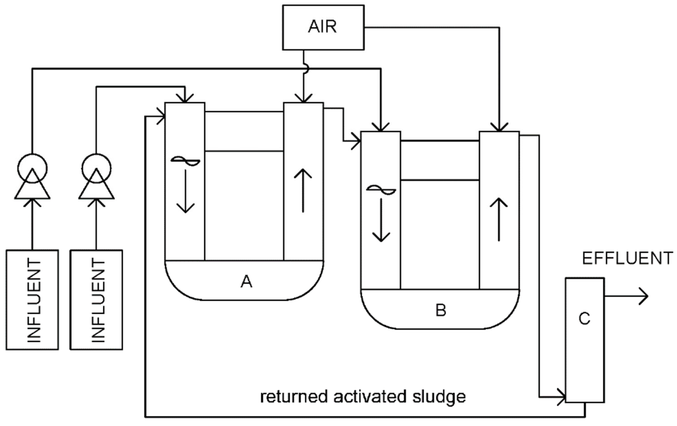
2.1. Experimental Setup

This study examines the operation of the OD employing simultaneous nitrification and denitrification technology. The laboratory setup and its operational principles were detailed in previous works [36]. The laboratory installation consisted of a model OD with vertical flow constructed from polycarbonate tubes with a diameter of 100 mm. It comprised two modules with volumes of 20 and 17 L, respectively. The reactor design ensured ideal mixing across the entire width of the corridor, free from any gravitational influences. The substrate feed rate varied from 4.2 to 7.5 L per hour. The reactor was equipped with a single sedimentation tank with a maximum active volume of 8 L. Synthetic wastewater was introduced into the OD using two solenoid dosing pumps operating in a batch dosing mode (50%/50%). A schematic representation of the setup is shown in Figure 1.

The duration of the experimental phase was 24 months. The data obtained during the experiment are described in Section 2.4. The primary regulated characteristics of the setup included the concentration of dissolved oxygen across different zones (DO, mg/L), hydraulic retention time (HRT, hours), and mixed liquor-suspended solids (MLSS, mg/L). The sludge retention time (SRT) was maintained at 20 days. The MLSS concentration was adjusted by regulating the return-activated sludge flow, which allowed for a constant biochemical oxygen demand (BOD₅) loading of 0.2 g/g/d, as required by the experimental conditions. In accordance with the BOD₅ concentration in the incoming wastewater, the dissolved oxygen levels in the individual bioreactor zones were also adjusted. In the first zone (A), the oxygen concentration varied from 0.1 mg/L to 0.5 mg/L, while in the second zone (B), it ranged from 0.35 mg/L to 0.8 mg/L. The HRT varied between 6.5 h and 12 h. The flow rate in the oxidation ditch was maintained at 0.2 m/s. A detailed description of the setup can be found in a previous study [36]. The primary focus of this research is the analysis of time series data reflecting the changing concentration of biochemical oxygen demand (BOD₅, mgO₂/L).

2.2. Chemicals

In this study, reagents of analytical grade were utilized, which were suitable for use without further purification. These included reagents from VWR International LTD (Leicestershire, UK), such as ammonium chloride (NH₄Cl, AnalaR NORMAPUR, 99%), potassium dihydrogen phosphate (KH₂PO₄, AnalaR NORMAPUR, 99.5%), sodium acetate (CH₃COONa, AnalaR NORMAPUR, 99%), meat peptone (enzymatic hydrolysate), and ethanol (CH₃CH₂OH, absolute TechniSolv, 99.5% purity).

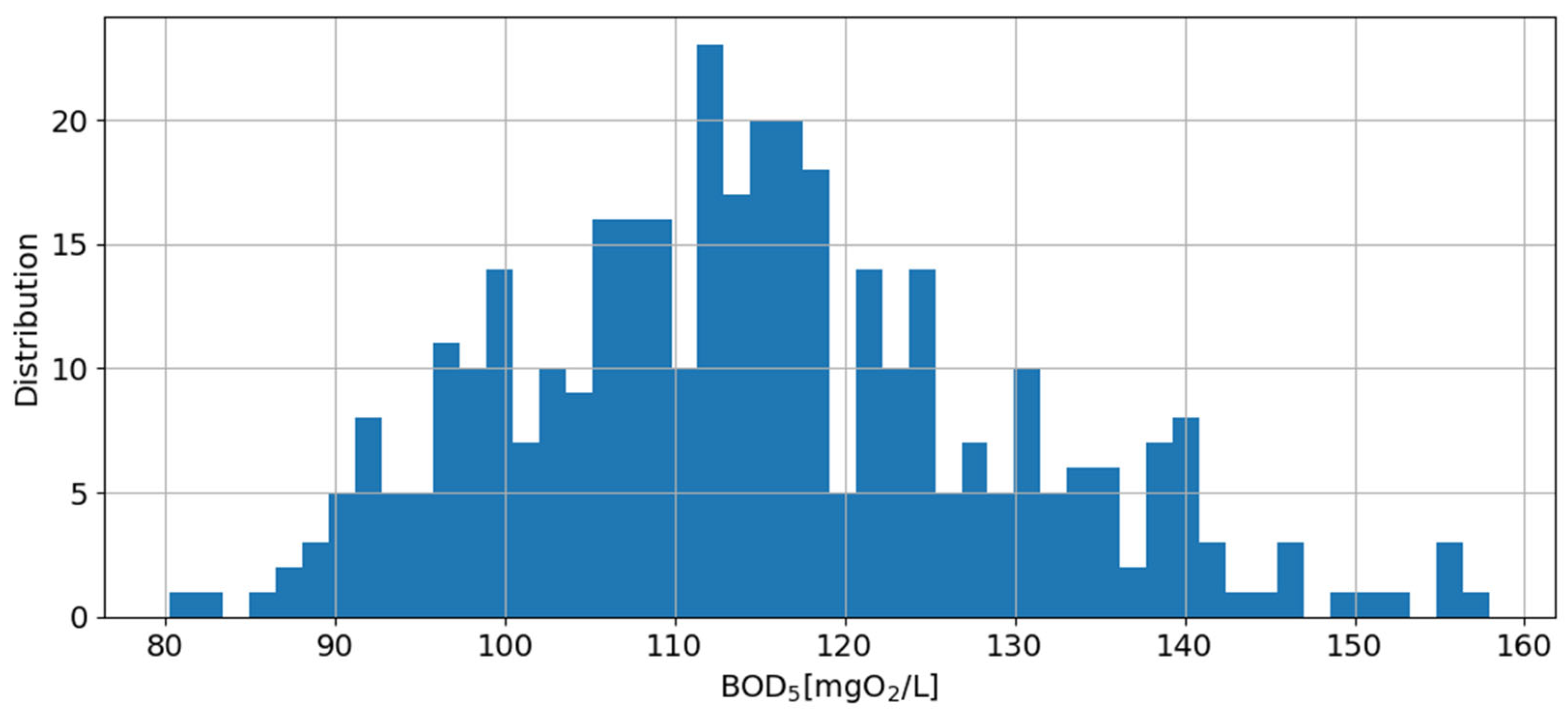
2.3. Wastewater Characteristics

This study was conducted using synthetic wastewater resembling the composition of wastewater from the Moscow region in Russia. The synthetic wastewater was prepared based on dry peptone, containing 1.8 ± 0.75 g/L of peptone, 0.05 ± 0.02 g/L of NH₄Cl, 0.08 ± 0.03 g/L of NaCH₃COO, and 0.02 ± 0.008 g/L of KH₂PO₄. If necessary, the ratio of biodegradable organic matter in the wastewater was adjusted by adding ethanol (1.0 ± 0.5 mL/L). During this study, the concentrations in the wastewater varied according to the experimental program and are presented within the ranges shown in

Table 1. Concentrations of synthetic wastewater.

Parameter	Max.	Min.	Mean
BOD5, mgO2/L	158	80	115
NH4-N, mg/L	81.8	18.5	37
PO4-P, mg/L	13.5	2.8	7.2
TSS, mg/L	194.15	89.88	115.36
pH	8.7	7.3	7.7

.

The variations in contaminant concentrations occurred in accordance with the seasonal and diurnal cycles typical of wastewater received at treatment facilities in the Moscow region. These fluctuations are influenced by irregularities in water usage and environmental conditions, such as pipeline infiltration, seasonal agricultural activities, and other factors. A detailed description of the time series is provided in Section 2.4.

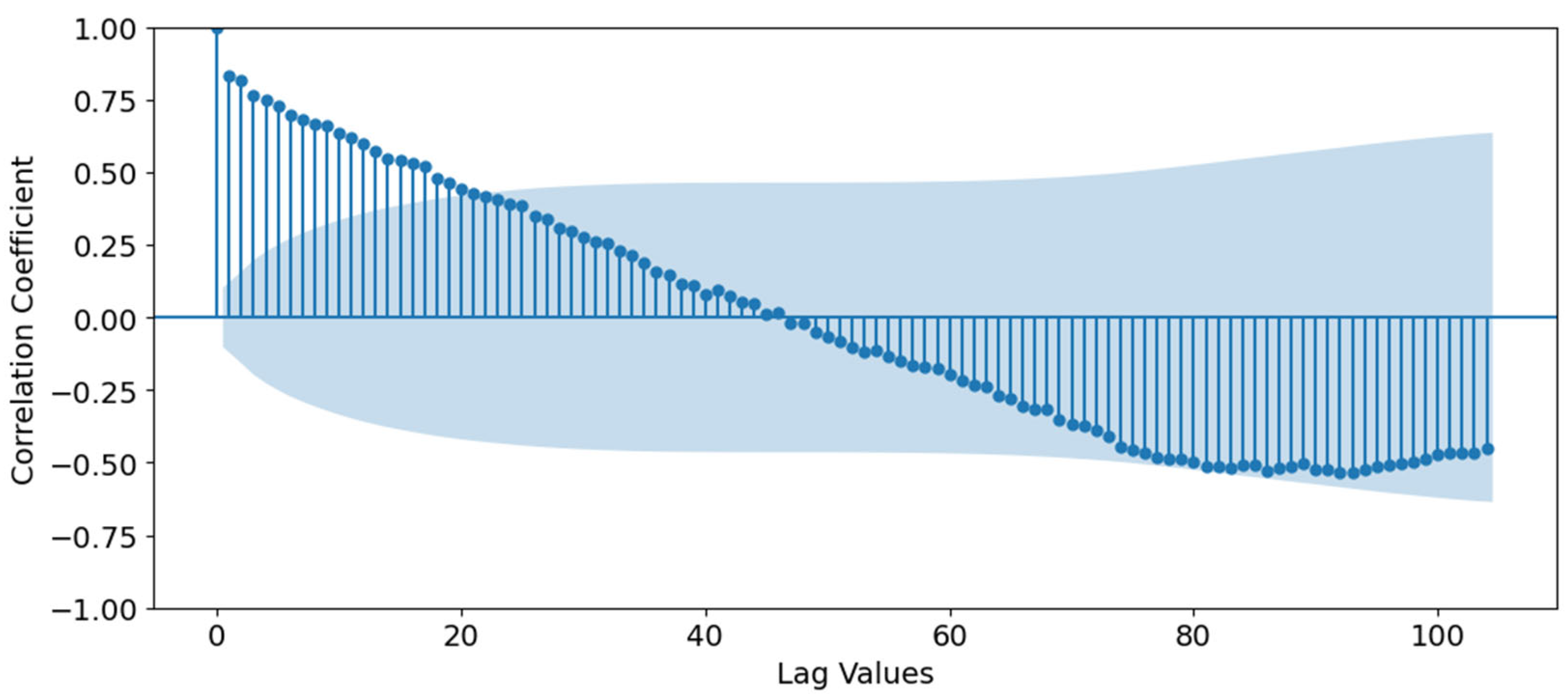
2.4. Data Description and Analysis

This study focuses on modeling the characteristics of incoming wastewater based on a single time series (BOD₅ values, mgO₂/L). This research was conducted over a period of 24 months, during which BOD₅ measurements were taken every two days, resulting in a total of 327 analytical results. Figure 2 illustrates the graphs depicting the distribution of these values.

The distribution of the values is normal, as confirmed by the Shapiro–Wilk test. There are no long tails present, and the values fall within the ranges established by the experimental program. The collected data contain a small number of outliers that fall beyond 1.5 times the interquartile range (IQR). These outliers correspond to peak substrate concentrations and are not considered anomalous. Therefore, no data correction is necessary. Figure 3 displays the time series of the obtained data.

Figure 4 illustrates the values of BOD₅ after resampling. The resampling was conducted using the weekly average, which facilitates the interpretation of the timeline.

Figure 5 presents the trend and seasonal component graphs for the studied timeline. It is evident that the values exhibit a pronounced trend and seasonal component, which will be utilized during the training of the neural network. The upward trend indicates an increase in BOD₅ concentration, which is associated with the implementation of water-saving technologies in the region under study. The seasonality of pollutant concentrations is attributed to the dilution of wastewater due to groundwater infiltration in the sewage systems. Additionally, the summer months in the region are characterized by low precipitation, which further impacts wastewater concentrations, particularly due to the inflow of stormwater into the municipal sewer system.

Figure 6 presents the Autocorrelation Function (ACF) plot for the non-resampled data. Based on the area of statistical significance, lag values exhibiting positive correlation and identified as statistically significant can be observed up to 20 lags. These lags were used as predictors in the modeling process. Additionally, the variable “month” was included as a predictor due to the evident correlation between the month of observation and the average value of the indicator. Furthermore, a “rolling” average was introduced, representing the moving average (the mean BOD₅ value over the most recent measurements, in this case, three measurements).

Thus, the dataset for modeling comprised 22 predictors, one target variable, and 327 data rows. The training set constituted 80% of the total data, while the test set accounted for 20%. The data were provided to these models without shuffling.

2.5. Methodology

Modeling was conducted using neural networks whose architectures are recommended for time series analysis: MAGRU; LSTM; and ARIMA–LSTM. The parameters for the LSTM model were selected as follows:

• First Layer: An LSTM layer with 50 units and the parameter “return_sequences = True”, allowing the sequences to be passed to subsequent layers;
• Dropout Layer: Following the first LSTM layer, a Dropout layer was applied with a neuron dropout rate of 20% (0.2) to prevent overfitting;
• Second Layer: Another LSTM layer with 50 units, where “return_sequences = False”, ensuring that only the final output sequence is passed to the next layer;
• Second Dropout Layer: Another Dropout layer with a 20% probability of stabilizing the training process;
• Dense Layer: A fully connected (Dense) layer with 25 neurons to provide additional representation and transformation of features following the LSTM layers;
• Output Layer: A final Dense layer with one neuron for predicting the target value, as the task involves forecasting a single output parameter;
• Compilation: This model was compiled using the Adam optimizer and the Mean Squared Error (MSE) loss function, which ensured the optimization of prediction accuracy for regression tasks;
• Training Parameters: A batch size of 32 samples and 100 epochs were selected for model training. The data were divided into training and testing sets in an 80/20 ratio using the “train_test_split” function. This model was trained on the training set, while the quality was assessed on the testing set;
• Normalization: All input features and target values were normalized to a range of 0 to 1 using “MinMaxScaler” to enhance the quality of training.

The potential to enhance the efficiency of the LSTM model through the implementation of a model incorporating an attention mechanism—Multi-head Attention Gated Recurrent Unit (MAGRU)—was explored. This model combines a multi-head attention mechanism with Gated Recurrent Unit (GRU) layers, enabling it to effectively capture both temporal dependencies and the significance of individual features in the data (with significant features being defined as the month of the year in this context) [25,26,27]. The parameters of the MAGRU model are as follows:

• This model begins with a multi-head attention layer featuring four heads. The size of the keys for each head is equal to the number of input features (22), allowing each head to focus on different aspects of the input data. This architecture enables the network to identify important dependencies among features across various time steps, thereby enhancing the extraction of temporal relationships;
• Following the multi-head attention layer, a Dropout layer with a dropout rate of 20% is included to prevent overfitting and improve the model’s generalization capability. Additionally, layer normalization with a small epsilon value (1 × 10⁻⁶) is applied to stabilize the network by normalizing the output of the attention layer;
• This model incorporates a residual connection that adds the original input data to the attention layer’s input. This retains the original representation of the data while complementing it with the attention results to enhance feature characteristics;
• Two consecutive GRU layers, each with 64 units, are utilized for further processing of the temporal sequence. The first GRU layer returns sequences (“return_sequences = True”), while the second GRU layer outputs only the final hidden state. Both GRU layers are accompanied by Dropout layers with a 20% dropout rate to mitigate overfitting;
• After the GRU layers, a fully connected (Dense) layer with 32 neurons and ReLU activation is used to form higher-level representations of the data. This is followed by a Dense output layer with a single neuron to predict the target value;
• This model was compiled using the Adam optimizer and the Mean Squared Error (MSE) loss function. MSE is suitable for regression tasks as it minimizes the mean squared deviation between the predicted and actual values, thereby enhancing forecasting accuracy. To improve model robustness, Dropout is applied after the attention layer and each GRU layer with a probability of 20%. This reduces the likelihood of overfitting, particularly when handling complex temporal data.

Another model considered in this study is ARIMA–LSTM, a hybrid framework that combines the linear ARIMA model with the LSTM neural network [29]. This approach enables the capture of both linear and nonlinear temporal dependencies. This model consists of the following stages:

• In the initial phase, the ARIMA model is applied separately to each feature of the time series. The use of ARIMA facilitates the extraction of trend and seasonal components, highlighting their linear dependencies. The residuals obtained from the ARIMA model for each feature are then calculated, forming a time series that will be further trained in the LSTM neural network. In this study, the parameters of the ARIMA model are empirically selected for each series;
• The typical order of the ARIMA model used for trend analysis was (5, 1, 0), where 5 represents the autoregressive order; 1 indicates the order of differencing, and 0 signifies the order of the moving average;
• In the second phase, the ARIMA residuals are fed into the LSTM neural network to identify remaining nonlinear dependencies. The data were normalized to a range of 0 to 1 using “MinMaxScaler” to accelerate training and enhance the model’s robustness;
• The first LSTM layer consists of 64 units, returning sequences (return_sequences = True) for the subsequent layer. A Dropout layer with a probability of 0.2 is included to prevent overfitting;
• The second LSTM layer also contains 64 units but returns only the final hidden state (“return_sequences = False”);
• A fully connected (Dense) layer with 32 neurons and ReLU activation is applied to enhance nonlinear representations of the data. The output Dense layer contains 22 neurons, corresponding to the number of forecasted features;
• This model was compiled using the Adam optimizer and the Mean Squared Error (MSE) loss function, which is a standard approach for regression tasks. Training was conducted for 100 epochs with a batch size of 32.

In addition, we considered the Prophet model (developed by the Facebook research team) as a comparative baseline [37]. Prophet decomposes time series into trend, seasonality, and holiday components, allowing for easy interpretation and flexible incorporation of domain-specific knowledge. Compared to the MAGRU, LSTM, and ARIMA–LSTM approaches, Prophet tends to excel in handling irregular data frequencies and requires fewer manual adjustments of parameters, but it may struggle to capture complex nonlinear dependencies and long-term temporal patterns. Structurally, Prophet assumes an additive model consisting of a piecewise linear (or logistic) growth trend and multiple seasonalities that can be independently specified. For this study, we configured Prophet with a learning rate of 0.05, a seasonality mode set to “additive”, enabled yearly and weekly seasonalities, and a changepoint prior scale of 0.1 to control trend flexibility. While the relative simplicity and interpretability of Prophet offer valuable advantages, its forecast accuracy may be limited when confronted with intricate time-series dynamics that the more specialized MAGRU, LSTM, and ARIMA–LSTM models are designed to capture.

In addition to the artificial neural network (ANN) models, two gradient-boosting ensemble methods were employed: CatBoost (developed by Yandex) and XGBoost (developed by Chen and Guestrin) [38,39,40]. While both models leverage gradient-boosted decision trees, CatBoost uses ordered boosting and special handling of categorical features, whereas XGBoost primarily focuses on computational efficiency and effective tree pruning. For the CatBoost model, hyperparameters were optimized via cross-validation, resulting in a learning rate of 0.05, 150 iterations, a depth of 7, and a random strength of 2. Similarly, the XGBoost model was tuned with a learning rate of 0.05, 150 boosting rounds, a maximum depth of 7, and a subsample ratio of 0.8 to improve generalization. These configurations were chosen to maximize predictive performance, as determined by the specified evaluation metrics.

Alongside the Mean Squared Error (MSE), other metrics considered for evaluation included the coefficient of determination (R²), Mean Absolute Error (MAE), and Symmetric Mean Absolute Percentage Error (SMAPE).

The performance of time series models such as ARIMA, LSTM, Prophet, and MAGRU has been previously evaluated on various datasets in earlier studies [41,42,43]. In many cases, the predictive accuracy of these models was highly dependent on the nature and characteristics of the data being analyzed, including its complexity, nonlinearity, and seasonality. In this study, we focus on a dataset representative of the time series of influent wastewater quality, which presents unique challenges such as irregular patterns, potential outliers, and noise. By leveraging these models, we aim to determine their relative effectiveness in forecasting wastewater quality parameters and analyze their suitability for this specific application. The comparison provides insights into the adaptability of these models to environmental datasets, characterized by variability and the need for precise predictions to support decision-making in wastewater treatment processes.

3. Results and Discussion

The modeling results demonstrated the capability to achieve stable predictions of BOD₅ values up to 5 days in advance using all the examined models. This forecasting enabled proactive adjustments to the volume of recycled return-activated sludge, thereby regulating the Mixed Liquor Suspended Solids (MLSS) and, consequently, the specific load of organic pollutants. Additionally, adjustments were made to the aeration scheme of the facility and the duration of the treatment process. Direct measurement of BOD₅ using conventional methods within a timeframe shorter than 5 days is impractical; therefore, this forecast holds significant practical value for the operation of wastewater treatment plants. The performance metrics of these models based on the test data are summarized in

Table 2. Metrics for Evaluating Models Performance.

Model	MSE	MAE	SMAPE	R2
LSTM	2.860	1.332	1.183	0.987
ARIMA–LSTM	2.754	1.224	1.052	0.991
MAGRU	2.799	1.289	1.091	0.986
Prophet	3.005	1.417	1.288	0.918
CatBoost	3.011	1.421	1.301	0.897
XGBoost	3.028	1.435	1.312	0.891

.

The performance of these models was consistent. The identified prediction errors were significantly lower than the actual error of the analytical method for determining BOD5, which has a relative error of 9% in the concentration range of 100 to 300 mg/L. The best results were achieved by the ARIMA–LSTM architecture, which effectively accounted for various types of dependencies. Notably, the LSTM model alone also demonstrated high performance and could be used without the ARIMA component, reducing resource consumption. The literature supports the effectiveness of LSTM modeling for predicting values in time series related to the quality of incoming wastewater [19,20,30,44].

The magnitude of the error depends on the characteristics of the time series itself and the presence of necessary correlation dependencies. To improve modeling quality using the MAGRU architecture, it is essential to identify the most significant additional predictors for inclusion in this model. In this study, the “month” characteristic was used, indicating an overall trend of increasing or decreasing concentrations of the target variable. Additional predictors are described in works [12,28,45,46] and should be integrated into the monitoring system at the stage of time series formation.

Additionally, the ensemble models CatBoost and XGBoost also demonstrated high accuracy. Their metrics were nearly identical, which can be attributed to the dataset being equally well-suited for both models. This is supported by recent studies that examined the results of these models in time series tasks related to wastewater characteristics [47,48,49]. At the same time, the Prophet model showed weaker results compared to more specialized models. However, its performance can still be considered acceptable within the scope of the studied task. Prophet’s ability to handle time series with simple seasonality makes it a useful tool for preliminary data analysis [50].

All models under consideration—LSTM, ARIMA–LSTM, MAGRU, Prophet, CatBoost, and XGBoost—incorporated the additional predictor, “month”, allowing them to capture temporal patterns associated with monthly variations. Notably, if a pure ARIMA model had also been considered, it would not have been able to accommodate this additional predictor due to its inherent limitations in handling multiple input features. By including “month” as a predictor, we aimed to represent the seasonal and trend-related aspects that arise over the course of a year. This encompasses not only the cyclical changes in wastewater inflow and concentrations but also the gradual upward trend in key parameters. Moreover, the differences in relative values observed across various months—established through both prior data analysis and laboratory-scale experiments—were effectively modeled by these approaches. As a result, the inclusion of the “month” variable enabled the selected methods to better capture monthly seasonality, improving the overall accuracy and interpretability of the time series forecasts.

Figure 7 illustrates the graph depicting the distribution of actual and predicted values of the target variable.

It is evident that the prediction accuracy is predominantly high. To further assess the model’s performance, a residual analysis was conducted. The graphical representation of this analysis is shown in Figure 8.

Since the median of the residuals is shifted away from zero, this may indicate the presence of systematic error—this model slightly overestimates values, as suggested by the slightly elongated left tail. Additionally, the linear relationship describing the residual scatter has a low coefficient of determination, which can be interpreted as a sign of the absence of dependency. Neither overfitting nor underfitting of this model is clearly indicated. However, it is evident that the model’s accuracy can be improved. As previously mentioned and discussed in the literature, the most effective approach to achieving this is to introduce new significant predictors into this model. Future studies will focus on selecting predictor sets for both time series modeling and regression tasks, utilizing SHapley Additive exPlanations (SHAP) analysis [44].

Based on the predicted BOD₅ concentrations, adjustments to the activated sludge dosing were carried out by modifying the ratio of return sludge to excess sludge in the physical model. Since the characteristics of the substrate used imply a nonlinear relationship between COD and BOD₅, direct measurement of BOD₅ was not feasible. This limitation made it difficult to promptly adjust the specific organic loading rates, as such adjustments had previously been performed five days after wastewater introduction—corresponding to the conventional five-day BOD₅ incubation period required for this analysis.

To overcome these challenges, machine learning approaches were employed to refine wastewater characteristics in advance. By enabling preventive control of key operational parameters, these predictive methods enhanced overall system stability. As a result, no emergency conditions arose during subsequent model operations. In particular, the system exhibited no filamentous bulking of the activated sludge, a problem commonly associated with unstable treatment systems subjected to rapid fluctuations in incoming wastewater composition.

4. Conclusions

This study demonstrated the feasibility of forecasting biochemical oxygen demand (BOD5) concentrations five days in advance using a combination of machine learning (ML) and artificial neural network (ANN) models. Among the evaluated models, the ARIMA–LSTM architecture yielded the best performance, effectively identifying short-term trends associated with irregularities in incoming wastewater. The achieved SMAPE of 1.052% confirms the high predictive accuracy and the potential for integrating ML techniques with mechanistic models to optimize wastewater treatment operations. This predictive capability enables timely adjustments to aeration regimes and sludge dosage, contributing to enhanced process efficiency.

The ARIMA–LSTM model improves prediction quality by combining linear and nonlinear dependencies, capturing both trend-based and complex temporal relationships in wastewater characteristics. Given that many wastewater parameters are inherently interrelated, future enhancements to this model should involve incorporating additional measurable predictors, such as variations in flow rate, ammonium nitrogen concentration, phosphates, and chemical oxygen demand (COD). These features are critical for accurately reflecting the interactions within this system. Integrating such predictors would allow this model to better account for the multidimensional nature of wastewater dynamics, further improving its predictive performance.

To implement these improvements effectively, the operation of online sensors and the developed forecasting model can be unified within SCADA systems, creating an automated feedback loop at the treatment plant. For example, based on the forecasted quality of incoming wastewater, the SCADA system could proactively adjust the dose of activated sludge in the bioreactor or modify the intensity of aeration. This approach would enhance operational stability, prevent process disruptions, and improve overall treatment efficiency, particularly in facilities that lack advanced real-time monitoring systems. These advancements hold significant promise for reducing energy costs, optimizing treatment processes, and supporting predictive maintenance strategies in wastewater treatment plants.

References

1. Alali, Y.; Harrou, F.; Sun, Y. Unlocking the potential of wastewater treatment: Machine learning based energy consumption prediction. Water 2023, 15, 2349. [Google Scholar] [CrossRef]
2. Halalsheh, N.; Alshboul, O.; Shehadeh, A.; Al Mamlook, R.E.; Al-Othman, A.; Tawalbeh, M.; Almuflih, A.S.; Papelis, C. Breakthrough curves prediction of selenite adsorption on chemically modified zeolite using boosted decision tree algorithms for water treatment applications. Water 2022, 14, 2519. [Google Scholar] [CrossRef]
3. Sundui, B.; Ramirez Calderon, O.A.; Abdeldayem, O.M.; Lázaro-Gil, J.; Rene, E.R.; Sambuu, U. Applications of machine learning algorithms for biological wastewater treatment: Updates and perspectives. Clean Technol. Environ. Policy. 2021, 23, 127–143. [Google Scholar] [CrossRef]
4. Gulshin, I.; Kuzina, O. Machine Learning Methods for the Prediction of Wastewater Treatment Efficiency and Anomaly Classification with Lack of Historical Data. Appl. Sci. 2024, 14, 10689. [Google Scholar] [CrossRef]
5. Zhang, Y.; Wu, H.; Xu, R.; Wang, Y.; Chen, L.; Wei, C. Machine learning modeling for the prediction of phosphorus and nitrogen removal efficiency and screening of crucial microorganisms in wastewater treatment plants. Sci. Total Environ. 2024, 907, 167730. [Google Scholar] [CrossRef]
6. El-Rawy, M.; Abd-Ellah, M.K.; Fathi, H.; Ahmed, A.K.A. Forecasting effluent and performance of wastewater treatment plant using different machine learning techniques. J. Water Process Eng. 2021, 44, 102380. [Google Scholar] [CrossRef]
7. Asadi, A.; Verma, A.; Yang, K.; Mejabi, B. Wastewater treatment aeration process optimization: A data mining approach. J. Environ. Manag. 2017, 203, 630–639. [Google Scholar] [CrossRef]
8. Elsayed, A.; Siam, A.; El-Dakhakhni, W. Machine learning classification algorithms for inadequate wastewater treatment risk mitigation. Process Saf. Environ. Prot. 2022, 159, 1224–1235. [Google Scholar] [CrossRef]
9. Zaghloul, M.S.; Achari, G. Application of machine learning techniques to model a full-scale wastewater treatment plant with biological nutrient removal. J. Environ. Chem. Eng. 2022, 10, 107430. [Google Scholar] [CrossRef]
10. Sakiewicz, P.; Piotrowski, K.; Ober, J.; Karwot, J. Innovative artificial neural network approach for integrated biogas–wastewater treatment system modelling: Effect of plant operating parameters on process intensification. Renew. Sustain. Energy Rev. 2020, 124, 109784. [Google Scholar] [CrossRef]
11. Jawad, J.; Hawari, A.H.; Zaidi, S.J. Artificial neural network modeling of wastewater treatment and desalination using membrane processes: A review. Chem. Eng. J. 2021, 419, 129540. [Google Scholar] [CrossRef]
12. Warren-Vega, W.M.; Montes-Pena, K.D.; Romero-Cano, L.A.; Zarate-Guzman, A.I. Development of an artificial neural network (ANN) for the prediction of a pilot scale mobile wastewater treatment plant performance. J. Environ. Manag. 2024, 366, 121612. [Google Scholar] [CrossRef]
13. Waqas, S.; Harun, N.Y.; Sambudi, N.S.; Arshad, U.; Nordin, N.A.H.M.; Bilad, M.R.; Saeed, A.A.H.; Malik, A.A. SVM and ANN modelling approach for the optimization of membrane permeability of a membrane rotating biological contactor for wastewater treatment. Membranes 2022, 12, 821. [Google Scholar] [CrossRef]
14. Wang, M.; Xu, X.; Yan, Z.; Wang, H. An online optimization method for extracting parameters of multi-parameter PV module model based on adaptive Levenberg-Marquardt algorithm. Energy Convers. Manag. 2021, 245, 114611. [Google Scholar] [CrossRef]
15. Ridha, H.M.; Hizam, H.; Mirjalili, S.; Othman, M.L.; Ya’acob, M.E.; Ahmadipour, M.; Ismaeel, N.Q. On the problem formulation for parameter extraction of the photovoltaic model: Novel integration of hybrid evolutionary algorithm and Levenberg Marquardt based on adaptive damping parameter formula. Energy Convers. Manag. 2022, 256, 115403. [Google Scholar] [CrossRef]
16. Ranade, N.V.; Nagarajan, S.; Sarvothaman, V.; Ranade, V.V. ANN based modelling of hydrodynamic cavitation processes: Biomass pre-treatment and wastewater treatment. Ultrason. Sonochem. 2021, 72, 105428. [Google Scholar] [CrossRef]
17. Sibiya, N.P.; Amo-Duodu, G.; Tetteh, E.K.; Rathilal, S. Model prediction of coagulation by magnetised rice starch for wastewater treatment using response surface methodology (RSM) with artificial neural network (ANN). Sci. Afr. 2022, 17, e01282. [Google Scholar] [CrossRef]
18. Wang, K.; Mao, Y.; Wang, C.; Wang, Q. Application of a combined response surface methodology (RSM)-artificial neural network (ANN) for multiple target optimization and prediction in a magnetic coagulation process for secondary effluent from municipal wastewater treatment plants. Environ. Sci. Pollut. Res. 2022, 29, 36075–36087. [Google Scholar] [CrossRef]
19. Xu, B.; Pooi, C.K.; Tan, K.M.; Huang, S.; Shi, X.; Ng, H.Y. A novel long short-term memory artificial neural network (LSTM)-based soft-sensor to monitor and forecast wastewater treatment performance. J. Water Process Eng. 2023, 54, 104041. [Google Scholar] [CrossRef]
20. Farhi, N.; Kohen, E.; Mamane, H.; Shavitt, Y. Prediction of wastewater treatment quality using LSTM neural network. Environ. Technol. Innov. 2021, 23, 101632. [Google Scholar] [CrossRef]
21. Seshan, S.; Vries, D.; Immink, J.; van der Helm, A.; Poinapen, J. LSTM-based autoencoder models for real-time quality control of wastewater treatment sensor data. J. Hydroinformatics 2024, 26, 441–458. [Google Scholar] [CrossRef]
22. Kow, P.Y.; Liou, J.Y.; Sun, W.; Chang, L.C.; Chang, F.J. Watershed groundwater level multistep ahead forecasts by fusing convolutional-based autoencoder and LSTM models. J. Environ. Manag. 2024, 351, 119789. [Google Scholar] [CrossRef]
23. Zeng, L.; Jin, Q.; Lin, Z.; Zheng, C.; Wu, Y.; Wu, X.; Gao, X. Dual-attention LSTM autoencoder for fault detection in industrial complex dynamic processes. Process Saf. Environ. Prot. 2024, 185, 1145–1159. [Google Scholar] [CrossRef]
24. Safder, U.; Kim, J.; Pak, G.; Rhee, G.; You, K. Investigating machine learning applications for effective real-time water quality parameter monitoring in full-scale wastewater treatment plants. Water 2022, 14, 3147. [Google Scholar] [CrossRef]
25. Li, J.; Dong, J.; Chen, Z.; Li, X.; Yi, X.; Niu, G.; He, J.; Lu, S.; Ke, Y.; Huang, M. Free nitrous acid prediction in ANAMMOX process using hybrid deep neural network model. J. Environ. Manag. 2023, 345, 118566. [Google Scholar] [CrossRef]
26. Xie, Y.; Mai, W.; Ke, S.; Zhang, C.; Chen, Z.; Wang, X.; Li, Y.; Dionysiou, D.D.; Huang, M. Artificial intelligence-implemented prediction and cost-effective optimization of micropollutant photodegradation using g-C3N4/Bi2O3 heterojunction. Chem. Eng. J. 2024, 499, 156029. [Google Scholar] [CrossRef]
27. Wan, X.; Li, X.; Wang, X.; Yi, X.; Zhao, Y.; He, X.; Wu, R.; Huang, M. Water quality prediction model using Gaussian process regression based on deep learning for carbon neutrality in papermaking wastewater treatment system. Environ. Res. 2022, 211, 112942. [Google Scholar] [CrossRef]
28. Du, X.; Yao, Y. FDA-SCN Network Based Soft Sensor for Wastewater Treatment Process. Pol. J. Environ. Stud. 2024, 33, 491–501. [Google Scholar] [CrossRef]
29. Khozani, Z.S.; Banadkooki, F.B.; Ehteram, M.; Ahmed, A.N.; El-Shafie, A. Combining autoregressive integrated moving average with Long Short-Term Memory neural network and optimisation algorithms for predicting ground water level. J. Clean. Prod. 2022, 348, 131224. [Google Scholar] [CrossRef]
30. Salamattalab, M.M.; Zonoozi, M.H.; Molavi-Arabshahi, M. Innovative approach for predicting biogas production from large-scale anaerobic digester using long-short term memory (LSTM) coupled with genetic algorithm (GA). Waste Manag. 2024, 175, 30–41. [Google Scholar] [CrossRef]
31. Wang, Q.; Wang, H.; Gupta, C.; Rao, A.R.; Khorasgani, H. A Non-Linear Function-on-Function Model for Regression with Time Series Data. In Proceedings of the 2020 IEEE International Conference on Big Data (Big Data), Atlanta, GA, USA, 10–13 December 2020; pp. 232–239. [Google Scholar] [CrossRef]
32. Ly, Q.V.; Truong, V.H.; Ji, B.; Nguyen, X.C.; Cho, K.H.; Ngo, H.H.; Zhang, Z. Exploring potential machine learning application based on big data for prediction of wastewater quality from different full-scale wastewater treatment plants. Sci. Total Environ. 2022, 832, 154930. [Google Scholar] [CrossRef] [PubMed]
33. Luo, J.; Luo, Y.; Cheng, X.; Liu, X.; Wang, F.; Fang, F.; Cao, J.; Liu, W.; Xu, R. Prediction of biological nutrients removal in full-scale wastewater treatment plants using H2O automated machine learning and back propagation artificial neural network model: Optimization and comparison. Bioresour. Technol. 2023, 390, 129842. [Google Scholar] [CrossRef] [PubMed]
34. Wei, X.; Yu, J.; Tian, Y.; Ben, Y.; Cai, Z.; Zheng, C. Comparative Performance of Three Machine Learning Models in Predicting Influent Flow Rates and Nutrient Loads at Wastewater Treatment Plants. ACS EST Water 2023, 4, 1024–1035. [Google Scholar] [CrossRef]
35. Li, L.; Lei, L.; Zheng, M.S.; Borthwick, A.G.L.; Ni, J.R. Stochastic evolutionary-based optimization for rapid diagnosis and energy-saving in pilot-and full-scale carrousel oxidation ditches. J. Environ. Inform. 2020, 35, 81–93. [Google Scholar] [CrossRef]
36. Gogina, E.; Gulshin, I. Characteristics of low-oxygen oxidation ditch with improved nitrogen removal. Water 2021, 13, 3603. [Google Scholar] [CrossRef]
37. Sardar, I.; Akbar, M.A.; Leiva, V.; Alsanad, A.; Mishra, P. Machine Learning and Automatic ARIMA/Prophet Models-Based Forecasting of COVID-19: Methodology, Evaluation, and Case Study in SAARC Countries. Stoch. Environ. Res. Risk Assess. 2023, 37, 345–359. [Google Scholar] [CrossRef]
38. Jiang, J.; Xiang, X.; Zhou, Q.; Zhou, L.; Bi, X.; Khanal, S.K.; Wang, Z.; Chen, G.; Guo, G. Optimization of a Novel Engineered Ecosystem Integrating Carbon, Nitrogen, Phosphorus, and Sulfur Biotransformation for Saline Wastewater Treatment Using an Interpretable Machine Learning Approach. Environ. Sci. Technol. 2024, 58, 12989–12999. [Google Scholar] [CrossRef]
39. Al Nuaimi, H.; Abdelmagid, M.; Bouabid, A.; Chrysikopoulos, C.V.; Maalouf, M. Classification of WatSan Technologies using machine learning techniques. Water 2023, 15, 2829. [Google Scholar] [CrossRef]
40. Wang, Q.; Li, Z.; Cai, J.; Zhang, M.; Liu, Z.; Xu, Y.; Li, R. Spatially adaptive machine learning models for predicting water quality in Hong Kong. J. Hydrol. 2023, 622, 129649. [Google Scholar] [CrossRef]
41. Suryawan, I.G.T.; Putra, I.K.N.; Meliana, P.M.; Sudipa, I.G.I. Performance Comparison of ARIMA, LSTM, and Prophet Methods in Sales Forecasting. Sinkron. J. Penelit. Tek. Inform. 2024, 8, 2410–2421. [Google Scholar] [CrossRef]
42. Uzel, Z. Comparative Analysis of LSTM, ARIMA, and Facebook’s Prophet for Traffic Forecasting: Advancements, Challenges, and Limitations. Ph.D. Thesis, Delft University of Technology, Delft, The Netherlands, 2023. [Google Scholar]
43. Long, B.; Tan, F.; Newman, M. Forecasting the Monkeypox Outbreak Using ARIMA, Prophet, NeuralProphet, and LSTM Models in the United States. Forecasting 2023, 5, 127–137. [Google Scholar] [CrossRef]
44. Singh, N.K.; Yadav, M.; Singh, V.; Padhiyar, H.; Kumar, V.; Bhatia, S.K.; Show, P.L. Artificial intelligence and machine learning-based monitoring and design of biological wastewater treatment systems. Bioresour. Technol. 2023, 369, 128486. [Google Scholar] [CrossRef] [PubMed]
45. Huang, J.; Yang, S.; Li, J.; Oh, J.; Kang, H. Prediction model of sparse autoencoder-based bidirectional LSTM for wastewater flow rate. J. Supercomput. 2023, 79, 4412–4435. [Google Scholar] [CrossRef] [PubMed]
46. Alvi, M.; Batstone, D.; Mbamba, C.K.; Keymer, P.; French, T.; Ward, A.; Dwyer, J.; Cardell-Oliver, R. Deep learning in wastewater treatment: A critical review. Water Res. 2023, 245, 120518. [Google Scholar] [CrossRef]
47. Al Saleem, M.; Harrou, F.; Sun, Y. Explainable Machine Learning Methods for Predicting Water Treatment Plant Features under Varying Weather Conditions. Results Eng. 2024, 21, 101930. [Google Scholar] [CrossRef]
48. Ekinci, E.; Özbay, B.; Omurca, S.İ.; Sayın, F.E.; Özbay, İ. Application of Machine Learning Algorithms and Feature Selection Methods for Better Prediction of Sludge Production in a Real Advanced Biological Wastewater Treatment Plant. J. Environ. Manag. 2023, 348, 119448. [Google Scholar] [CrossRef]
49. Ching, P.M.L.; Zou, X.; Wu, D.; So, R.H.Y.; Chen, G.H. Development of a wide-range soft sensor for predicting wastewater BOD5 using an eXtreme gradient boosting (XGBoost) machine. Environ. Res. 2022, 210, 112953. [Google Scholar] [CrossRef]
50. Cicceri, G.; Maisano, R.; Morey, N.; Distefano, S. A Machine Learning Approach for Anomaly Detection in Environmental IoT-Driven Wastewater Purification Systems. Int. J. Environ. Ecol. Eng. 2021, 15, 123–130. [Google Scholar]
Figure 1. Schematic diagram of the reactor at stage 1.2. A—oxidation ditch, module one; B—oxidation ditch, module two; C—settling tank.
Applsci 15 01351 g001
Figure 2. Histogram of BOD5 distribution in the influent.
Applsci 15 01351 g002
Figure 3. BOD5 values by days of the experiment.
Applsci 15 01351 g003
Figure 4. BOD5 values by days of the experiment (after resampling by week).
Applsci 15 01351 g004
Figure 5. Characteristics of the timeline: (a) trend of BOD5 values over time after resampling; (b) seasonal component of BOD5 values over time after resampling.
Applsci 15 01351 g005
Figure 6. The Autocorrelation Function (ACF) plot. The shaded region represents the confidence intervals for the chosen significance level. Bars extending beyond these intervals indicate statistically significant autocorrelation, while bars remaining within suggest that any observed correlation is likely due to random noise.
Applsci 15 01351 g006
Figure 7. Actual vs. Predicted Values (BOD5) on Test Set (ARIMA–LSTM).
Applsci 15 01351 g007
Figure 8. Residual Analysis (ARIMA–LSTM): (a) Histogram of Residuals; (b) Residual Scatter Plot.
Applsci 15 01351 g008