Surface-Roughness Prediction Based on Small-Batch Workpieces for Smart Manufacturing: An Aerospace Robotic Grinding Case Study

Abstract

Small-batch workpieces in smart manufacturing demand process parameter modeling, but existing models lack analysis across varying sample sizes and runtime conditions. This study proposes a novel surface-roughness prediction method, Response Surface Methodology-BP Neural Network (RSM-BPNN), designed for experimental data from single small-batch workpieces with varying sample sizes. First, polynomial feature transformation and selection are performed based on the proposed process parameters to improve the feature quality of input data. Second, a Dynamic Central Composite Design-Response Surface Methodology (DCCD-RSM) determines the optimal experimental region and fits surface roughness, while a BPNN trains a deep learning model for prediction. The BPNN fusion method combines both approaches to create a general, adaptive predictive model for surface roughness. Finally, the accuracy and practicality of the BPNN model were verified through reverse calculation and parameter optimization in actual robot grinding experiments. The model demonstrated good predictive performance for surface roughness in aluminum alloy grinding, providing reliable guidance for surface quality prediction and process parameter optimization in small-batch workpieces within the context of smart manufacturing.

1. Introduction

Smart manufacturing has increasingly stringent requirements for material performance, and aluminum alloys are widely used due to their lightweight, high strength, corrosion resistance, and good processability [1]. Improving the quality control of aluminum alloy surface grinding and polishing has become a focus of industry concern [2]. Existing research on quality prediction during the grinding process mainly includes three categories: model-driven [3], statistical fitting [4], and data-driven [5,6] methods. The model-driven method establishes mathematical/physical models to predict surface roughness, but it is difficult to achieve accurate prediction due to the complexity of the actual machining process. The coupling and interaction between process parameters can be better taken into account by statistical fitting and data-driven methods, which have produced notable outcomes in precision manufacturing [7], CNC machining [8], aerospace manufacturing [9], and automobile manufacturing [10].

Once welding is completed, robotic arm-assisted grinding is widely used to ensure the consistency and reliability of surface quality [11,12]. Compared to traditional manual grinding and typical machine tool grinding, robotic arm grinding is more flexible, stable, and adaptable to changing environments [13,14]. In smart manufacturing grinding tasks, the use of robots is constrained by low productivity and high cost due to the involvement of a large number of small-batch operations. While research on quality prediction for small-batch production has been conducted [15], no related studies have addressed the grinding processes for small-batch aerospace workpieces, particularly where the runtime is highly considered.

Although existing studies in the processing and manufacturing field have considered the impact of production time on actual production application [16,17,18], the runtime for data modeling of a completely new, unfamiliar workpiece requires further research and discussion, particularly considering adaptability and transferability issues under conditions with limited training samples. For the robot grinding scenario of smart manufacturing, each workpiece has unique model characteristics. Traditional statistical fitting methods have good data feature capture capabilities when the data volume is small but cannot accurately fit when the data volume is large, while data-driven methods require longer training and modeling time, which constrains processing efficiency.

To address the above issues, this study proposes a surface-roughness prediction method based on the fusion of response surface methodology-BP neural network (BPNN). For sample data of different sizes, the training time can be taken into account while ensuring prediction accuracy, thus solving the balance problem between quality and processing efficiency in actual grinding scenarios.

The contributions of this study are summarized as follows.

(a)

Polynomial feature transformation and significance analysis were performed on the proposed parameters. Data preprocessing, including normalization and feature selection, was conducted to ensure the significance of features’ impact on prediction results.

(b)

By incorporating model training time into the evaluation metrics and using the acquired experimental data sample size as a horizontal parameter for comparison, this method ensures compatibility of the model with industrial production requirements.

(c)

A Data-Model-Verification(DMV) architecture for grinding is proposed, which has obvious accuracy and practicality in modeling and predicting the roughness of ground surfaces.

The rest of the study is organized as follows. Section 2 presents the latest progress in surface quality prediction. Section 3 describes the principles and implementation process of the method. Section 4 presents the experiment setups and results. Section 5 present discusses, respectively. Section 6 summarizes the work of this study and provides an outlook for the future.

2. Literature Review

2.1. Smart Manufacturing System Quality Modeling and Optimization

In smart manufacturing, datasets from various working environments, workpiece materials, tools, and other variables can be analyzed to accurately predict tool conditions, surface quality, and remaining service life. For instance, singular spectrum analysis of time-series data, such as machine tool vibrations and workpiece surface roughness, has been shown to be highly effective for monitoring tool conditions and quality prediction [19]. To overcome the limitations of traditional manufacturing degrees of freedom, Li et al. [20] proposed and developed a novel 6-axis hybrid additive-subtractive manufacturing platform, significantly improving part surface quality. Additionally, Fry et al. [21] demonstrated a multi-axis Additive Robotic Manufacturing System and highlighted the relationship between surface roughness of fused filament fabrication components and gravity. Wu et al. [22] investigated the stress and deformation changes in thin-walled components after milling, revealing the effects of subtractive manufacturing process parameters on the surface quality of 316L stainless steel additive manufacturing components.

Despite advancements in robotic technology within smart manufacturing, predictive models for robotic grinding still face significant challenges that controlling surface quality is crucial, especially for grinding tasks in small-batch workpieces [14,23]. Surface roughness affects key properties like friction, wear resistance, sealing, and the quality of coatings and assembly. Therefore, modeling of surface roughness and process parameter optimization in grinding is a key issue in smart manufacturing.

2.2. Statistical Fitting Model

Due to the mature development of statistical fitting modeling methods, advanced surface-roughness prediction methods have been developed. Experimental designs such as Taguchi method [24], Box-Behnken design [25], and central composite design [26] are commonly used, combined with RSM for modeling and subsequent analysis and prediction tasks. In the field of workpiece grinding surface-roughness prediction, statistical fitting modeling techniques have been widely used and have shown some progress in enhancing surface quality and optimizing process parameters.

Zhujani et al. [27] used the Taguchi-based multi-objective grey relational analysis method to optimize the turning process parameters of Inconel 718 alloy and simultaneously minimize surface roughness, tool wear, and machining time. However, the experimental data sample size was very small, so the model lacks widespread reference value. Fan et al. [25] first combined laser-assisted machining and pure fast tool servo for the machining of glass-ceramic optical free-form surfaces, designed experiments using Box-Behnken design, and established a regression model of surface roughness using RSM. Nevertheless, the applicability and accuracy of laser-assisted machining are inferior to that of robot grinding, and the impact of experimental time factors and data sample size on modeling has not been taken into account. Kahraman et al. [28] modeled and optimized the grinding process of hard and brittle materials using Box-Behnken design, multivariate nonlinear regression, response surface method, and Monte Carlo simulation in order to optimize the grinding parameters of a newly designed grinding wheel. Arttu Heininen et al. [29] utilize nondestructive testing, empirical models, and polynomial fitting to predict surface roughness and select the appropriate grinding parameters. By combining the response surface method with other techniques, they were able to improve the process’s surface quality. However, these techniques are limited to a single material or processing method, and the modeling results they produced can only be used as empirical references—they are not easily transferable to the robotic grinding of small-batch workpieces.

2.3. Data-Driven Model

There are two primary categories of data-driven surface-roughness prediction methods that are commonly used in surface quality prediction: machine learning methods and deep learning methods. Yin et al. [5] proposed an improved whale optimization algorithm-based support vector regression model for predicting the surface roughness of robotic arm grinding of irregular stones. Nguyen et al. [30] developed a gradient-boosting regression model to accurately predict surface roughness in aluminum alloy milling. Kim et al. [31] used machine learning and meta-heuristic optimization algorithms to optimize grinding process parameters. Van-Hai Nguyen et al. [32] developed a robust and deterministic multi-criteria function based on four machine learning methods, achieving effective predictions of surface roughness. However, the data-driven models they used suffer from difficulties in parameter selection and high computational complexity.

Deep learning is dedicated to end-to-end learning and does not require user intervention, unlike machine learning techniques that necessitate intricate feature architecture. This helps reveal the deeper trends in the data [33]. Lai & Lin [34] used the force data features obtained from the force sensor at the end of the robotic arm and, after statistical dimensionality reduction, proposed a surface-roughness prediction model based on linear regression and artificial neural networks. However, it only uses force information as the model input and ignores other factors that may affect surface roughness.

To further improve the prediction accuracy, Li et al. [6] proposed a method based on LSTM-MLP-NSGAII, using neural networks to fit the relationship between process parameters, surface roughness, and grinding time, but the selection of model structure and process parameter combinations still needs to be improved.

2.4. Research Gaps

In summary, the current research can be further improved in the following aspects:

(a)

Existing grinding studies mostly focus on specific scenarios, and the selected process parameters vary accordingly. Currently, there is no systematic parameter selection for the case of robotic grinding, where the workpiece is fixed, and the tool serves as the end-effector.

(b)

At the modeling method level, traditional statistical methods often suffer from insufficient prediction accuracy when dealing with large sample sizes. On the other hand, data-driven methods face challenges such as high computational complexity, long runtime, and overfitting when dealing with small sample sizes. Moreover, existing studies lack considerations for selecting methods based on different data sample sizes, neglecting the training time requirements of the model, which affects data adaptability and the practical feasibility in production environments.

(c)

Some prediction tasks rely on theoretical modeling, simulation, or are limited to dataset validation, without subsequent parameter optimization and real-machine verification. Theoretical or simulation results may differ from actual production environments, resulting in suboptimal model performance under real working conditions.

To address these issues, this study proposes an innovative surface-roughness prediction method, referred to as BPNN, along with a corresponding experimental DMV architecture specifically designed for small-batch grinding scenarios. The framework first applies polynomial feature transformation and significance analysis to the proposed parameters. Then, by integrating the Dynamic Central Composite Design-Response Surface Method (DCCD-RSM) with the BP Neural Network (BPNN), a general and adaptive prediction model is established. Finally, through optimization algorithms and real-machine experiments using reverse computation, the proposed method is validated to achieve significant accuracy and practicality in predicting the surface roughness of small-batch workpieces during grinding.

3. Methodology

To address the challenges encountered in the robotic grinding of small-batch workpieces, the following experimental methods can be adopted to establish the complete DMV robotic grinding architecture as shown in Figure 1. First, the robot grinding parameters and surface-roughness data were collected and preprocessed to define variables and expand data. Then, the RSM-BPNN fusion model was used for modeling, training, and prediction. Finally, the model was verified through reverse calculation and parameter optimization, and the accuracy and reliability of the prediction were ensured through experimental verification.

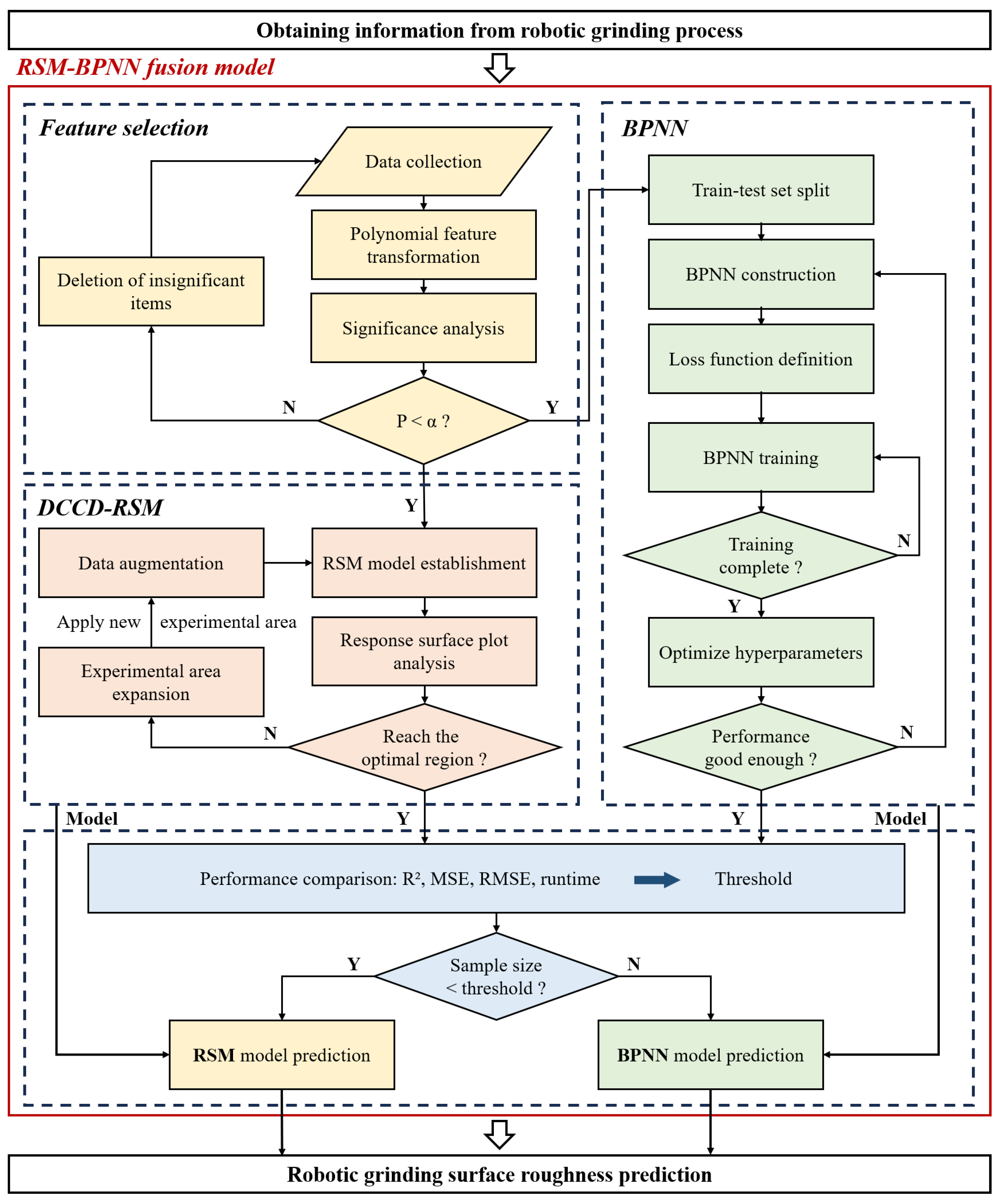
3.1. Overall Framework of BPNN Fusion Model

In this subsection, the BPNN fusion model method is first introduced to provide a predictive model for surface roughness. Then, the BPNN method is broken down into three components—Feature selection, DCCD-RSM model, and BPNN model—followed by a detailed process demonstration and result analysis. This showcases how the entire model framework operates and is applied. The BPNN method is a fusion modeling strategy that combines RSM with BPNN, as illustrated in Figure 2. Initially, the DCCD is employed to select the appropriate experimental region for data collection. The quadratic polynomial regression RSM model is used to fit the relationship between the factors and the response variable. Subsequently, the BPNN module is used to construct the neural network model, which undergoes iterative training and hyperparameter optimization to achieve optimal performance. Finally, the RSM and BPNN models are fused, and the optimal model is selected based on performance metrics comparison. The choice between using the RSM or BPNN for prediction is determined by the input sample size: when the sample size is below a set threshold, the RSM model is preferred; otherwise, the BPNN model is utilized. This method leverages the experimental design advantages of RSM and the robust fitting capabilities of BPNN, enhancing the accuracy and adaptability of parameter optimization and outcome prediction.

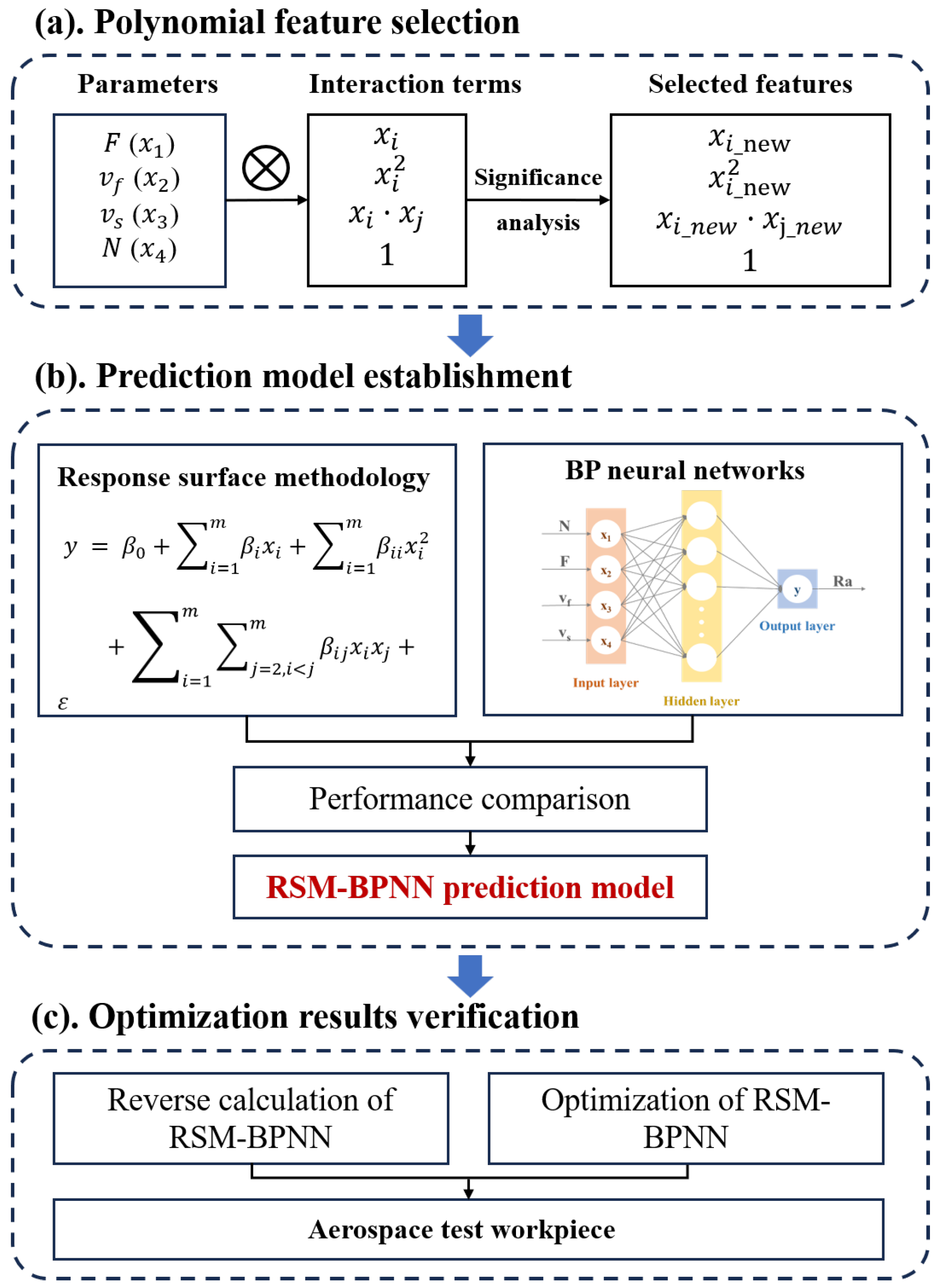
3.1.1. Selection of Polynomial Transformation Feature

In robotic grinding, the workpiece often has specific contour requirements after grinding. The shape of the workpiece is, therefore, a key consideration. Cutting depth, as it can help control the surface contour to some extent, is typically used as one of the input parameters. However, in the robotic grinding scenario discussed in this paper, the target workpieces are irregularly shaped small-batch parts. The goal is not to transform these parts into specific shapes but rather to reduce surface roughness and improve surface quality without significantly altering their original appearance.

Grinding force, as a control parameter, offers greater adaptability and reduces the risk of over-grinding. Through stable force-position hybrid control, the robot’s grinding end-effector maintains constant contact with the workpiece surface, ensuring good surface quality and consistency while preserving the original contour. Furthermore, during the actual grinding process, the grinding force provides a more stable and controllable way to assess the grinding state. By monitoring the grinding force, it is easier to identify issues such as under-grinding or over-grinding, which could lead to surface defects. On the other hand, monitoring cutting depth requires additional measurement tools and technical support. Therefore, in this paper, cutting depth is removed as an input parameter and replaced by grinding force.

Based on the above theory, polynomial features are generated by performing a polynomial transformation on four selected variables. An Analysis of Variance(ANOVA) was performed on the data collected from the preliminary experiment to determine whether the various features significantly affect surface roughness. The F statistic is calculated as:

$$F={\displaystyle \frac{{\mathrm{MS}}_{\mathrm{between}}}{{\mathrm{MS}}_{\mathrm{within}}}}={\displaystyle \frac{\frac{{\mathrm{SS}}_{\mathrm{between}}}{{\mathrm{df}}_{\mathrm{between}}}}{\frac{{\mathrm{SS}}_{\mathrm{within}}}{{\mathrm{df}}_{\mathrm{within}}}}}$$

(1)

where:

• ${\mathrm{MS}}_{\mathrm{between}}$ and ${\mathrm{MS}}_{\mathrm{within}}$ represent the between-group mean square and within-group mean square, respectively,
• ${\mathrm{SS}}_{\mathrm{between}}$ and ${\mathrm{SS}}_{\mathrm{within}}$ represent the sum of squares for between-group and within-group variances, respectively,
• ${\mathrm{df}}_{\mathrm{between}}$ and ${\mathrm{df}}_{\mathrm{within}}$ are the corresponding degrees of freedom.

The F-test is used to compute the p-value:

$$p=P(F>F_{\mathrm{calculated}})$$

(2)

If the p-value is smaller than the predetermined significance level ($\alpha =0.05$), the null hypothesis of “no significant effect” ($H_0$) is rejected. It is concluded that the polynomial features have a significant effect on the outcome.

3.1.2. Design and Establishment of DCCD-RSM

In order to determine the appropriate range of parameters, exploratory experiments were carried out in the early stage. It is observed that the extreme conditions of the grinding parameters can lead to under-grinding or over-grinding of the workpiece surface. Underwear results in incomplete removal of surface materials, while overwear results in workpiece surface defects and damage, ultimately reducing surface roughness. In order to ensure the smoothness and integrity of surface machining, Dynamic Central Composite Design (DCCD) was used to find out the appropriate parameter range.

Initially, a pre-experiment is carried out using the central composite design to collect response data from the region of interest and create a quadratic polynomial model of the response surface. By analyzing the response surface map and contour map, the region with a low response value is identified. The experimental design is modified using the data from the new experimental point, the experimental area is expanded, and the experimental points are dynamically added outside the boundary when the experimental area does not reach the optimal area. This process continues until the ideal experimental location is found.

To model and analyze the relationship between multiple input variables and a response variable, DCCD-RSM is used, and the model equation can be expressed as:

$$y={\beta }_0+\sum _{i=1}^m{\beta }_i{x}_i+\sum _{i=1}^m{\beta }_{ii}{x}_i^2+\sum _{i=1}^m\sum _{j=i+1}^m{\beta }_{ij}{x}_i{x}_j+\epsilon$$

(3)

where y represents the response variable, and $x_i$ and $x_j$ are the values of the i-th and j-th independent variables, respectively. ${\beta }_0$ is the intercept, while ${\beta }_i$, ${\beta }_{ii}$, and ${\beta }_{ij}$ denote the coefficients of the linear, quadratic, and interaction terms, respectively. The error term $\epsilon$ accounts for any unexplained variability in the data, and m represents the number of input variables.

To fit the model, the coefficients ${\beta }_0$, ${\beta }_i$, ${\beta }_{ii}$, and ${\beta }_{ij}$ are estimated using least squares regression by minimizing the residual sum of squares (RSS):

$$\mathrm{RSS}=\sum _{k=1}^n{(y_k-{\widehat{y}}_k)}^2$$

(4)

where n is the number of data points, $y_k$ is the observed value, and ${\widehat{y}}_k$ is the predicted value from the model.

For clarity, the response surface model can also be expressed in matrix form:

$$\widehat{y}=x^{\top }Bx+b^{\top }x+{\beta }_0$$

(5)

where $x=[1,x_1,x_2,\cdots ,x_m]$ is the input variable vector (with a constant term), B is a symmetric matrix containing quadratic and interaction coefficients, and b is a vector of linear coefficients.

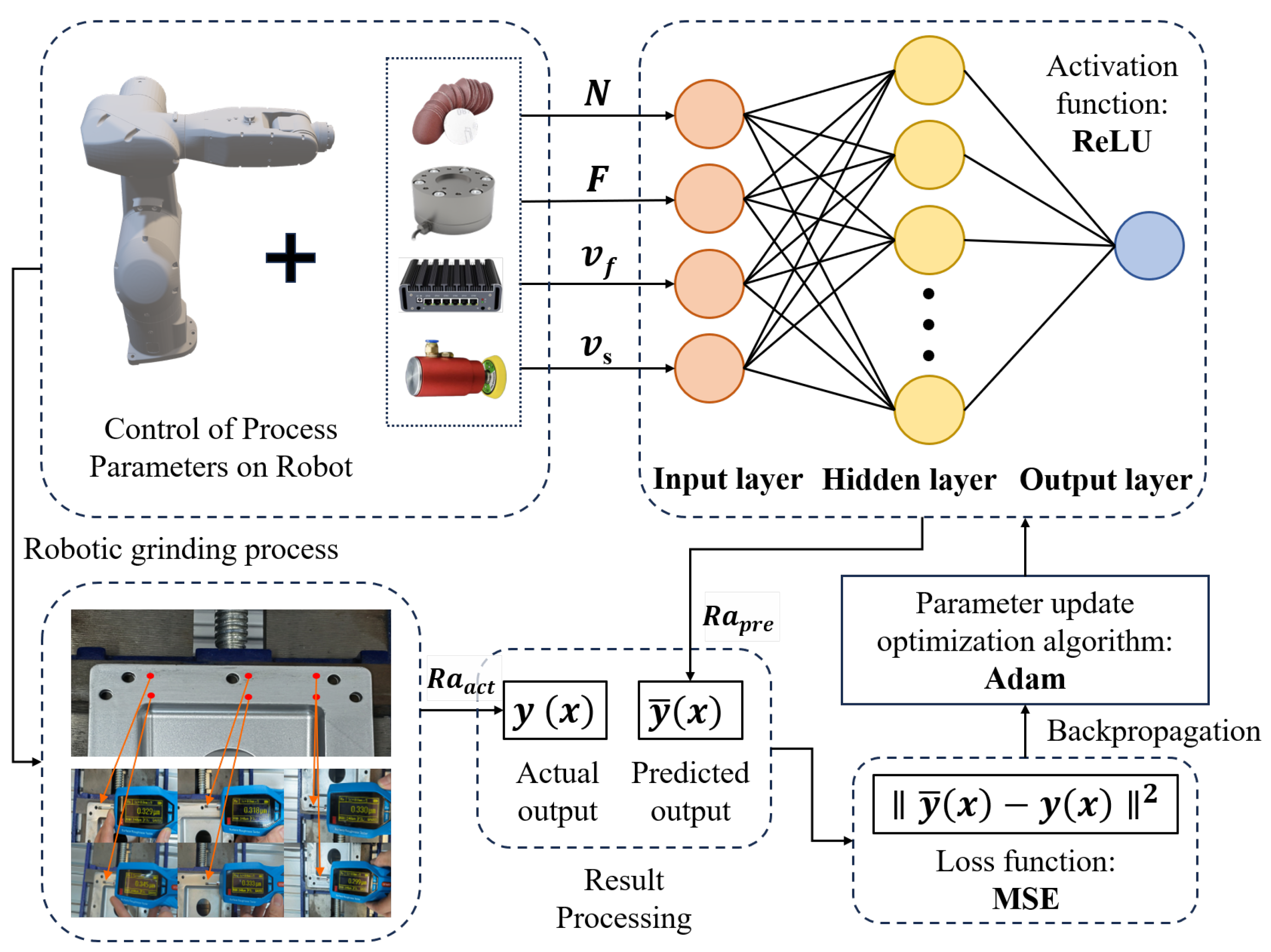
3.1.3. Structure and Training Design of BPNN

To model complex relationships, BPNN consists of input, hidden, and output layers, each containing multiple neurons. The network adjusts connection weights by learning from the training data. Figure 3 illustrates the structure of the neural network.

The goal of minimizing the loss function is achieved through the backpropagation process, which utilizes an optimization algorithm to update the network’s weights and biases. The loss function, defined by the following formula, represents the squared difference between predicted output and actual output, commonly known as MSE. To mitigate the risk of overfitting, an L2 regularization term is added to the loss function. The loss function is finally expressed as:

$$C(w,b)={\displaystyle \frac{1}{2n}}{\sum }_x\left(\parallel \overline{y}{\left(x\right)-y\left(x\right)\parallel }^2\right)+{\displaystyle \frac{\lambda }{2n}}{\sum }_w{w}^2$$

(6)

where $C(w,b)$ represents the loss function, where w and b denote the weights and biases, respectively, n is the number of training samples, ${\sum }_x$ indicates summation over all training samples x, $\overline{y}\left(x\right)$ is the predicted output of the neural network on sample x, $y\left(x\right)$ is the actual output, $\lambda$ is the regularization parameter, and ${\sum }_w$ represents summation over all weights w.

3.2. Robotic Grinding Process Parameters Optimization

The robotic grinding parameters for the grinding process are determined by optimizing the BPNN model. For the RSM part, numerical optimization is used, while for the BPNN part, Genetic Algorithm-Simulated Annealing(GA-SA) optimization is employed.

3.2.1. Robotic Parameters Optimization on RSM

To optimize the response variable y, RSM seeks the optimal combination of input variables by solving the following optimization problem:

$$\mathrm{Find}\{x_1,x_2,\cdots ,x_m\}\mathrm{such}\mathrm{that}max/miny=f(x_1,x_2,\cdots ,x_m)$$

(7)

where y is the response variable and $\{x_1,x_2,\cdots ,x_m\}$ are the input variables. The goal is to adjust the values of the input variables to maximize or minimize the response variable y.

Moreover, to locate the optimal point, the gradient of the response surface is calculated and set to zero:

$${\displaystyle \frac{\partial y}{\partial x_i}}={\beta }_i+2{\beta }_{ii}{x}_i+\sum _{j\ne i}{\beta }_{ij}{x}_j=0,\mathrm{for}i=1,2,\cdots ,m$$

(8)

This equation represents a system of equations for each input variable $x_i$. Solving this system gives the optimal values of the input variables that yield the extreme value of the response variable.

3.2.2. Robotic Parameters Optimization on BPNN

To optimize the response variable y, the GA is used to determine the optimal parameter combinations in the BPNN. However, due to its reliance on random search, it is susceptible to becoming trapped in local optima. To address this issue, SA is incorporated into the GA process (GA-SA), further optimizing individuals with higher fitness, therefore improving overall optimization performance.

The procedure works as follows: first, the Genetic Algorithm runs for 50 generations, generating a set of solutions and selecting individuals based on their fitness. Individuals with higher fitness are chosen as the initial candidates for local search. Then, Simulated Annealing is applied to these individuals to further optimize them and potentially find better local optima. In the SA process, the initial temperature is set high, allowing worse solutions to be accepted, and as the temperature decreases, the algorithm converges toward the optimal solution.

To quantify the fitness of each individual, the objective is to minimize a loss function, such as the MSE:

$$f={\displaystyle \frac{1}{N}}\sum _{i=1}^N{\left(y_i-{\widehat{y}}_i\right)}^2$$

(9)

where f is the fitness value, $y_i$ is the actual output, ${\widehat{y}}_i$ is the predicted output, and N is the number of data points.

Additionally, a regularization term can be added to the objective function to prevent overfitting:

$$C\left(w\right)={\displaystyle \frac{1}{N}}\sum _{i=1}^N{\left(y_i-{\widehat{y}}_i\right)}^2+\alpha {\parallel \mathbf{w}\parallel }^2$$

(10)

where the first term represents the MSE, the second term is the regularization term, ${\parallel \mathbf{w}\parallel }^2$ is the L2 norm of the weight vector, and $\alpha$ is the regularization coefficient.

This hybrid optimization approach combines the global search capability of GA and the local optimization power of SA, enhancing both the precision and efficiency in solving complex optimization problems.

4. Experimental Platform Setup

The industrial robot grinding experimental platform is shown in Figure 4. The setup features an ESTUN robotic arm (Nanjing, China), with a flange at the end-effector to hold a six-axis force sensor and a grinding head for precise material removal. An oil-free, silent air compressor serves as the pneumatic device, and the maximum rotation speed of the grinding head is 9000 rpm. Surface roughness $R_a$ represents the average deviation of the surface profile over a given length. It is used due to its simple calculation and effective reflection of the overall level of surface roughness. The calculation formula is as follows:

$$R_a={\displaystyle \frac{1}{l}}{\int }_0^l\left|y\left(x\right)\right|dx$$

(11)

where $y\left(x\right)$ is the height of the surface profile over a length l.

Surface-roughness data processing is conducted using a Gaussian filter. The evaluation length of the contact surface-roughness instrument is 4 mm (0.8 mm × 5), and the accuracy error of surface roughness is specified as 0.005 $\mathsf{\mu }$m.

5. Results

The experiment results use the BPNN method to model the surface roughness of grinding results based on the selected feature data, including polynomial feature selection, prediction model establishment, and optimization results verification as shown in Figure 5.

5.1. Polynomial Feature Selection

The significance of the 15 polynomial features derived from the grinding force (F), feed rate ($v_f$), wheel speed ($v_s$), and grit size (N) was evaluated and optimized using ANOVA, eliminating features with P values exceeding the significance threshold to refine the data preprocessing. Through this optimization process, the ANOVA results identified $v_s$ as the most significant factor influencing surface roughness, followed by $v_f$. Furthermore, it was found that the square term of $v_f$, the interaction term between F and $v_f$, and the interaction term between F and $v_s$ had no significant impact on the model. By removing these insignificant polynomial features, the model inputs were further optimized to better capture the underlying relationships. The remaining polynomial features after eliminating the insignificant terms are shown in

Table 1. Selected features after selection.

Feature Type	Selected Features
Constant Term	1
Linear Terms	$F,v_f,v_s,N$
Quadratic Terms	$F^2,v_s^2,N^2$
Interaction Terms	$F·N,v_f·v_s,v_f·N,v_s·N$

.

5.2. Prediction Model Establishment

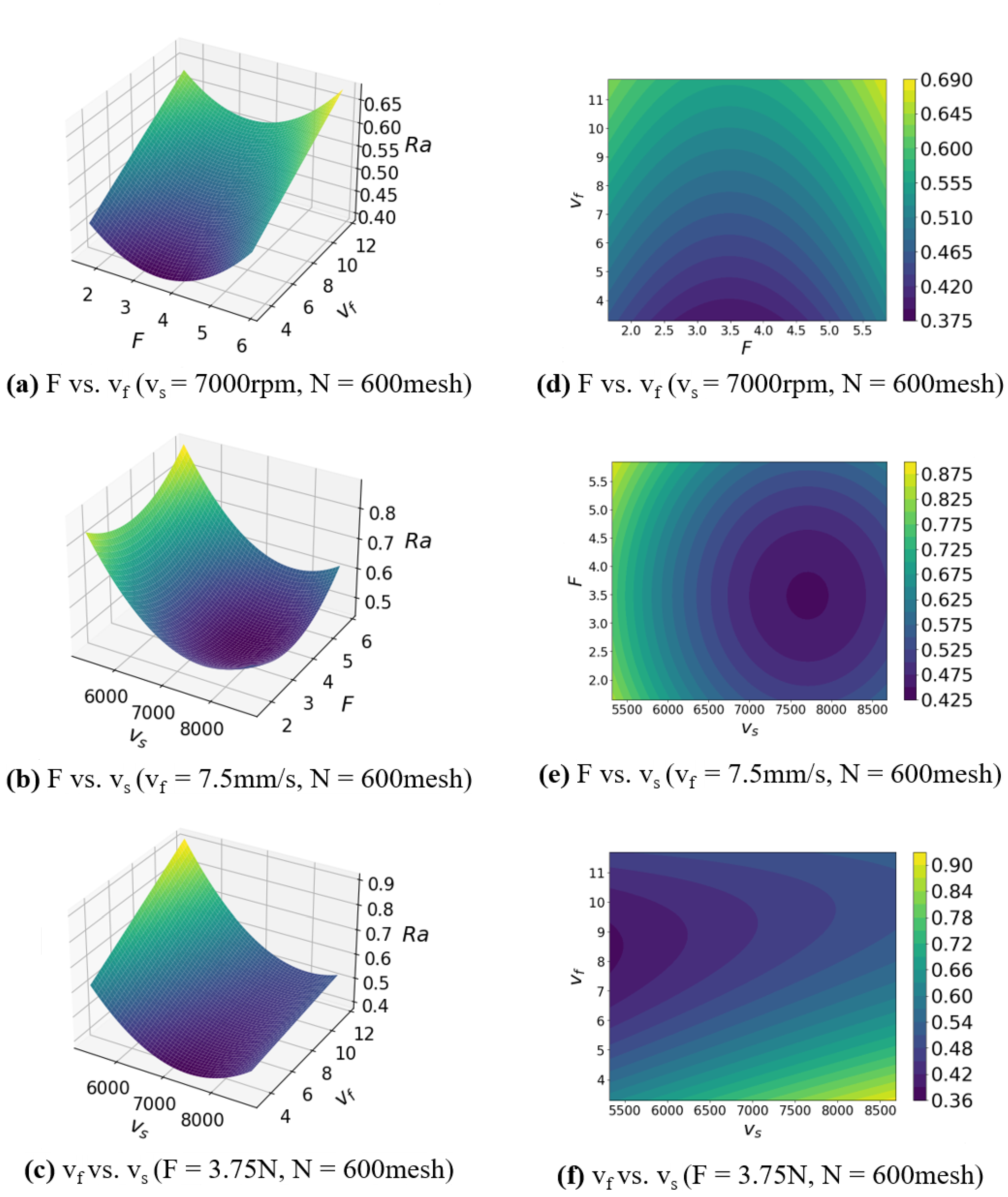
5.2.1. Result and Analysis of DCCD-RSM

DCCD enables rapid identification of the optimal experimental range even without prior experience. The development and application of this method lay the foundation for faster process optimization, conserving resources, and avoiding frequent, time-consuming trial-and-error experiments typically needed to achieve the desired experimental range. This method addresses the practical challenges of selecting experimental ranges in aluminum alloy processing effectively.

Based on the results collected from DCCD, parameter ranges were selected as shown in

Table 2. Parameter symbols and levels of DCCD.

Factor	Coded Symbol	Low Level	High Level
Grinding force (N)	F	2.5	5
Feed rate (mm/s)	$v_f$	5	10
Wheel speed (rpm)	$v_s$	6000	8000
Grit size	N	*	*

“*” means the discrete variable N has no high or low levels here

, and three Discrete N (400, 600, 800) were selected for testing to conduct response analysis and determine the relationship between various factors and surface roughness. Through this designed DCCD-RSM, the model of surface roughness was developed in Equation (12):

$$\begin{array}{cc}\hfill y=& 3.2141-1.8614\times {10}^{-1}F+9.0322\times {10}^{-2}{v}_f-7.7827\times {10}^{-4}{v}_s\hfill \\ \hfill & +7.4796\times {10}^{-4}N+2.1104\times {10}^{-2}{F}^2+2.7717\times {10}^{-5}FN\hfill \\ \hfill & -8.6737\times {10}^{-6}{v}_f{v}_s-1.5783\times {10}^{-5}{v}_{f}N+5.5720\times {10}^{-8}{v}_s^2\hfill \\ \hfill & -2.6393\times {10}^{-8}{v}_{s}N-4.7448\times {10}^{-7}{N}^2\hfill \end{array}$$

(12)

According to the fitting results above, the response surface plots and the contour plots of the grinding process are shown in Figure 6. The strategy used for the remaining two variables is to fix them at their midpoint values. Figure 6a,d depict the response surface and contour plots of F and $v_f$ on surface roughness. Surface roughness increases with increasing $v_f$ and initially decreases with increasing F before increasing again. There is a minimum value of surface roughness when F is around 3.5 N at a given $v_f$. Figure 6b,e illustrate the response surface and contour plots of $v_s$ and F. Surface roughness decreases initially with both $v_s$ and F before increasing again. When F is around 3.5 N, and $v_s$ is approximately 7700 rpm, the surface roughness reaches a minimum. Figure 6c,f present the response surface and contour plots of $v_s$ and $v_f$. Surface roughness increases with increasing $v_f$. When $v_s$ is around 5000 rpm, there is a significant reduction in surface roughness, while the reduction is less pronounced when $v_s$ is around 9000 rpm. A minimum value of surface roughness is observed when $v_s$ is approximately 7400 rpm at a given $v_f$.

5.2.2. Training Process and Results of BPNN

BPNN requires corresponding hyperparameter adjustments based on different data to ensure that the BPNN model achieves optimal performance in the task. Hyperparameter adjustments include but are not limited to learning rate, number of hidden layer nodes, number of iterations, and regularization parameters. By adjusting hyperparameters, the performance of the model is optimized, leading to improved accuracy and generalization ability in the task. To expedite the convergence speed of the model, data preprocessing was performed to normalize it within the range of 0 to 1 and then divided into training, validation, and test sets in a ratio of 7:1.5:1.5.

The final training process of the BPNN is illustrated in Figure 7. The data shown is sampled, with each epoch in the plot being formed every 10 iterations. During the iterations, the best performance of the validation set occurred at the 886th iteration, with a MSE of 0.000793 and an $R^2$ of 87.74%, indicating that the model has converged. In the subsequent models depicted in the MSE and $R^2$ graphs, the three lines representing the training, validation, and test sets exhibit minimal fluctuations during the training process, indicating good convergence stability. This effectively avoids overfitting and underfitting phenomena, resulting in a stable predictive model.

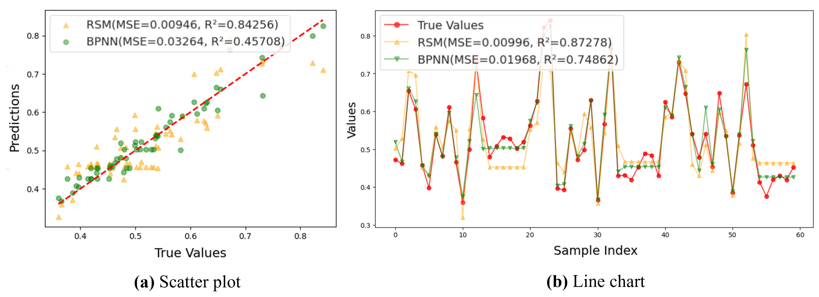
5.2.3. Prediction Comparison Between RSM and BPNN of 60 Sets Data

Through the application of the aforementioned two methods, modeling of the input and output variables of the grinding process was conducted, coupled with regression analysis to evaluate the models. When fitting with 60 sets of real data, the comparison between the predicted values and the actual values on the entire dataset for the two methods is shown in Figure 8a. The prediction of surface roughness using three models and the comparison with the measured values are depicted in Figure 8b. For an experimental dataset of 60 sets, the $R^2$ values for the test set and the entire dataset using the response surface method were 71.26% and 76.46%, respectively. Meanwhile, the $R^2$ values for the test set and the entire dataset using the BPNN method were 83.49% and 93.30%, respectively. These final results indicate that, in this scenario, the BPNN model demonstrates a good fitting effect.

5.3. Optimization Results Verification

5.3.1. Parameters Reverse Calculation and Optimization of BPNN

The verification experiment process is shown in Figure 9. Initially, 20 target surface-roughness values were randomly selected, along with their corresponding experimental sample sizes. The threshold for the experimental sample size was then determined, and a reverse calculation was performed to derive the corresponding robotic grinding parameters. Using these optimized parameter combinations, robotic grinding experiments were conducted on the test workpiece 20 times individually.

In Figure 10, the symbol square represents the random target surface-roughness values, and the symbol triangle represents the true surface-roughness values obtained from grinding experiments using the above parameter combinations. It can be observed that in the random target surface-roughness prediction task using the BPNNprediction model, the MAPE and RMSE between the target values and the actual values is 6.60% and 0.410 $\mathsf{\mu }$m, which demonstrates the accuracy and reliability of the BPNNprediction model.

30 and 60 groups of small-sample data are used as the test sample size. Through threshold detection by RSM-BPN, optimization methods, including RSM-numerical optimization and BPNN-genetic algorithm optimization, are employed. The optimal robotic control parameter combinations are shown in

Table 3. Combinations of predicted and optimized surface-roughness values.

Sample Size	F(N)	${\mathit{v}}_{\mathit{f}}$ (mm/s)	${\mathit{v}}_{\mathit{s}}$ (rpm)	N	${\mathit{R}}_{\mathit{a}}$ ($\mathsf{\mu }$m)
30	4.1474	3.0000	7312.7826	400	0.3472
60	5.4593	3.4935	7122.5485	600	0.3449

.

For the application of robotic grinding, this subsection shows a comparison of the surface-roughness values based on 20 measurements (each value measured three times)under the same robotic path when the optimal grinding parameters are used versus when they are not (when not used, the central experimental point parameters from DCCD are applied). While the optimal robotic control parameter combinations are applied, the average $R_a$ values are 0.3582 $\mathsf{\mu }$m and 0.3558 $\mathsf{\mu }$m for the 30-sample and 60-sample group sizes, respectively. Compared to the average $R_a$ values obtained without using the optimized robotic parameters and the theoretical optimal $R_a$ value, the relative improvement percentages for the 30-sample and 60-sample experimental datasets are 30.91% and 30.69%, respectively. Additionally, the overall APE and RMSE of the actual experimental results compared to the theoretical values after optimization are 3.15% and 0.0288 $\mathsf{\mu }$m, respectively.

5.3.2. Applications and Verification in Robotic Grinding of Aerospace Test Workpiece

The optimization of parameters determines the quality and consistency of the processed workpiece surface. As can be seen from the test workpiece surface in Figure 11, when the optimal robotic grinding parameters are not used, the grinding marks are prominent, and over- and under-grinding occur. In contrast, after adopting the optimal robotic grinding parameters, the surface quality improves significantly, which is reflected in the improvement of surface roughness. Therefore, robotic grinding parameter modeling and optimization are highly effective and practical for the grinding of aerospace workpieces based on small-sample data.

6. Discussions

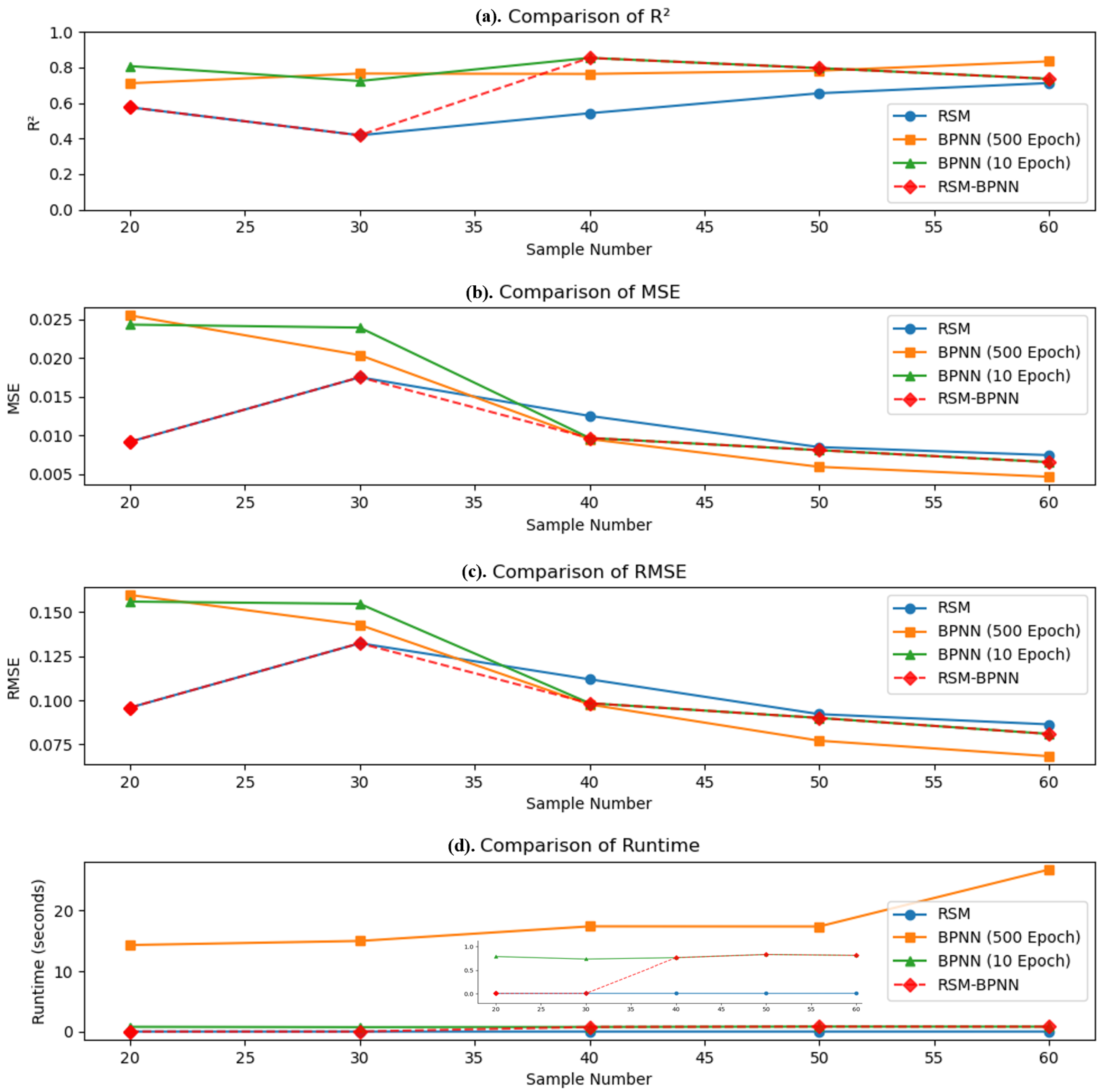
Evaluation Results of BPNN Fusion Method on Variable Small-Sample Data

From an engineering perspective, the tradeoff between accuracy and modeling time must be considered. In order to obtain a modeling method combining RSM and BPNN, the two methods of RSM and BPNN will be compared and analyzed respectively, and the optimal method will be selected under different sample sizes according to specific experimental constraints and requirements to form the BPNN fusion method.

The discussion provides a comparison of the predictive accuracy of the two algorithms based on 60 sets of data. However, in practical usage, the number of data samples often varies significantly due to the scarcity of experimental materials. Therefore, this study designed experiments to measure method selection under different sample sizes. In the following, further investigation will be carried out by conducting training and fitting using 20–60 sets of data for 500 iterations each. The evaluation metrics, including $R^2$, MSE, RMSE, and runtime, will be calculated and analyzed as assessment indicators of the results.

Additionally, from the perspective of transferability in industrial applications, as shown in Figure 12, for both RSM and BPNN with 500 epochs, RSM required significantly less runtime compared to BPNN of the same data size. Since workers are often responsible for repetitive operations and may lack expertise in data processing, RSM can be directly embedded in the teach pendant used by workers as guidance, assisting them in modeling and predicting grinding process parameters. In contrast, BPNN requires preprocessing of data or complex hyperparameter selection, which entails a considerable amount of time for tuning until the model achieves satisfactory performance. Therefore, in terms of usability and transferability, RSM outperforms BPNN with 500 epochs.

To address the issue of the BPNN’s prolonged runtime, a training method of combining 10-iteration BPNN training with RSM is proposed, as indicated by the green line in Figure 12d. It can be clearly observed that, in terms of the $R^2$, BPNN exhibited similar and satisfactory fitting performance for both 500 epochs and 10 epochs. The trends of MSE and RMSE were consistent, and the intersection with RSM also occurred at sample sizes between 30 and 40, indicating that reducing the number of training iterations from 500 epochs to 10 epochs still holds the aforementioned conclusion that the sample size threshold falls between 30 and 40. In terms of runtime, it can be observed that the runtime of BPNN is directly proportional to the number of epochs, with the training duration of 500 epochs being much longer than that of 10 epochs. Comparing the runtime of 10-epoch BPNN with RSM, the runtime of BPNN is still longer than that of RSM, but the individual runtime is consistently less than 1 s, indicating a faster response speed, which meets the requirements of practical industrial applications.

In summary, RSM and 10-epoch BPNN were chosen to compose the proposed BPNN fusion method. Since the sample size threshold obtained in the above experiments is between 30 and 40, we choose to use RSM fitting when it is less than the threshold, and choose 10-epoch BPNN for training when it is greater than the threshold, and finally obtain the BPNN fusion method. As shown in the red line in Figure 12, BPNN avoids the shortcomings of RSM, which is not accurate enough when the data size is large, and BPNN, which has a large overfitting error when the data size is small. By shortening the number of iterations of BPNN, the runtime is reduced to a level suitable for industrial production scenarios. Compared to models using only the RSM or BPNN methods, the proposed model achieved MSE improvements of 62.19%, 26.80%, 22.75%, 4.63%, and 12.11% with sample sizes of 20–60, respectively.

7. Conclusions

This study designs an BPNN model to predict the surface quality of smart manufacturing. The proposed method first normalizes the data and performs polynomial feature transformation. Then, ANOVA is employed to analyze and select significant features. Subsequently, both RSM and BPNN models are used for prediction and evaluation. By reducing the iteration times for training BPNN and evaluating sample sizes, the BPNN model is constructed. Finally, reverse computation and parameter optimization of the established model are performed, and validation experiments on real machines are carried out. The results demonstrate that the proposed BPNN model exhibits excellent predictive performance for the surface roughness of aerospace aluminum alloy workpieces.

The main contributions and conclusions of this study are as follows:

(a)

During the selection of polynomial features after dimensional expansion, ANOVA is adopted to evaluate the significance of process features. Features with p-values exceeding the significance threshold are eliminated, resulting in polynomial interaction features based on four experimental process parameters: grinding force, feed speed, wheel speed, and sandpaper grit size.

(b)

Based on the RSM and BPNN prediction models, an BPNN fusion model is designed. This model combines the reliability of RSM for small sample sizes and the accuracy of BPNN for large sample sizes under varying sample sizes. Taking into account the training time and fitting efficiency, this model is better suited to handle data modeling for single-piece and small-batch workpieces under varying experimental conditions, meeting industrial requirements for efficient model establishment.

(c)

After performing reverse computation and parameter optimization on the model, the optimized parameters are used to calculate the selected feature results for real-machine validation. The experiments validate the applicability of this method in predicting the surface roughness of single-piece and small-batch workpieces in industrial robotic grinding applications.

However, the exploration and application of algorithms in this study are relatively straightforward, leaving room for improvement in the use of more advanced algorithms. Future research could introduce more sophisticated machine learning algorithms and compare their effectiveness.

Future studies may also expand the inputs and outputs of the model. For instance, grinding depth could be added as an input variable, while material removal rate and robotic processing time could be considered to be output variables to construct a multi-objective optimization model, thereby addressing the diverse requirements of different industrial applications. Additionally, future research should consider training and validating the model with larger datasets, incorporating data augmentation or transfer learning for small-sample training to enhance the robustness and generalizability of the model.

References

1. Li, S.; Yue, X.; Li, Q.; Peng, H.; Dong, B.; Liu, T.; Yang, H.; Fan, J.; Shu, S.; Qiu, F. Development and applications of aluminum alloys for aerospace industry. J. Mater. Res. Technol. 2023, 27, 944–983. [Google Scholar] [CrossRef]
2. Pimenov, D.Y.; Kiran, M.; Khanna, N.; Pintaude, G.; Vasco, M.C.; da Silva, L.R.R.; Giasin, K. Review of improvement of machinability and surface integrity in machining on aluminum alloys. Int. J. Adv. Manuf. Technol. 2023, 129, 4743–4779. [Google Scholar] [CrossRef]
3. Li, H.; Zou, L.; Wang, W.; Li, M. Investigation of Undeformed Chip Thickness Model and Surface Roughness Prediction in Belt Grinding. In Proceedings of the ASME 2022 International Mechanical Engineering Congress and Exposition, Columbus, OH, USA, 30 October–3 November 2022; American Society of Mechanical Engineers: New York, NY, USA, 2022; Volume 86632, p. V02AT02A040. [Google Scholar]
4. Xie, Y.; Chang, G.; Yang, J.; Zhao, M.; Li, J. Process optimization of robotic polishing for mold steel based on response surface method. Machines 2022, 10, 283. [Google Scholar] [CrossRef]
5. Yin, F.; Ji, Q.; Cun, C. Data-driven modeling and prediction analysis for surface roughness of special-shaped stone by robotic grinding. IEEE Access 2022, 10, 67615–67629. [Google Scholar] [CrossRef]
6. Li, R.; Wang, Z.; Yan, J. Multi-Objective Optimization of the Process Parameters of a Grinding Robot Using LSTM-MLP-NSGAII. Machines 2023, 11, 882. [Google Scholar] [CrossRef]
7. Tao, F.; Qi, Q.; Liu, A.; Kusiak, A. Data-driven smart manufacturing. J. Manuf. Syst. 2018, 48, 157–169. [Google Scholar] [CrossRef]
8. You Li, S.L.; Yang, L. Experimental study of wet and dry milling effect on surface roughness of TC4 titanium alloy. Mach. Sci. Technol. 2024, 28, 984–1005. [Google Scholar] [CrossRef]
9. Zhu, C.; Gu, P.; Wu, Y.; Liu, D.; Wang, X. Surface roughness prediction model of SiCp/Al composite in grinding. Int. J. Mech. Sci. 2019, 155, 98–109. [Google Scholar] [CrossRef]
10. Umamaheswara Raju, R.; Ravi Kumar, K.; Vargish, K.; Bharath Kumar, M. Machine learning based surface roughness assessment via CNC spindle bearing vibration. Int. J. Interact. Des. Manuf. 2025, 19, 477–494. [Google Scholar] [CrossRef]
11. Pandremenos, J.; Doukas, C.; Stavropoulos, P.; Chryssolouris, G. Machining with robots: A critical review. In Proceedings of the DET2011, 7th International Conference on Digital Enterprise Technology, Athens, Greece, 28–30 September 2011; pp. 1–9. [Google Scholar]
12. Zhu, D.; Feng, X.; Xu, X.; Yang, Z.; Li, W.; Yan, S.; Ding, H. Robotic grinding of complex components: A step towards efficient and intelligent machining–challenges, solutions, and applications. Robot. Comput.-Integr. Manuf. 2020, 65, 101908. [Google Scholar] [CrossRef]
13. Ke, X.; Yu, Y.; Li, K.; Wang, T.; Zhong, B.; Wang, Z.; Kong, L.; Guo, J.; Huang, L.; Idir, M. Review on robot-assisted polishing: Status and future trends. Robot. Comput.-Integr. Manuf. 2023, 80, 102482. [Google Scholar] [CrossRef]
14. Pervez, M.R.; Ahamed, M.H.; Ahmed, M.A.; Takrim, S.M.; Dario, P. Autonomous grinding algorithms with future prospect towards SMART manufacturing: A comparative survey. J. Manuf. Syst. 2022, 62, 164–185. [Google Scholar] [CrossRef]
15. Xiao, Q.; Gao, M.; Chen, L.; Goh, M. Multi-variety and small-batch production quality forecasting by novel data-driven grey Weibull model. Eng. Appl. Artif. Intell. 2023, 125, 106725. [Google Scholar] [CrossRef]
16. Lestari, W.D.; Adyono, N.; Faizin, A.K.; Haqiyah, A.; Sanjaya, K.H.; Nugroho, A.; Kusmasari, W.; Ammarullah, M.I. Optimization of the cutting process on machining time of ankle foot as transtibial prosthesis components using response surface methodology. Results Eng. 2024, 21, 101736. [Google Scholar] [CrossRef]
17. Khalilpourazari, S.; Khalilpourazary, S. Optimization of time, cost and surface roughness in grinding process using a robust multi-objective dragonfly algorithm. Neural Comput. Appl. 2020, 32, 3987–3998. [Google Scholar] [CrossRef]
18. Yang, J.; Zhang, Y.; Huang, Y.; Lv, J.; Wang, K. Multi-objective optimization of milling process: Exploring trade-off among energy consumption, time consumption and surface roughness. Int. J. Comput. Integr. Manuf. 2023, 36, 219–238. [Google Scholar] [CrossRef]
19. Chen, C.C.; Liu, N.M.; Chiang, K.T.; Chen, H.L. Experimental investigation of tool vibration and surface roughness in the precision end-milling process using the singular spectrum analysis. Int. J. Adv. Manuf. Technol. 2012, 63, 797–815. [Google Scholar] [CrossRef]
20. Li, L.; Haghighi, A.; Yang, Y. A novel 6-axis hybrid additive-subtractive manufacturing process: Design and case studies. J. Manuf. Process. 2018, 33, 150–160. [Google Scholar] [CrossRef]
21. Fry, N.R.; Richardson, R.C.; Boyle, J.H. Robotic additive manufacturing system for dynamic build orientations. Rapid Prototyp. J. 2020, 26, 659–667. [Google Scholar] [CrossRef]
22. Wu, X.; Su, C.; Zhang, K. 316L Stainless Steel Thin-Walled Parts Hybrid-Layered Manufacturing Process Study. Materials 2023, 16, 6518. [Google Scholar] [CrossRef]
23. Sahoo, S.; Lo, C.Y. Smart manufacturing powered by recent technological advancements: A review. J. Manuf. Syst. 2022, 64, 236–250. [Google Scholar] [CrossRef]
24. Ozay, C.; Ballikaya, H.; Savas, V. Application of the Taguchi method to select the optimum cutting parameters for tangential cylindrical grinding of AISI D3 tool steel. Mater. Tehnol. 2016, 50, 81–87. [Google Scholar] [CrossRef]
25. Fan, M.; Zhou, X.; Chen, S.; Jiang, S.; Song, J. Study of the surface roughness and optimization of machining parameters during laser-assisted fast tool servo machining of glass-ceramic. Surf. Topogr. Metrol. Prop. 2023, 11, 025017. [Google Scholar] [CrossRef]
26. Krajnik, P.; Kopac, J.; Sluga, A. Design of grinding factors based on response surface methodology. J. Mater. Process. Technol. 2005, 162, 629–636. [Google Scholar] [CrossRef]
27. Zhujani, F.; Abdullahu, F.; Todorov, G.; Kamberov, K. Optimization of Multiple Performance Characteristics for CNC Turning of Inconel 718 Using Taguchi—Grey Relational Approach and Analysis of Variance. Metals 2024, 14, 186. [Google Scholar] [CrossRef]
28. Kahraman, M.F.; Öztürk, S. Experimental study of newly structural design grinding wheel considering response surface optimization and Monte Carlo simulation. Measurement 2019, 147, 106825. [Google Scholar] [CrossRef]
29. Heininen, A.; Santa-aho, S.; Röttger, J.; Julkunen, P.; Koskinen, K.T. Grinding optimization using nondestructive testing (NDT) and empirical models. Mach. Sci. Technol. 2024, 28, 98–118. [Google Scholar] [CrossRef]
30. Nguyen, V.H.; Le, T.T. Predicting surface roughness in machining aluminum alloys taking into account material properties. Int. J. Comput. Integr. Manuf. 2024, 0, 1–22. [Google Scholar] [CrossRef]
31. Kim, G.; Park, S.; Choi, J.G.; Yang, S.M.; Park, H.W.; Lim, S. Developing a data-driven system for grinding process parameter optimization using machine learning and metaheuristic algorithms. CIRP J. Manuf. Sci. Technol. 2024, 51, 20–35. [Google Scholar] [CrossRef]
32. Nguyen, V.-H.; Le, T.-T.; Le, M.V.; Minh, H.D.; Nguyen, A.T. Multi-objective optimization based on machine learning and non-dominated sorting genetic algorithm for surface roughness and tool wear in Ti6Al4V turning. Mach. Sci. Technol. 2023, 27, 380–421. [Google Scholar] [CrossRef]
33. Shao, H.; Xia, M.; Wan, J.; de Silva, C.W. Modified stacked autoencoder using adaptive Morlet wavelet for intelligent fault diagnosis of rotating machinery. IEEE/ASME Trans. Mechatronics 2021, 27, 24–33. [Google Scholar] [CrossRef]
34. Lai, J.Y.; Lin, P.C. Grinded surface roughness prediction using data-driven models with contact force information. In Proceedings of the 2022 IEEE/ASME International Conference on Advanced Intelligent Mechatronics (AIM), Sapporo, Japan, 11–15 July 2022; IEEE: Piscataway, NJ, USA, 2022; pp. 983–989. [Google Scholar]
Figure 1. Overall DMV architecture of the proposed surface quality prediction method.
Applsci 15 01349 g001
Figure 2. The framework of BPNN fusion method in surface-roughness prediction.
Applsci 15 01349 g002
Figure 3. BPNN construction method and backpropagation parameter optimization process.
Applsci 15 01349 g003
Figure 4. Industrial robot grinding workstation system, (a). Industrial robot, (b). End-effector, (c). Experimental platform, (d). Six-dimensional force sensor, (e). Sander, (f). Grinding head, (g). Workpiece.
Applsci 15 01349 g004
Figure 5. Flow chart of experimental operation process in robot grinding.
Applsci 15 01349 g005
Figure 6. Response surface plots and contour map plots of surface roughness for combinations of three consecutive variables.
Applsci 15 01349 g006
Figure 7. Model MSE and R² on the training set, verification set, and test set during the training of BPNN.
Applsci 15 01349 g007
Figure 8. (a). Scatter plot and (b). line chart of RSM and BPNN model with predictive and true values.
Applsci 15 01349 g008
Figure 9. Reverse calculation verification experiment of BPNNon the test workpiece.
Applsci 15 01349 g009
Figure 10. Comparison between target and actual surface roughness on test workpiece.
Applsci 15 01349 g010
Figure 11. Comparison of grinding effects on workpieces under optimal and non-optimal robotic grinding parameters.
Applsci 15 01349 g011
Figure 12. (a). R2, (b). MSE, (c). RMSE and (d). runtime comparison vs. sample size.
Applsci 15 01349 g012