
Deep Autoencoder Framework for Classifying Damage Mechanisms in Repaired CFRP


Abstract
1. Introduction
2. Materials and Methods
2.1. Materials
2.1.1. Material Properties
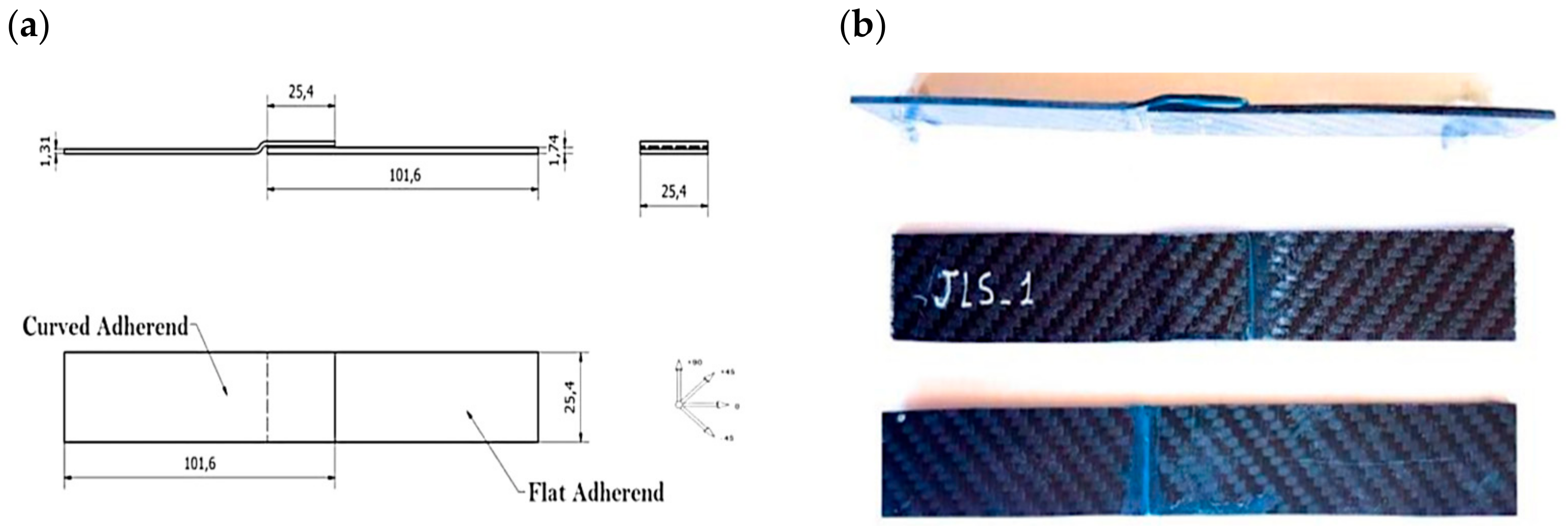
2.1.2. Preparation Methods
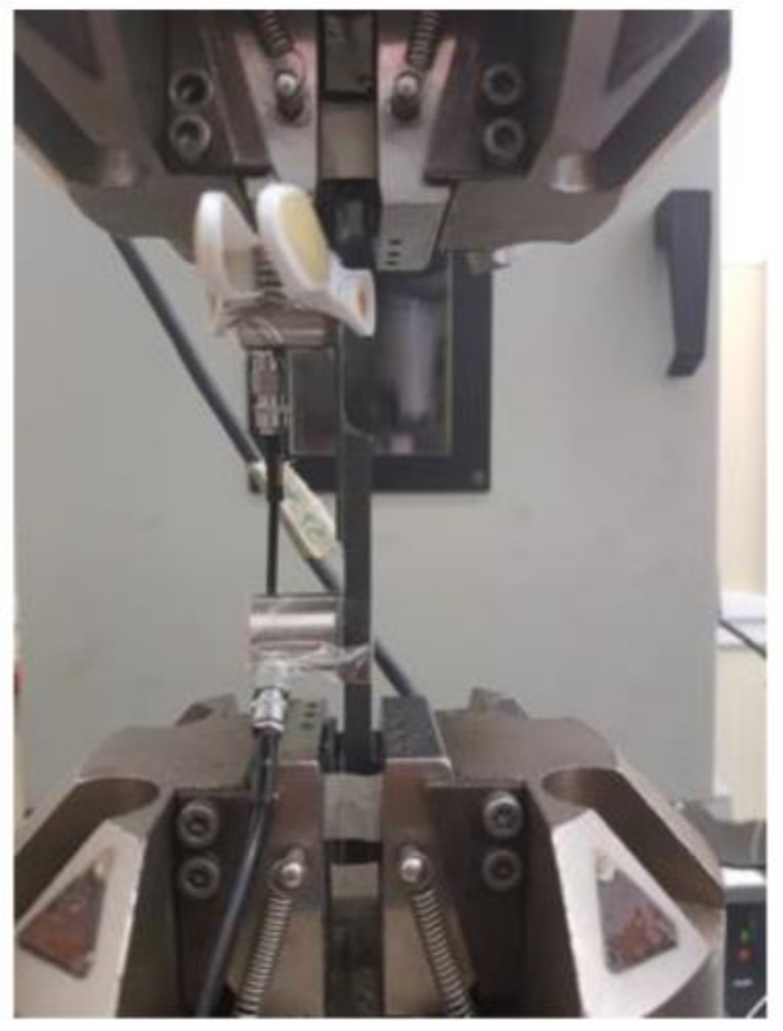
2.1.3. Experimental Procedures
2.2. Methods
2.2.1. Overall Framework
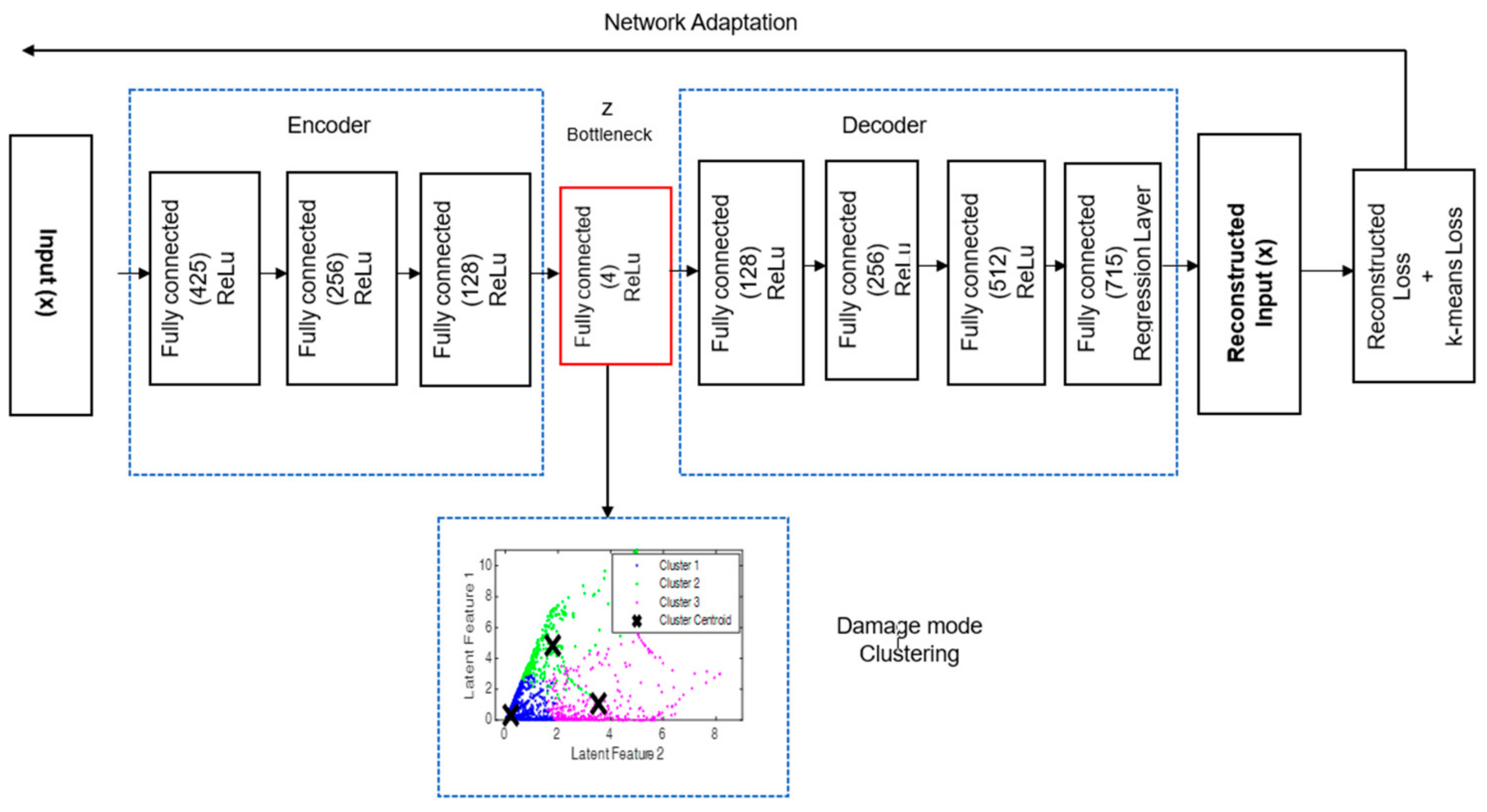
2.2.2. Deep Autoencoder (DAE)
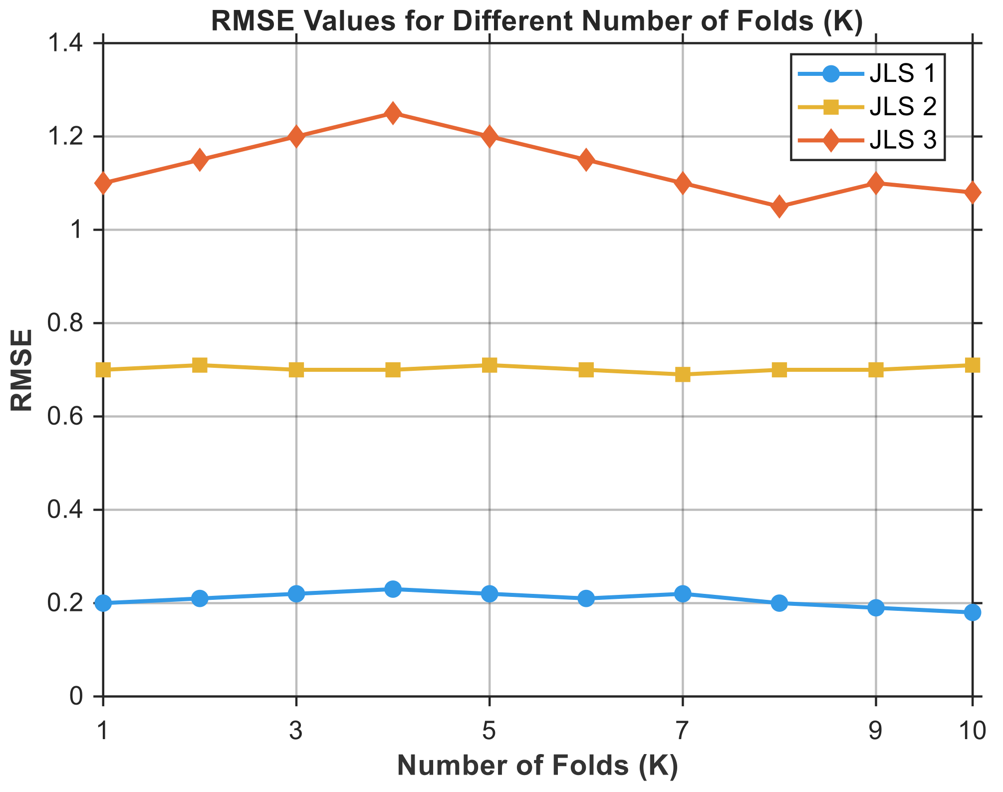
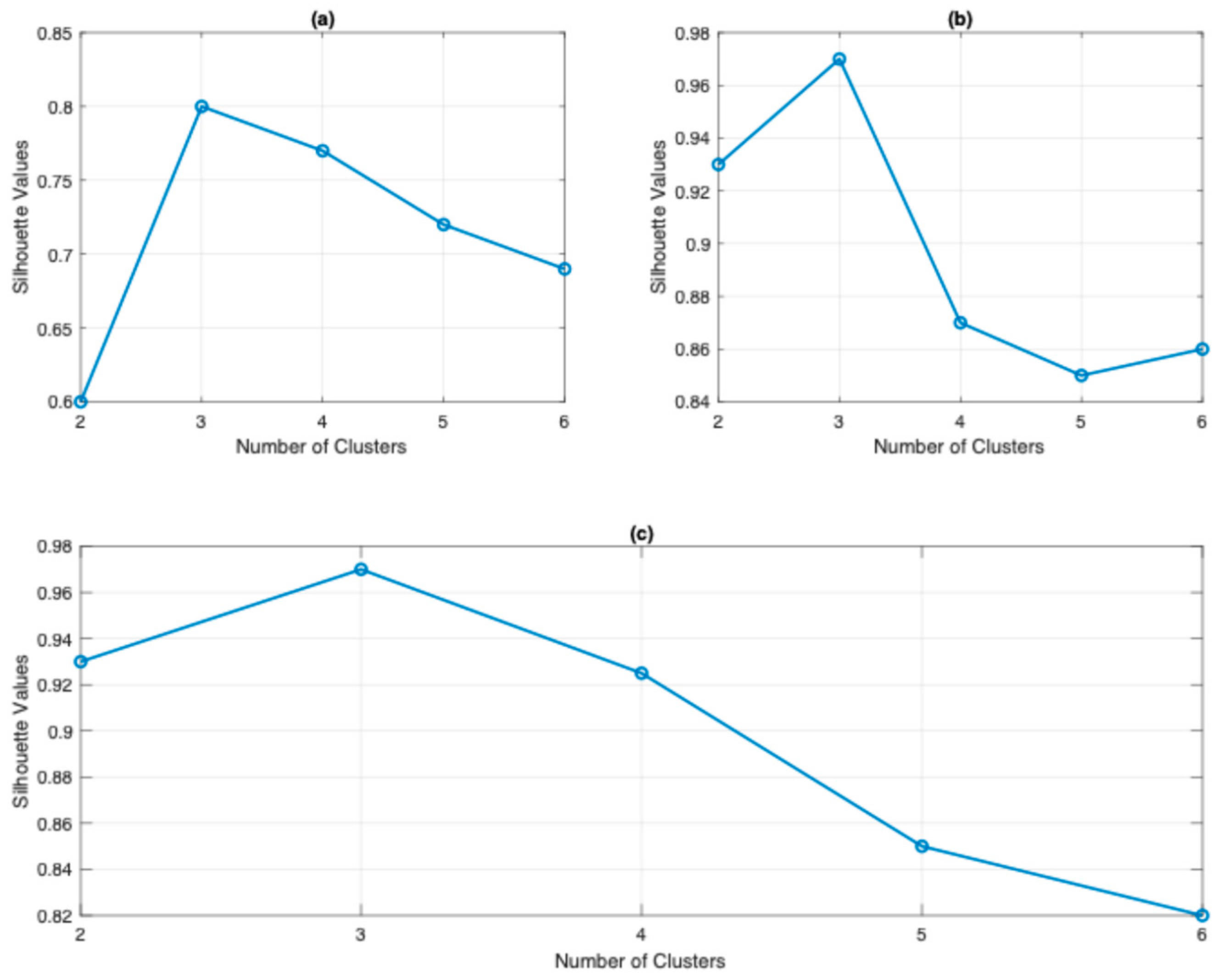
2.2.3. Latent Feature Clustering Using K-Means
3. Results and Discussions
3.1. Mechanical Test Results
3.2. Results of Deep Autoencoder Training
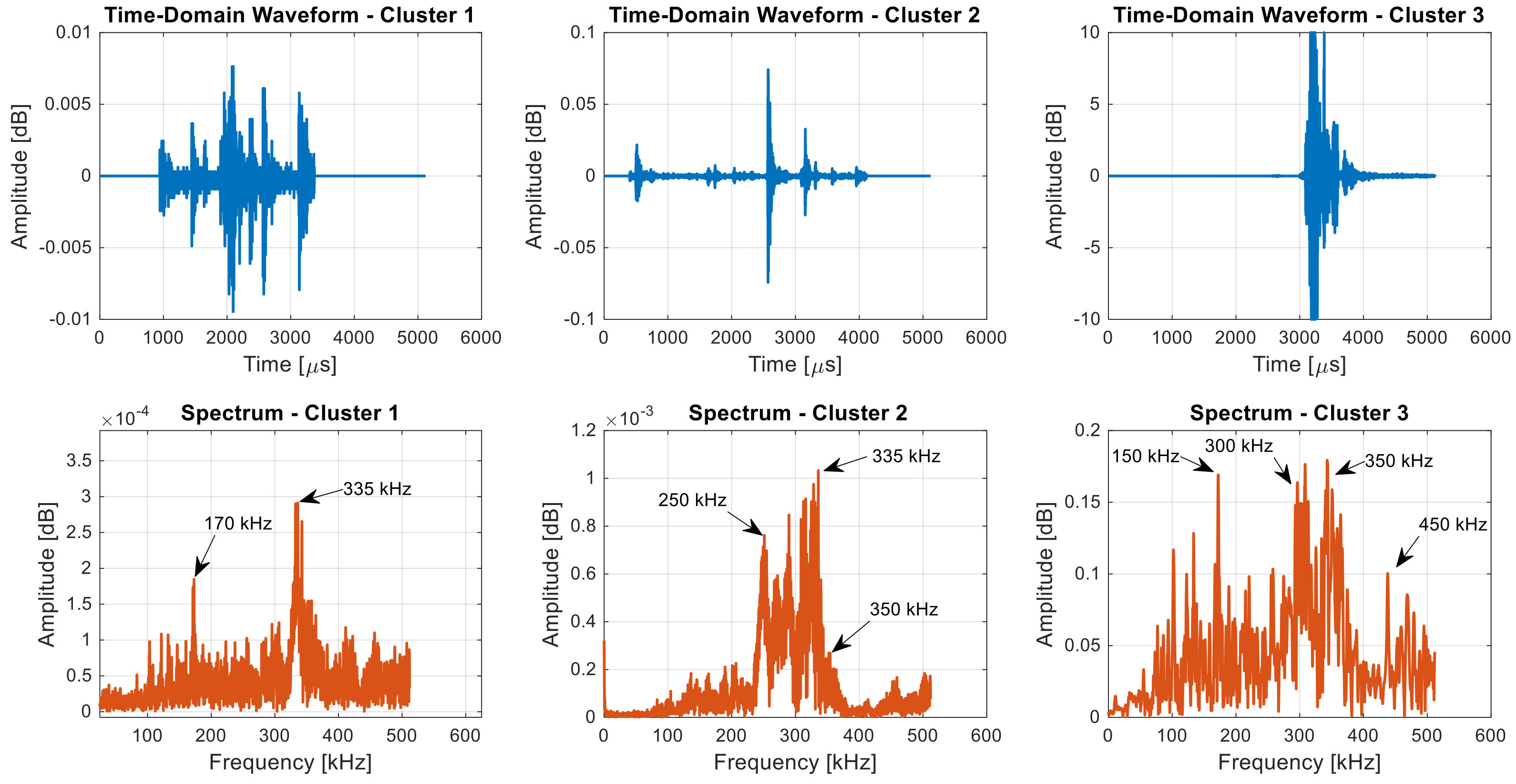
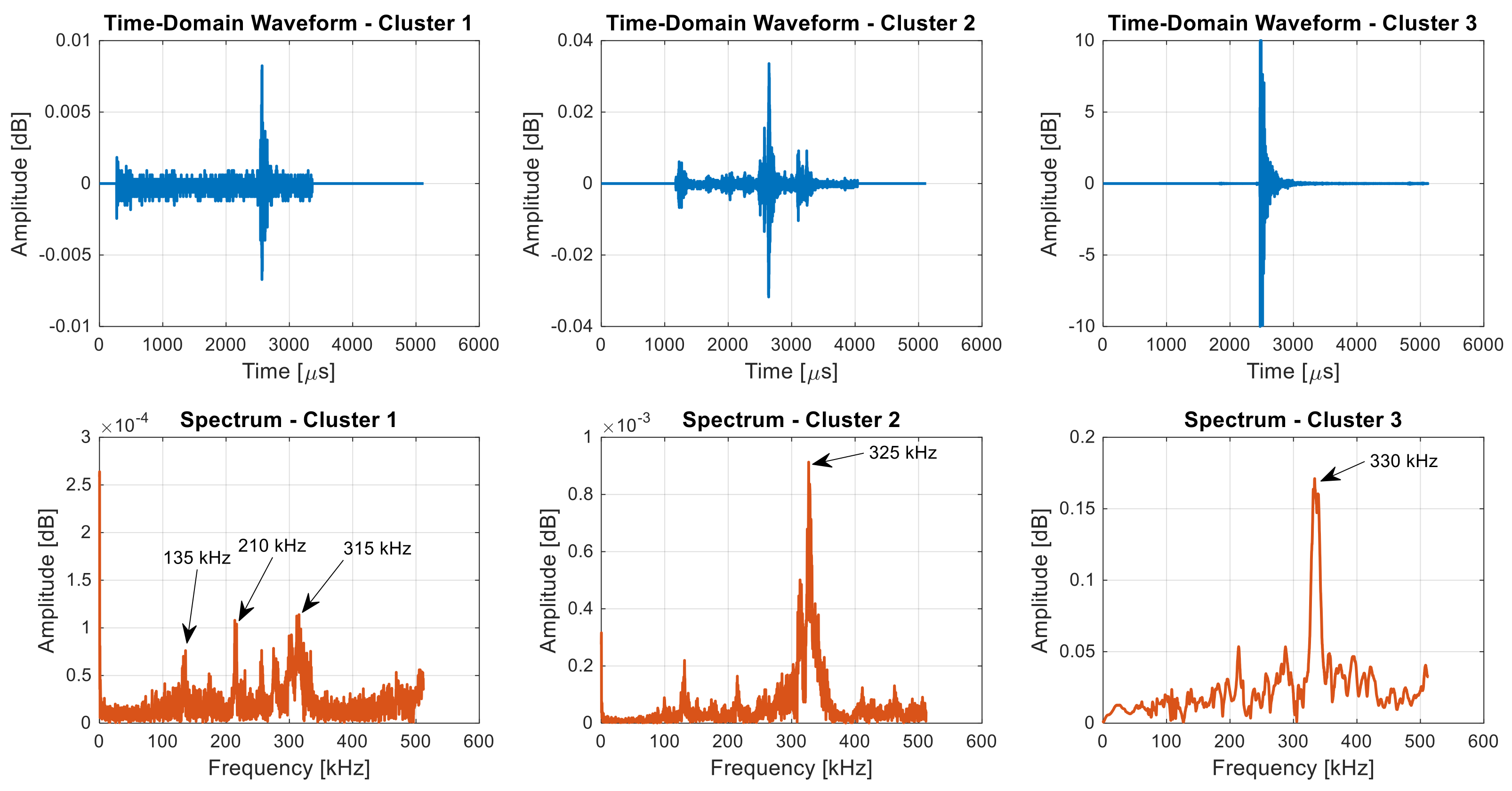
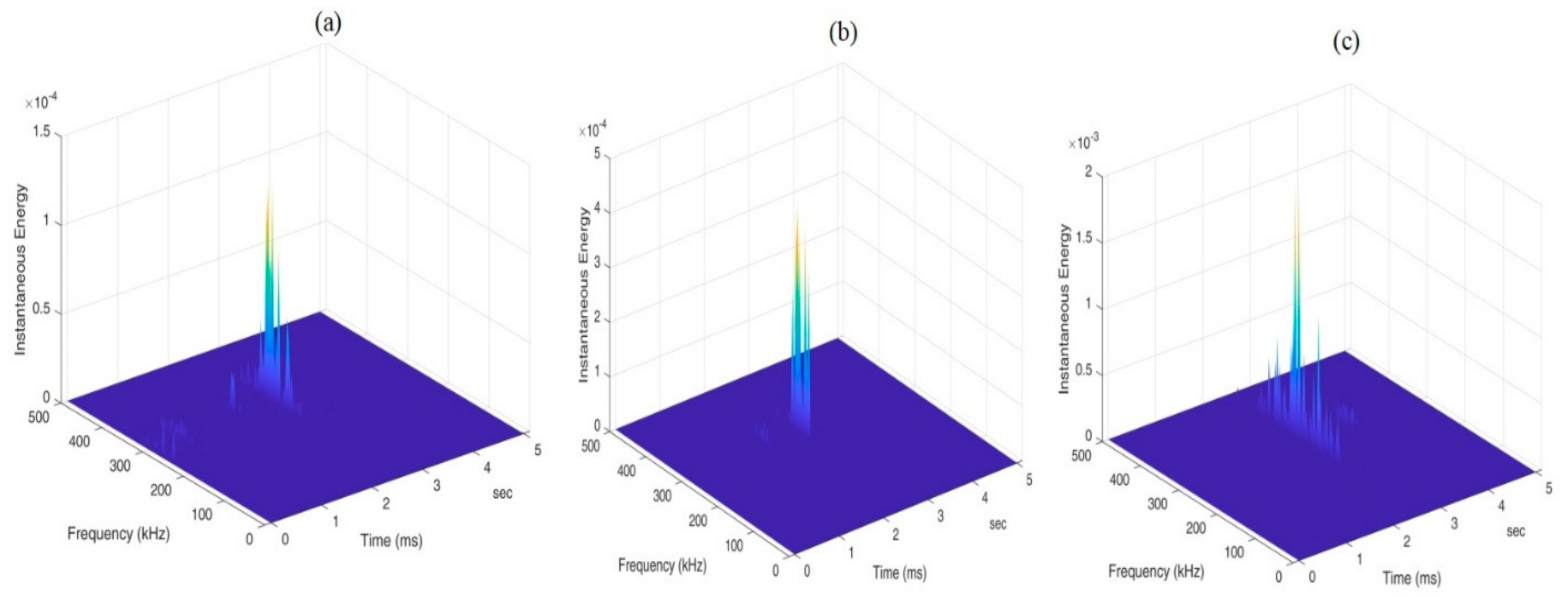
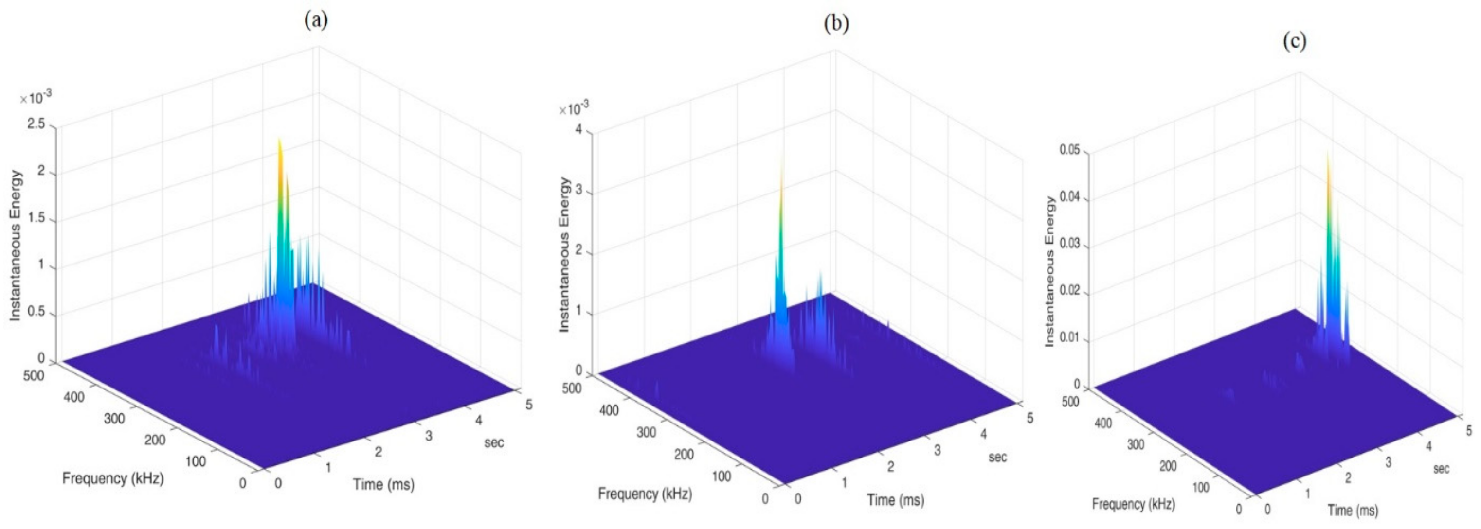
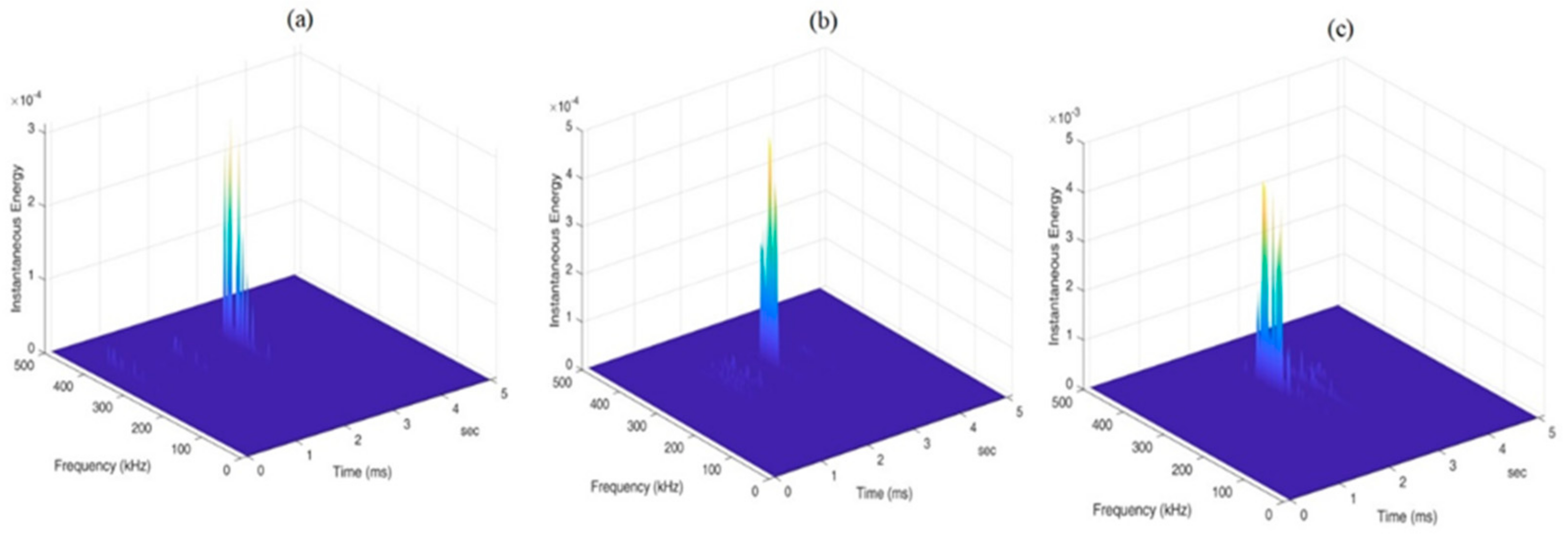
3.3. Damage Characterization Using AE Feature
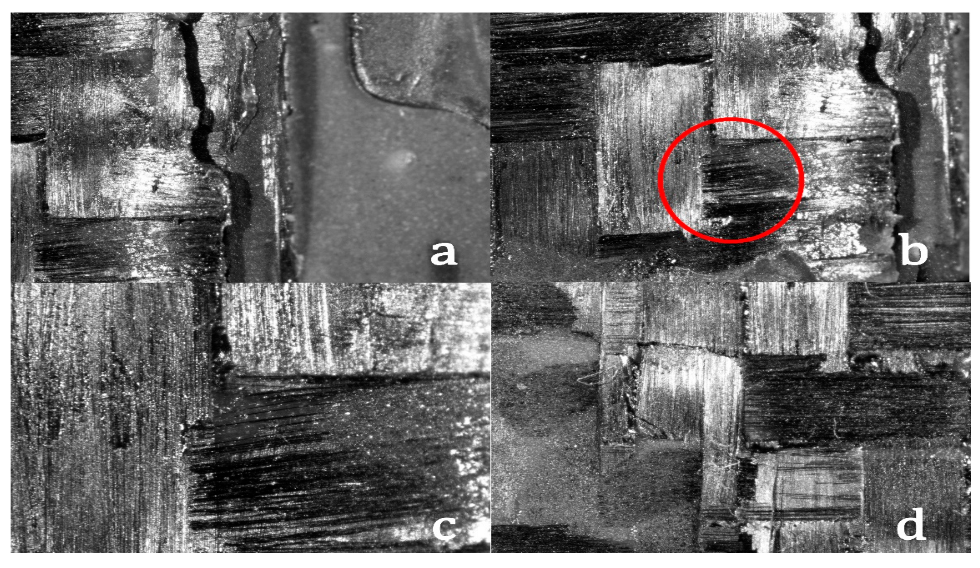
3.4. Fractographic Analysis
4. Conclusions
Author Contributions
Funding
Data Availability Statement
Conflicts of Interest
References
- Chou, C.W.; Liao, W.C.; Wu, S.; Wee, H.M. The Role of Technical Innovation and Sustainability on Energy Consumption: A Case Study on the Taiwanese Automobile Industry. Energies 2015, 8, 6627–6640. [Google Scholar] [CrossRef]
- Jobson, E. Future Challenges in Automotive Emission Control. Top. Catal. 2004, 28, 191–199. [Google Scholar] [CrossRef]
- Mayyas, A.T.; Mayyas, A.R.; Omar, M. Sustainable Lightweight Vehicle Design: A Case Study in Eco-Material Selection for Body-in-White. In Lightweight Composite Structures in Transport: Design, Manufacturing, Analysis and Performance; Woodhead Publishing: Sawston, UK, 2016; pp. 267–302. [Google Scholar] [CrossRef]
- Zhang, W.; Xu, J. Advanced Lightweight Materials for Automobiles: A Review. Mater. Des. 2022, 221, 110994. [Google Scholar] [CrossRef]
- Ahmad, H.; Markina, A.A.; Porotnikov, M.V.; Ahmad, F. A Review of Carbon Fiber Materials in Automotive Industry. IOP Conf. Ser. Mater. Sci. Eng. 2020, 971, 032011. [Google Scholar] [CrossRef]
- Alaneme, K.K.; Fajemisin, A.V.; Maledi, N.B. Development of Aluminium-Based Composites Reinforced with Steel and Graphite Particles: Structural, Mechanical and Wear Characterization. J. Mater. Res. Technol. 2019, 8, 670–682. [Google Scholar] [CrossRef]
- Liu, X.; Tian, S.; Tao, F.; Yu, W. A Review of Artificial Neural Networks in the Constitutive Modeling of Composite Materials. Compos. B Eng. 2021, 224, 109152. [Google Scholar] [CrossRef]
- Sugita, Y.; Winkelmann, C.; La Saponara, V. Environmental and Chemical Degradation of Carbon/Epoxy Lap Joints for Aerospace Applications, and Effects on Their Mechanical Performance. Compos. Sci. Technol. 2010, 70, 829–839. [Google Scholar] [CrossRef]
- Ballo, F.M.; Gobbi, M.; Mastinu, G.; Previati, G. Structural Optimisation in Road Vehicle Components Design. Optim. Lightweight Constr. Princ. 2021, 233–270. [Google Scholar] [CrossRef]
- Romero, C.A.; Correa, A.; Echeverri, E.A.; Vergara, D.; Romero, C.A.; Correa, P.; Anderson, E.; Echeverri, A.; Vergara, D. Strategies for Reducing Automobile Fuel Consumption. Appl. Sci. 2024, 14, 910. [Google Scholar] [CrossRef]
- Kim, K.Y.; Sim, J.; Jannat, N.E.; Ahmed, F.; Ameri, S. Challenges in Riveting Quality Prediction: A Literature Survey. Procedia Manuf. 2019, 38, 1143–1150. [Google Scholar] [CrossRef]
- Yu, Q.Q.; Gao, R.X.; Gu, X.L.; Zhao, X.L.; Chen, T. Bond Behavior of CFRP-Steel Double-Lap Joints Exposed to Marine Atmosphere and Fatigue Loading. Eng. Struct. 2018, 175, 76–85. [Google Scholar] [CrossRef]
- De Araujo, R.; Lima, A.; Bernasconi, A.; Carboni, M. Acoustic Emission Applied to Mode I Fatigue Damage Monitoring of Adhesively Bonded Joints. e-J. Nondestruct. Test. 2023, 28, 1–9. [Google Scholar] [CrossRef]
- Dilger, K. Selecting the Right Joint Design and Fabrication Techniques. In Advances in Structural Adhesive Bonding; Elsevier: Amsterdam, The Netherlands, 2010; pp. 295–315. [Google Scholar] [CrossRef]
- Mallick, P.K. Joining for Lightweight Vehicles. In Materials, Design and Manufacturing for Lightweight Vehicles; Elsevier: Amsterdam, The Netherlands, 2010; pp. 275–308. [Google Scholar] [CrossRef]
- Burt, V. Adhesive Bonding. In Aluminum Science and Technology; Springer Science\& Business Media: Berlin/Heidelberg, Germany, 2018; pp. 783–789. [Google Scholar] [CrossRef]
- Liu, Y.; Carnegie, C.; Ascroft, H.; Li, W.; Han, X.; Guo, H.; Hughes, D.J. Investigation of Adhesive Joining Strategies for the Application of a Multi-Material Light Rail Vehicle. Materials 2021, 14, 6991. [Google Scholar] [CrossRef] [PubMed]
- Li, G.; Pang, S.S.; Woldesenbet, E.; Stubblefield, M.A.; Mensah, P.F.; Ibekwe, S.I. Investigation of Prepreg Bonded Composite Single Lap Joint. Compos. B Eng. 2001, 32, 651–658. [Google Scholar] [CrossRef]
- Zhao, W.; Pei, N.; Xu, C. Experimental Study of Carbon/Glass Fiber-Reinforced Hybrid Laminate Composites with Torsional Loads by Using Acoustic Emission and Micro-CT. Compos. Struct. 2022, 290, 115541. [Google Scholar] [CrossRef]
- Taib, A.A.; Boukhili, R.; Achiou, S.; Boukehili, H. Bonded Joints with Composite Adherends. Part II. Finite element analysis of joggle lap joints. Int. J. Adhes. Adhes. 2006, 26, 237–248. [Google Scholar] [CrossRef]
- Gresil, M.; Revol, V.; Kitsianos, K.; Kanderakis, G.; Koulalis, I.; Sauer, M.O.; Trétout, H.; Madrigal, A.M. EVITA Project: Comparison Between Traditional Non-Destructive Techniques and Phase Contrast X-Ray Imaging Applied to Aerospace Carbon Fibre Reinforced Polymer. Appl. Compos. Mater. 2017, 24, 513–524. [Google Scholar] [CrossRef]
- Cawley, P. The Rapid Non-Destructive Inspection of Large Composite Structures. Composites 1994, 25, 351–357. [Google Scholar] [CrossRef]
- Cheng, L.; Tian, G.Y. Surface Crack Detection for Carbon Fiber Reinforced Plastic (CFRP) Materials Using Pulsed Eddy Current Thermography. IEEE Sens. J. 2011, 11, 3261–3268. [Google Scholar] [CrossRef]
- Rose, J.L. Ultrasonic Guided Waves in Structural Health Monitoring. Key Eng. Mater. 2004, 270–273, 14–21. [Google Scholar] [CrossRef]
- Nsengiyumva, W.; Zhong, S.; Lin, J.; Zhang, Q.; Zhong, J.; Huang, Y. Advances, Limitations and Prospects of Nondestructive Testing and Evaluation of Thick Composites and Sandwich Structures: A State-of-the-Art Review. Compos. Struct. 2021, 256, 112951. [Google Scholar] [CrossRef]
- Chandarana, N.; Sanchez, D.M.; Soutis, C.; Gresil, M. Early Damage Detection in Composites during Fabrication and Mechanical Testing. Materials 2017, 10, 685. [Google Scholar] [CrossRef]
- Li, W.; Liu, Z.; Ji, D.; Liu, Y. Damage Detection in CFRP Composite Joints Using Acoustic Emission Analysis. Int. Conf. Comput. Exp. Eng. Sci. 2024, 31, 1. [Google Scholar] [CrossRef]
- Rubio-González, C.; de Urquijo-Ventura, M.d.P.; Rodríguez-González, J.A. Damage Progression Monitoring Using Self-Sensing Capability and Acoustic Emission on Glass Fiber/Epoxy Composites and Damage Classification through Principal Component Analysis. Compos. B Eng. 2023, 254, 110608. [Google Scholar] [CrossRef]
- Zhou, W.; Liu, R.; Lv, Z.H.; Chen, W.Y.; Li, X.T. Acoustic Emission Behaviors and Damage Mechanisms of Adhesively Bonded Single-Lap Composite Joints with Adhesive Defects. J. Reinf. Plast. Compos. 2014, 34, 84–92. [Google Scholar] [CrossRef]
- Mishra, N.K.; Dash, P.K.; Yashwanth, N. Damage Monitoring of Single Lap Bonded Composite Using Acoustic Emission Technique. IOP Conf. Ser. Mater. Sci. Eng. 2018, 455, 012026. [Google Scholar] [CrossRef]
- Balázs, G.L.; Grosse, C.U.; Koch, R.; Reinhardt, H.W. Damage Accumulation on Deformed Steel Bar to Concrete Interaction Detected by Acoustic Emission Technique. Mag. Concr. Res. 2015, 48, 311–320. [Google Scholar] [CrossRef]
- Andraju, L.B.; Raju, G. Damage Characterization of CFRP Laminates Using Acoustic Emission and Digital Image Correlation: Clustering, Damage Identification and Classification. Eng. Fract. Mech. 2023, 277, 108993. [Google Scholar] [CrossRef]
- Barile, C.; Casavola, C.; Pappalettera, G.; Kannan, V.P. Application of Different Acoustic Emission Descriptors in Damage Assessment of Fiber Reinforced Plastics: A Comprehensive Review. Eng. Fract. Mech. 2020, 235, 107083. [Google Scholar] [CrossRef]
- Godin, N.; Reynaud, P.; Fantozzi, G. Challenges and Limitations in the Identification of Acoustic Emission Signature of Damage Mechanisms in Composites Materials. Appl. Sci. 2018, 8, 1267. [Google Scholar] [CrossRef]
- Barile, C.; Casavola, C.; Pappalettera, G.; Paramsamy Kannan, V. Laplacian Score and K-Means Data Clustering for Damage Characterization of Adhesively Bonded CFRP Composites by Means of Acoustic Emission Technique. Appl. Acoust. 2022, 185, 108425. [Google Scholar] [CrossRef]
- Siow, P.Y.; Ong, Z.C.; Khoo, S.Y.; Lim, K.S. Damage Sensitive PCA-FRF Feature in Unsupervised Machine Learning for Damage Detection of Plate-Like Structures. Int. J. Struct. Stab. Dyn. 2020, 21, 2150028. [Google Scholar] [CrossRef]
- Arumugam, V.; Suresh Kumar, C.; Santulli, C.; Sarasini, F.; Stanley, A.J. Identification of Failure Modes in Composites from Clustered Acoustic Emission Data Using Pattern Recognition and Wavelet Transformation. Arab. J. Sci. Eng. 2013, 38, 1087–1102. [Google Scholar] [CrossRef]
- Ca, P.V.; Edu, L.T.; Lajoie, I.; Ca, Y.B.; Ca, P.-A.M. Stacked Denoising Autoencoders: Learning Useful Representations in a Deep Network with a Local Denoising Criterion Pascal Vincent Hugo Larochelle Yoshua Bengio Pierre-Antoine Manzagol. J. Mach. Learn. Res. 2010, 11, 3371–3408. [Google Scholar]
- Lee, H.; Lim, H.J.; Skinner, T.; Chattopadhyay, A.; Hall, A. Automated Fatigue Damage Detection and Classification Technique for Composite Structures Using Lamb Waves and Deep Autoencoder. Mech. Syst. Signal Process 2022, 163, 108148. [Google Scholar] [CrossRef]
- Tornyeviadzi, H.M.; Seidu, R. Leakage Detection in Water Distribution Networks via 1D CNN Deep Autoencoder for Multivariate SCADA Data. Eng. Appl. Artif. Intell. 2023, 122, 106062. [Google Scholar] [CrossRef]
- Wen, H.; Guo, W.; Li, X. A Novel Deep Clustering Network Using Multi-Representation Autoencoder and Adversarial Learning for Large Cross-Domain Fault Diagnosis of Rolling Bearings. Expert. Syst. Appl. 2023, 225, 120066. [Google Scholar] [CrossRef]
- Hinton, G.E.; Salakhutdinov, R.R. Reducing the dimensionality of data with neural networks. Science 2006, 313, 504–507. [Google Scholar] [CrossRef] [PubMed]
- Kramer, M.A. Nonlinear principal component analysis using autoassociative neural networks. AIChE J. 1991, 37, 233–243. [Google Scholar] [CrossRef]
- Rifai, S.; Vincent, P.; Muller, X.; Glorot, X.; Bengio, Y. Contractive auto-encoders: Explicit invariance during feature extraction. In Proceedings of the 28th International Conference on Machine Learning (ICML-11), Bellevue, WA, USA, 28 June–2 July 2011; pp. 833–840. [Google Scholar]
- Zhao, K.; Jiang, H.; Liu, C.; Wang, Y.; Zhu, K. A New Data Generation Approach with Modified Wasserstein Auto-Encoder for Rotating Machinery Fault Diagnosis with Limited Fault Data. Knowl. Based Syst. 2022, 238, 107892. [Google Scholar] [CrossRef]
- Yan, J.; Jin, D.; Lee, C.W.; Liu, P. A Comparative Study of Off-Line Deep Learning Based Network Intrusion Detection. In Proceedings of the 2018 Tenth International Conference on Ubiquitous and Future Networks (ICUFN), Prague, Czech Republic, 3–6 July 2018; pp. 299–304. [Google Scholar] [CrossRef]
- Zabalza, J.; Ren, J.; Zheng, J.; Zhao, H.; Qing, C.; Yang, Z.; Du, P.; Marshall, S. Novel Segmented Stacked Autoencoder for Effective Dimensionality Reduction and Feature Extraction in Hyperspectral Imaging. Neurocomputing 2016, 185, 1–10. [Google Scholar] [CrossRef]
- Li, L.; Lomov, S.V.; Yan, X.; Carvelli, V. Cluster Analysis of Acoustic Emission Signals for 2D and 3D Woven Glass/Epoxy Composites. Compos. Struct. 2014, 116, 286–299. [Google Scholar] [CrossRef]
- Cheng, X.; Ying, J.; Wu, Z.; Shi, L.; Hu, X. Mode I Interlaminar Fracture Characteristics of CNTs Doped Woven and Unidirectional CFRP via Acoustic Emission. Theor. Appl. Fract. Mech. 2023, 124, 103812. [Google Scholar] [CrossRef]
- Yang, B.; Fu, X.; Sidiropoulos, N.D.; Hong, M. Towards K-Means-Friendly Spaces: Simultaneous Deep Learning and Clustering. In Proceedings of the 34th International Conference on Machine Learning, ICML 2017, Sydney, NSW, Australia, 6–11 August 2017; Volume 8, pp. 5888–5901. [Google Scholar]
- ASTM D 5868-01; Standard Test Method for Lap Shear Adhesion for Fiber Reinforced Plastic (FRP) Bonding. ASTM International: West Conshohocken, PA, USA, 2001. Available online: https://www.astm.org/d5868-01r14.html (accessed on 28 April 2024).
- Ávila, A.F.; de O. Bueno, P. An experimental and numerical study on adhesive joints for composites. Compos. Struct. 2004, 64, 531–537. [Google Scholar] [CrossRef]
- Liu, X.; Shao, X.; Li, Q.; Sun, G. Experimental Study on Residual Properties of Carbon Fibre Reinforced Plastic (CFRP) and Aluminum Single-Lap Adhesive Joints at Different Strain Rates after Transverse Pre-Impact. Compos. Part A Appl. Sci. Manuf. 2019, 124, 105372. [Google Scholar] [CrossRef]
- Adin, H. Effect of Overlap Length and Scarf Angle on the Mechanical Properties of Different Adhesive Joints Subjected to Tensile Loads. Mater. Test. 2017, 59, 536–546. [Google Scholar] [CrossRef]
- Kadioglu, F.; Demiral, M.; El Zaroug, M. Effects of Overlap Length on the Strength of Bolted, Bonded and Hybrid Single Lap Joints with Different Adherend Materials and Thicknesses. J. Adhes. Sci. Technol. 2019, 33, 2191–2206. [Google Scholar] [CrossRef]
- Silva, M.A.G.; Biscaia, H.; Ribeiro, P. On Factors Affecting CFRP-Steel Bonded Joints. Constr. Build. Mater. 2019, 226, 360–375. [Google Scholar] [CrossRef]
- Manohar, K.R.; Raghunadh, Y.M.K.; Kumar, B.K.; Ranganath, L.; Koteswararao, B. Experiment Analysis to Examine the Effects of Adhesive and Adherent Type of Geometrical Configuration on Joint Failure Loads. Mater. Today Proc. 2019, 18, 4665–4674. [Google Scholar] [CrossRef]
- Kowatz, J.; Teutenberg, D.; Meschut, G. Experimental Failure Analysis of Adhesively Bonded Steel/CFRP Joints under Quasi-Static and Cyclic Tensile-Shear and Peel Loading. Int. J. Adhes. Adhes. 2021, 107, 102851. [Google Scholar] [CrossRef]
- Lu, Y.; Zhang, H.; Liu, S. Experimental Study on Tensile Properties of Steel Plate Bonded by CFRP. J. Wuhan. Univ. Technol. Mater. Sci. Ed. 2008, 23, 727–732. [Google Scholar] [CrossRef]
- Lu, Y.; Li, W.; Li, S.; Li, X.; Zhu, T. Study of the Tensile Properties of CFRP Strengthened Steel Plates. Polymers 2015, 7, 2595–2610. [Google Scholar] [CrossRef]
- Karachalios, E.F.; Adams, R.D.; da Silva, L.F.M. Single Lap Joints Loaded in Tension with High Strength Steel Adherends. Int. J. Adhes. Adhes. 2013, 43, 81–95. [Google Scholar] [CrossRef]
- Martínez, M.A.; López de Armentia, S.; Abenojar, J. Influence of Sample Dimensions on Single Lap Joints: Effect of Interactions between Parameters. J. Adhes. 2021, 97, 1358–1369. [Google Scholar] [CrossRef]
- Bhowick, D.; Gupta, D.K.; Maiti, S.; Shankar, U. Stacked Autoencoders Based Machine Learning for Noise Reduction and Signal Reconstruction in Geophysical Data. arXiv 2019, arXiv:1907.03278. [Google Scholar]
- Pathirage, C.S.N.; Li, J.; Li, L.; Hao, H.; Liu, W. Application of Deep Autoencoder Model for Structural Condition Monitoring. J. Syst. Eng. Electron. 2018, 29, 873–880. [Google Scholar] [CrossRef]
- Lee, K.; Jeong, S.; Sim, S.H.; Shin, D.H. Field Experiment on a PSC-I Bridge for Convolutional Autoencoder-Based Damage Detection. Struct. Health Monit. 2020, 20, 1627–1643. [Google Scholar] [CrossRef]
- De Groot, P.J.; Wijnen, P.A.M.; Janssen, R.B.F. Real-Time Frequency Determination of Acoustic Emission for Different Fracture Mechanisms in Carbon/Epoxy Composites. Compos. Sci. Technol. 1995, 55, 405–412. [Google Scholar] [CrossRef]
- Barile, C.; Casavola, C.; Pappalettera, G.; Vimalathithan, P.K. Damage Characterization in Composite Materials Using Acoustic Emission Signal-Based and Parameter-Based Data. Compos. B Eng. 2019, 178, 107469. [Google Scholar] [CrossRef]
- Saeedifar, M.; Zarouchas, D. Damage Characterization of Laminated Composites Using Acoustic Emission: A Review. Compos. B Eng. 2020, 195, 108039. [Google Scholar] [CrossRef]
- Mahesh, P.; Chinthapenta, V.; Raju, G.; Ramji, M. Experimental Investigation on Open-Hole CFRP Laminate under Combined Loading Using Acoustic Emission and Digital Image Correlation. Theor. Appl. Fract. Mech. 2024, 130, 104300. [Google Scholar] [CrossRef]
- Ali, H.Q.; Emami Tabrizi, I.; Khan, R.M.A.; Tufani, A.; Yildiz, M. Microscopic Analysis of Failure in Woven Carbon Fabric Laminates Coupled with Digital Image Correlation and Acoustic Emission. Compos. Struct. 2019, 230, 111515. [Google Scholar] [CrossRef]
- Zarouchas, D.; Van Hemelrijck, D. Mechanical Characterization and Damage Assessment of Thick Adhesives for Wind Turbine Blades Using Acoustic Emission and Digital Image Correlation Techniques. J. Adhes. Sci. Technol. 2014, 28, 1500–1516. [Google Scholar] [CrossRef]
- Karimian, S.F.; Modarres, M. Acoustic Emission Signal Clustering in CFRP Laminates Using a New Feature Set Based on Waveform Analysis and Information Entropy Analysis. Compos. Struct. 2021, 268, 113987. [Google Scholar] [CrossRef]
- Burud, N.B.; Kishen, J.M.C. Non-Extensive Statistical Mechanics for Acoustic Emission in Disordered Media: Entropy, Size Effect, and Self-Organization. Int. J. Mech. Sci. 2021, 202–203, 106514. [Google Scholar] [CrossRef]
- Shahapure, K.R.; Nicholas, C. Cluster quality analysis using silhouette score. In Proceedings of the 2020 IEEE 7th International Conference on Data Science and Advanced Analytics (DSAA), Sydney, NSW, Australia, 6–9 October 2020; pp. 747–748. [Google Scholar] [CrossRef]
- Nitya Sai, L.; Sai Shreya, M.; Anjan Subudhi, A.; Jaya Lakshmi, B.; Madhuri, K.B. Optimal K-means clustering method using silhouette coefficient. J. Adv. Manuf. Technol. 2017, 33, 335–344. [Google Scholar] [CrossRef]
- Liu, P.F.; Chu, J.K.; Liu, Y.L.; Zheng, J.Y. A Study on the Failure Mechanisms of Carbon Fiber/Epoxy Composite Laminates Using Acoustic Emission. Mater. Des. 2012, 37, 228–235. [Google Scholar] [CrossRef]
- Zhuang, X.; Yan, X. Investigation of Damage Mechanisms in Self-Reinforced Polyethylene Composites by Acoustic Emission. Compos. Sci. Technol. 2006, 66, 444–449. [Google Scholar] [CrossRef]
- Barré, S.; Benzeggagh, M.L. On the Use of Acoustic Emission to Investigate Damage Mechanisms in Glass-Fibre-Reinforced Polypropylene. Compos. Sci. Technol. 1994, 52, 369–376. [Google Scholar] [CrossRef]
- Wenqin, H.; Ying, L.; Aijun, G.; Yuan, F.G. Damage Modes Recognition and Hilbert-Huang Transform Analyses of CFRP Laminates Utilizing Acoustic Emission Technique. Appl. Compos. Mater. 2016, 23, 155–178. [Google Scholar] [CrossRef]
- Wirtz, S.F.; Beganovic, N.; Söffker, D. Investigation of Damage Detectability in Composites Using Frequency-Based Classification of Acoustic Emission Measurements. Struct. Health Monit. 2018, 18, 1207–1218. [Google Scholar] [CrossRef]
- Han, W.Q.; Gu, A.J.; Zhou, J. A Damage Modes Extraction Method from AE Signal in Composite Laminates Based on DEEMD. J. Nondestruct. Eval. 2019, 38, 70. [Google Scholar] [CrossRef]


| Property | Flat Adherend | Curved Adherend | Overlapping Region (Adhesive) |
|---|---|---|---|
| Length (mm) | 101.6 ± 0.12 | 101.6 ± 0.17 | 101.6 ± 0.17 |
| Width (mm) | 26.09 ± 0.07 | 26.09 ± 0.05 | 2.0 ± 0.04 |
| Thickness (mm) | 2.0 ± 0.04 | 2.0 ± 0.04 | 3.67 ± 0.05 |
| No. of Plies | 8 | 6 | - |
| Stacking Sequence | [+45/−45]3/−45/+45 | [+45/−45]3/−45/+45 | - |
| Layers | Descriptions |
|---|---|
| Input Layer | 5120 × 715 |
| Fully Connected Layer 1 | 425 units |
| ReLu layer | |
| Fully Connected Layer 2 | 256 units |
| ReLu layer | |
| Fully Connected Layer 3 | 128 units |
| ReLu layer | |
| Fully Connected Layer 4 | 4 units |
| ReLu layer (latent features) | |
| Fully Connected Layer 5 | 128 units |
| ReLu layer (reshape) | |
| Fully Connected Layer 6 | 256 units |
| ReLu layer | |
| Fully Connected Layer 7 | 425 units |
| ReLu layer | |
| Fully Connected Layer 8 | 715 units |
| Regression layer | |
| Output | 5120 × 715 |
| Training Parameters | |
|---|---|
| Max number of training epochs | 150 |
| Mini batch | 128 |
| Validation Frequency | 10 |
| Initial Learn Rate | 0.001 |
| Learn Rate Schedule | piecewise |
| Drop factor | 20 |
| Drop learning | 0.7 |
| Gradient Threshold | 1 |
| L2 Regularization | 0.001 |
| Specimen | Cluster Entropy Ranges | Cluster Amplitude Ranges (dB) | ||||
|---|---|---|---|---|---|---|
| Cluster 1 | Cluster 2 | Cluster 3 | Cluster 1 | Cluster 2 | Cluster 3 | |
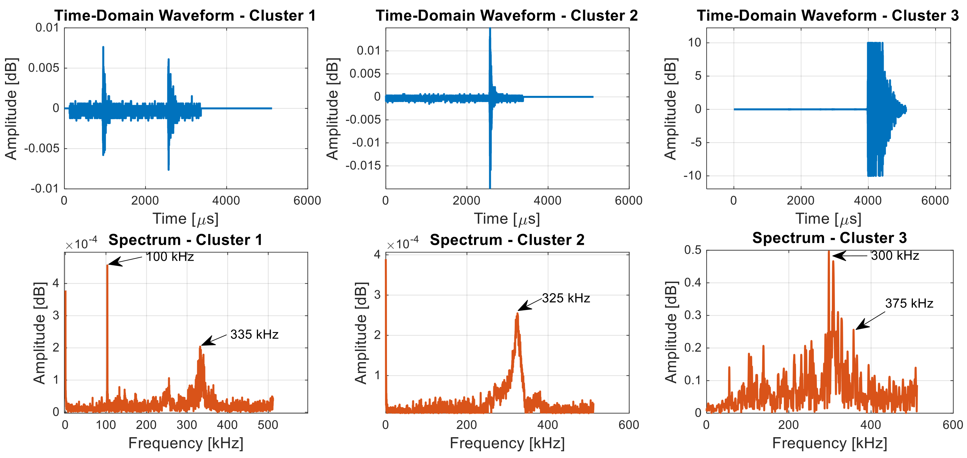
| JLS 1 | 0.01–1.54 | 0.02–1.01 | 0.03–0.8 | 40–48 | 49–65 | 67–100 |
| JLS 2 | 0.03–2.10 | 0.02–1.35 | 0.07–1.03 | 40–58 | 59–78 | 79–100 |
| JLS 3 | 0.01–2.59 | 0.02–1.88 | 0.04–1.52 | 40–53 | 54–75 | 76–100 |
Disclaimer/Publisher’s Note: The statements, opinions and data contained in all publications are solely those of the individual author(s) and contributor(s) and not of MDPI and/or the editor(s). MDPI and/or the editor(s) disclaim responsibility for any injury to people or property resulting from any ideas, methods, instructions or products referred to in the content. |
© 2025 by the authors. Licensee MDPI, Basel, Switzerland. This article is an open access article distributed under the terms and conditions of the Creative Commons Attribution (CC BY) license (https://creativecommons.org/licenses/by/4.0/).
Share and Cite
Barile, C.; Casavola, C.; Katamba Mpoyi, D.; Pappalettera, G. Deep Autoencoder Framework for Classifying Damage Mechanisms in Repaired CFRP. Appl. Sci. 2025, 15, 1209. https://doi.org/10.3390/app15031209
Barile C, Casavola C, Katamba Mpoyi D, Pappalettera G. Deep Autoencoder Framework for Classifying Damage Mechanisms in Repaired CFRP. Applied Sciences. 2025; 15(3):1209. https://doi.org/10.3390/app15031209
Chicago/Turabian StyleBarile, Claudia, Caterina Casavola, Dany Katamba Mpoyi, and Giovanni Pappalettera. 2025. "Deep Autoencoder Framework for Classifying Damage Mechanisms in Repaired CFRP" Applied Sciences 15, no. 3: 1209. https://doi.org/10.3390/app15031209
APA StyleBarile, C., Casavola, C., Katamba Mpoyi, D., & Pappalettera, G. (2025). Deep Autoencoder Framework for Classifying Damage Mechanisms in Repaired CFRP. Applied Sciences, 15(3), 1209. https://doi.org/10.3390/app15031209