
Structural Health Assessment of a Reinforced Concrete Building in Valparaíso Under Seismic and Environmental Shaking: A Foundation for IoT-Driven Digital Twin Systems

 ,
,  ,
,  and
and
Abstract
1. Introduction
Review of the State of the Art
2. Methodology of SSI-COV
2.1. System Model
2.2. Extraction of Modal Characteristics
2.3. Hankel Matrix Parameters: Dimension and Order
2.4. Implementation of SSI-COV
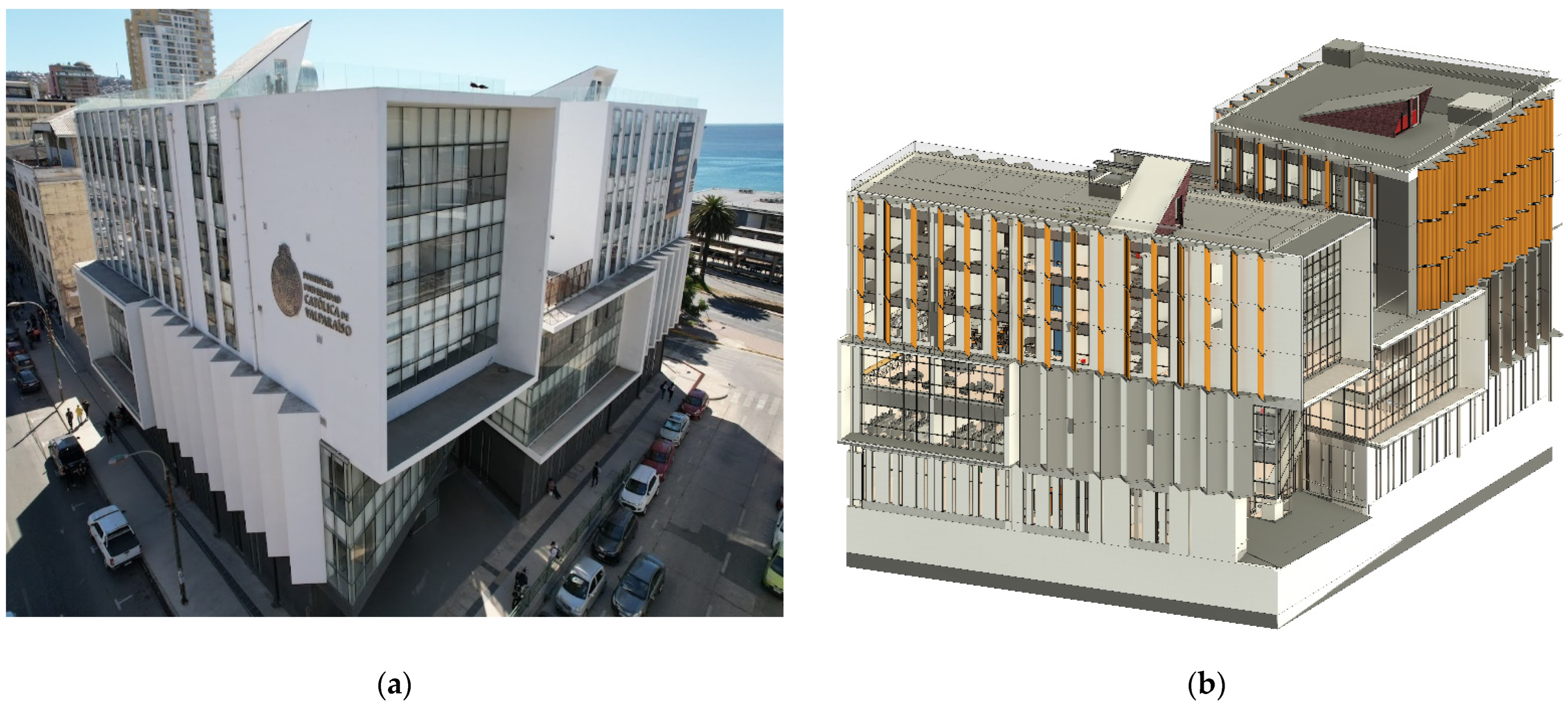
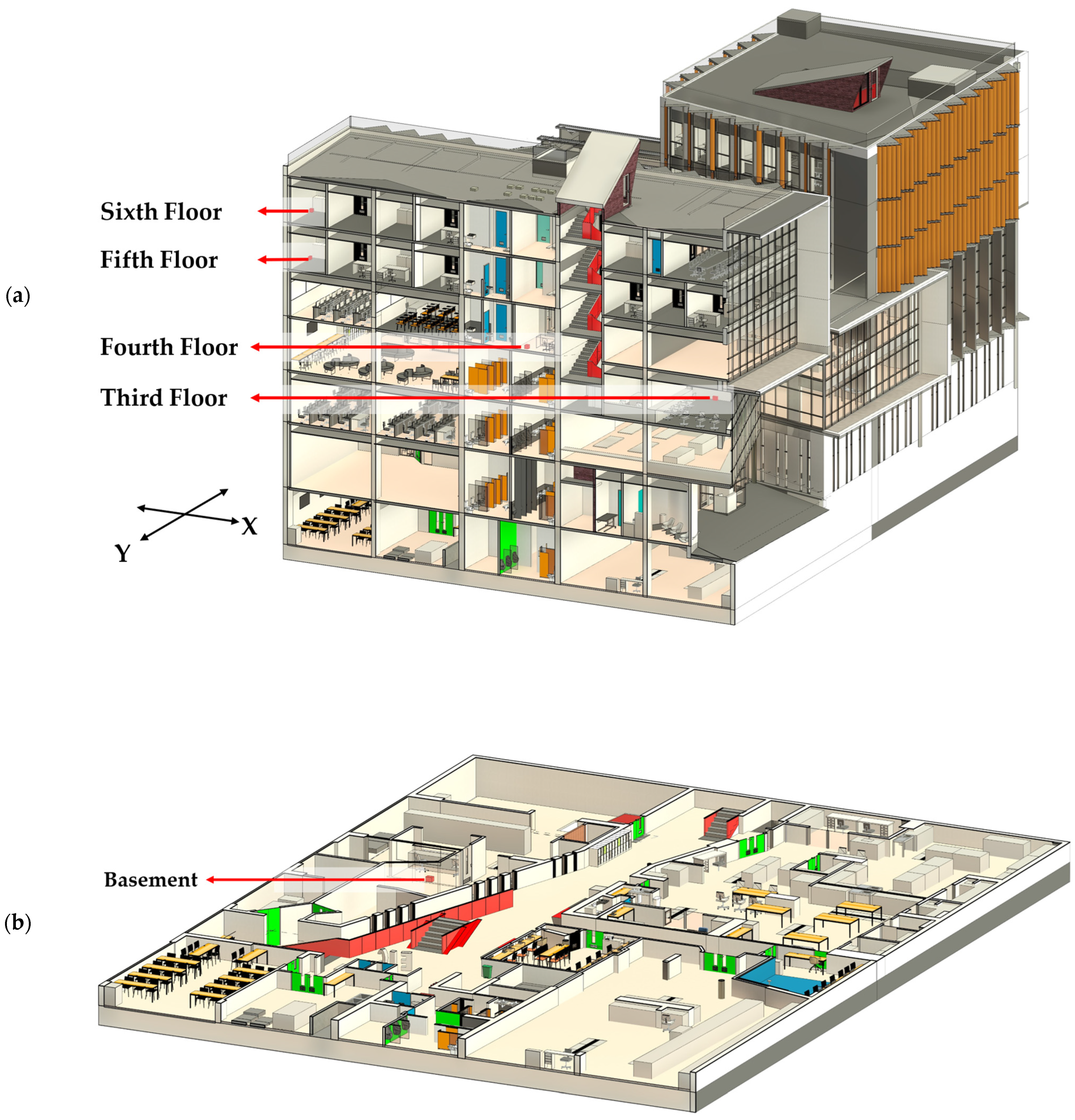
3. Tested Building Description
4. Experimental Procedure
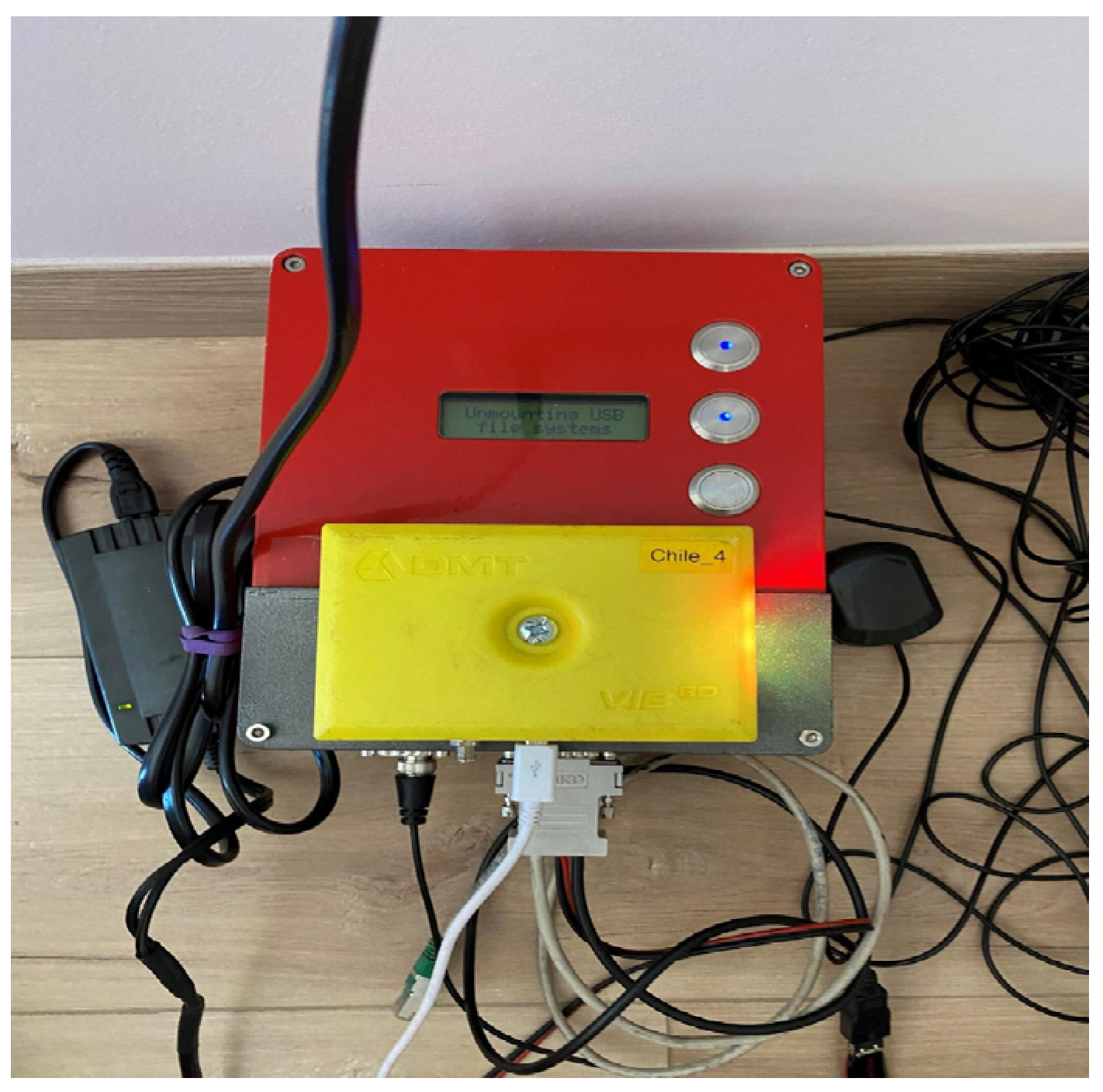
4.1. Instrumentation
4.2. Monitoring Campaign
5. Results
5.1. Ambient Vibration Results for 2022–2023
5.2. Ambient Vibration Results for 2024
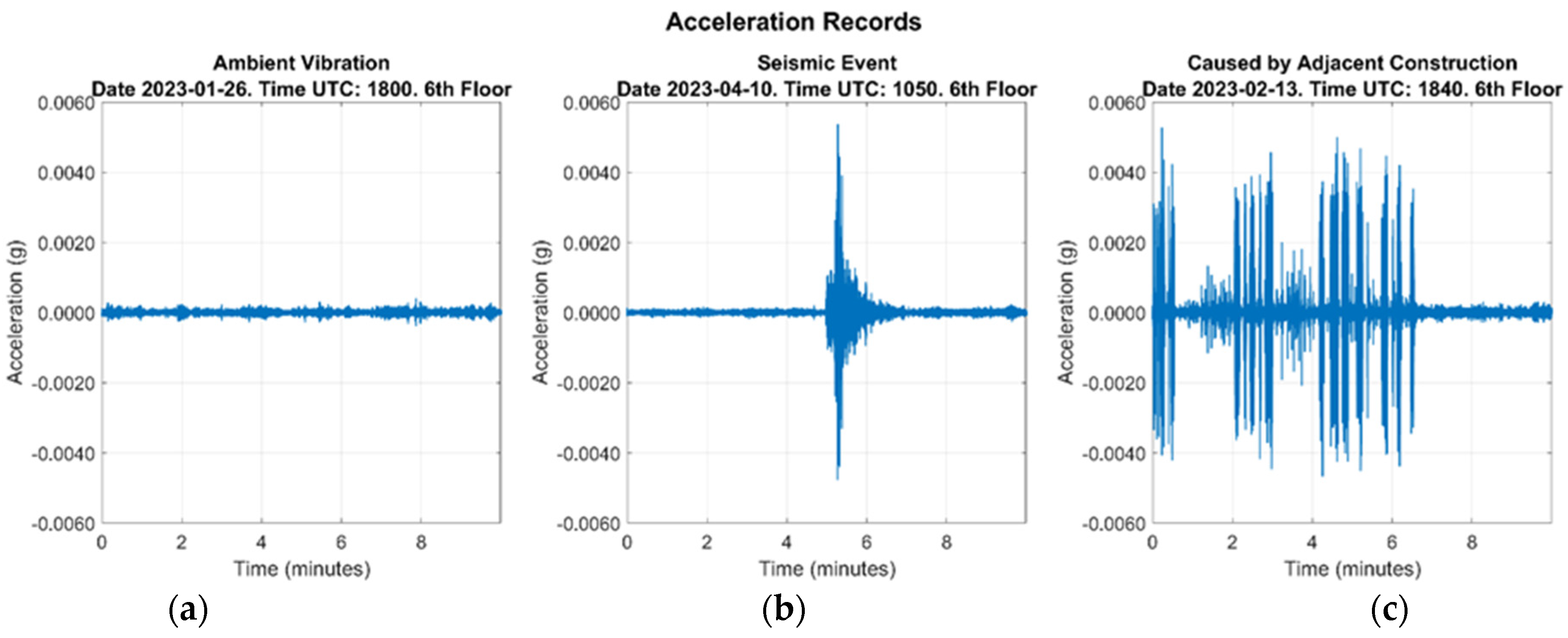
5.3. Seismic Event Results
5.4. Adjacent Construction Activity Results
6. Conclusions
Author Contributions
Funding
Data Availability Statement
Acknowledgments
Conflicts of Interest
References
- Beskhyroun, S.; Navabian, N.; Wotherspoon, L.; Ma, Q. Dynamic behaviour of a 13-story reinforced concrete building under ambient vibration, forced vibration, and earthquake excitation. J. Build. Eng. 2020, 28, 101066. [Google Scholar] [CrossRef]
- Farrar, C.R.; Worden, K. An introduction to structural health monitoring. Phil. Trans. R. Soc. A. 2007, 365, 303–315. [Google Scholar] [CrossRef] [PubMed]
- Chen, H.; Ni, Y. Structural Health Monitoring of Large Civil Engineering Structures, 1st ed.; Wiley: Hoboken, NJ, USA, 2018. [Google Scholar] [CrossRef]
- Avci, O.; Abdeljaber, O.; Kiranyaz, S.; Hussein, M.; Gabbouj, M.; Inman, D.J. A review of vibration-based damage detection in civil structures: From traditional methods to Machine Learning and Deep Learning applications. Mech. Syst. Signal Process. 2021, 147, 107077. [Google Scholar] [CrossRef]
- Zhang, L.; Brincker, R.; Andersen, P. An Overview of Operational Modal Analysis: Major Development and Issues. In Proceedings of the 1st International Operational Modal Analysis Conference (IOMAC 2005), Copenhagen, Denmark, 26–27 April 2005. [Google Scholar]
- Azzara, R.M.; Girardi, M.; Iafolla, V.; Lucchesi, D.M.; Padovani, C.; Pellegrini, D. Ambient Vibrations of Age-old Masonry Towers: Results of Long-term Dynamic Monitoring in the Historic Centre of Lucca. Int. J. Arch. Heritage 2021, 15, 5–21. [Google Scholar] [CrossRef]
- Reynders, E.; Maes, K.; Lombaert, G.; De Roeck, G. Uncertainty quantification in operational modal analysis with stochastic subspace identification: Validation and applications. Mech. Syst. Signal Process. 2016, 66–67, 13–30. [Google Scholar] [CrossRef]
- De Roeck, G. Model–Based Methods of Damage Identification of Structures Under Seismic Excitation. In Seismic Structural Health Monitoring; Limongelli, M.P., Çelebi, M., Eds.; Springer International Publishing: Cham, Switzerland, 2019; pp. 237–259. [Google Scholar] [CrossRef]
- Kamariotis, A.; Chatzi, E.; Straub, D. Value of information from vibration-based structural health monitoring extracted via Bayesian model updating. Mech. Syst. Signal Process. 2022, 166, 108465. [Google Scholar] [CrossRef]
- Zhang, W.; Li, J.; Hao, H.; Ma, H. Damage detection in bridge structures under moving loads with phase trajectory change of multi-type vibration measurements. Mech. Syst. Signal Process. 2017, 87, 410–425. [Google Scholar] [CrossRef]
- Gomes, G.F.; Mendez, Y.A.D.; Alexandrino, P.d.S.L.; da Cunha, S.S.; Ancelotti, A.C. A Review of Vibration Based Inverse Methods for Damage Detection and Identification in Mechanical Structures Using Optimization Algorithms and ANN. Arch. Comput. Methods Eng. 2018, 26, 883–897. [Google Scholar] [CrossRef]
- Zhelyazkov, A.; Wenzel, D.Z.H.; Furtner, P. A Procedure for Post-Earthquake Damage Estimation Based on Detection of High-Frequency Transients. Int. J. Struct. Constr. Eng. 2018, 12, 11. [Google Scholar]
- Samusev, M. Structural Health Monitoring Toolbox (shmtoolbox V.1.2.1). 2024. Available online: https://www.mathworks.com/matlabcentral/fileexchange/68988-shmtoolbox (accessed on 6 March 2022).
- Yin, Z.; Lu, Z.-R.; Liu, J.; Wang, L. Quantifying uncertainty for structural damage identification in the presence of model errors from a deterministic sensitivity-based regime. Eng. Struct. 2022, 267, 114685. [Google Scholar] [CrossRef]
- Gentile, C.; Saisi, A.; Cabboi, A. Structural Identification of a Masonry Tower Based on Operational Modal Analysis. Int. J. Arch. Heritage 2015, 9, 98–110. [Google Scholar] [CrossRef]
- LabSens—PUCV—Structure Health Monitoring. Available online: https://sites.google.com/pucv.cl/labsens/%C3%A1reas-de-trabajo/structure-health-monitoring (accessed on 7 November 2024).
- Toh, G.; Park, J. Review of Vibration-Based Structural Health Monitoring Using Deep Learning. Appl. Sci. 2020, 10, 1680. [Google Scholar] [CrossRef]
- Olivera-López, J.J.; Oyarzo-Vera, C.A. Diagnóstico estructural de un edificio de hormigón armado basado en su perfil bio-sísmico y un análisis dinámico incremental. Obras y Proy. 2020, 27, 95–106. [Google Scholar] [CrossRef]
- Argentino, A.; Bono, F.M.; Bernardini, L.; Romano, N.; Cazzulani, G.; Somaschini, C.; Belloli, M.; Cinquemani, S. Automated OMA Through SSI-COV Algorithm of a Warren Truss Railway Bridge Exploiting Free Decay Response. In Proceedings of the 10th International Operational Modal Analysis Conference (IOMAC 2024); Rainieri, C., Gentile, C., López, M.A., Eds.; Springer Nature: Cham, Switzerland, 2024; pp. 600–608. [Google Scholar] [CrossRef]
- Alustiza, D.H.; López, A.; Mineo, M.; Russo, N.A.; Zaccardi, Y.A.V. Introducción a los Sensores de Fibra Óptica para el Monitoreo de Salud de Estructuras Civiles. 2022. Available online: https://portal.amelica.org/ameli/journal/266/2663014002/ (accessed on 6 November 2024).
- Sivasuriyan, A.; Vijayan, D.S.; Górski, W.; Wodzyński, Ł.; Vaverková, M.D.; Koda, E. Practical Implementation of Structural Health Monitoring in Multi-Story Buildings. Buildings 2021, 11, 263. [Google Scholar] [CrossRef]
- Maas, S.; Nguyen, V.H.; Kebig, T.; Schommer, S.; Zürbes, A. Comparison of different excitation- and data sampling-methods in structural health monitoring. Civ. Eng. Des. 2019, 1, 10–16. [Google Scholar] [CrossRef]
- Jiazeng, J.S.; Changhao, Z.; Xi, C.; Cheng, N.L. Model Updating of a Shear-Wall Tall Building using Various Vibration Monitoring Data: Accuracy and Robustness. Struct. Des. Tall Spéc. Build. 2024, 33, e2114. [Google Scholar] [CrossRef]
- Gartner Mc Bain, L.F.; Minota Zea, Y.M. Evaluación Preliminar del Comportamiento de Láminas de Caucho Reciclado como Elemento de Apoyo en Modelos de Vigas Simplemente Apoyadas Sometidas a Vibraciones Horizontales. Ph.D. Thesis, Universidad Santo Tomás De Aquino Facultad De Ingeniería, Bogotá D.C., Colombia, 2019. Available online: https://1library.co/es/download/881108955325071362 (accessed on 6 November 2024).
- Mancini, A.; Cosoli, G.; Mobili, A.; Violini, L.; Pandarese, G.; Galdelli, A.; Narang, G.; Blasi, E.; Tittarelli, F.; Revel, G.M. A monitoring platform based on electrical impedance and AI techniques to enhance the resilience of the built environment. Acta IMEKO 2024, 13, 1–12. [Google Scholar] [CrossRef]
- Bonekemper, L.; Wiemann, M.; Kraemer, P. Automated set-up parameter estimation and result evaluation for SSI-Cov-OMA. Vibroengineering PROCEDIA 2020, 34, 43–49. [Google Scholar] [CrossRef]
- Maybeck, P.S. (Ed.) Chapter 4 Stochastic processes and linear dynamic system models. In Mathematics in Science and Engineering; Elsevier: Amsterdam, The Netherlands, 1979; pp. 133–202. [Google Scholar] [CrossRef]
- Sun, S.; Yang, B.; Zhang, Q.; Wüchner, R.; Pan, L.; Zhu, H. Fast online implementation of covariance-driven stochastic subspace identification. Mech. Syst. Signal Process. 2023, 197, 110326. [Google Scholar] [CrossRef]
- David, N.N.E.; Cherkaoui, S. Simulation Methods, Techniques and Tools of Computer Systems and Networks. 2024. Available online: https://www.sciencedirect.com/science/article/abs/pii/B9780128008874000171 (accessed on 13 October 2024).
- Miller, D.N.; de Callafon, R.A. Subspace Identification from Classical Realization Methods. IFAC Proc. Vol. 2009, 42, 102–107. [Google Scholar] [CrossRef]
- Pourgholi, M.; Gilarlue, M.M.; Vahdaini, T.; Azarbonyad, M. Influence of Hankel matrix dimension on system identification of structures using stochastic subspace algorithms. Mech. Syst. Signal Process. 2022, 186, 109893. [Google Scholar] [CrossRef]
- Wu, R.-T.; Jahanshahi, M.R. Data fusion approaches for structural health monitoring and system identification: Past, present, and future. Struct. Heal. Monit. 2020, 19, 552–586. [Google Scholar] [CrossRef]
- Tran-Ngoc, H.; Khatir, S.; De Roeck, G.; Bui-Tien, T.; Nguyen-Ngoc, L.; Wahab, M.A. Stiffness Identification of Truss Joints of the Nam O Bridge Based on Vibration Measurements and Model Updating. In Proceedings of ARCH 2019; Arêde, A., Costa, C., Eds.; Springer International Publishing: Cham, Switzerland, 2020; pp. 264–272. [Google Scholar] [CrossRef]
- Rainieri, C.; Fabbrocino, G. Influence of model order and number of block rows on accuracy and precision of modal parameter estimates in stochastic subspace identification. Int. J. Lifecycle Perform. Eng. 2014, 1, 317. [Google Scholar] [CrossRef]
- Li, B.; Liang, W.; Yang, S.; Zhang, L. Automatic identification of modal parameters for high arch dams based on SSI incorporating SSA and K-means algorithm. Appl. Soft Comput. 2023, 138, 110201. [Google Scholar] [CrossRef]
- Pereira, S.; Reynders, E.; Magalhães, F.; Cunha, Á.; Gomes, J.P. The role of modal parameters uncertainty estimation in automated modal identification, modal tracking and data normalization. Eng. Struct. 2020, 224, 111208. [Google Scholar] [CrossRef]
- Ruggieri, S.; Bruno, G.; Attolico, A.; Uva, G. Assessing the dredging vibrational effects on surrounding structures: The case of port nourishment in Bari. J. Build. Eng. 2024, 96, 110385. [Google Scholar] [CrossRef]
- Zhang, F.; Ni, Y.; Lam, H. Bayesian structural model updating using ambient vibration data collected by multiple setups. Struct. Control Heal. Monit. 2017, 24, e2023. [Google Scholar] [CrossRef]
- Song, M.; Behmanesh, I.; Moaveni, B.; Papadimitriou, C. Hierarchical Bayesian Calibration and Response Prediction of a 10-Story Building Model. In Model Validation and Uncertainty Quantification; Barthorpe, R., Ed.; Springer International Publishing: Cham, Switzerland, 2019; Volume 3, pp. 153–165. [Google Scholar] [CrossRef]


| Mode | Frequency HZ | UX % | UY% |
|---|---|---|---|
| 1 | 1.94 | 1.94 | 0.01 |
| 2 | 2.24 | 63.07 | 0.61 |
| 3 | 2.74 | 0.36 | 66.31 |
| 4 | 7.30 | 1.87 | 0 |
| 5 | 9.34 | 14.38 | 1.32 |
| 6 | 10.10 | 1.19 | 17.94 |
| Parameters | Numerical Value |
|---|---|
| Standard range | 2 G |
| ADC resolution | 32 bits |
| Dynamic range | 144 dB |
| Sampling frequency | 400 HZ |
Disclaimer/Publisher’s Note: The statements, opinions and data contained in all publications are solely those of the individual author(s) and contributor(s) and not of MDPI and/or the editor(s). MDPI and/or the editor(s) disclaim responsibility for any injury to people or property resulting from any ideas, methods, instructions or products referred to in the content. |
© 2025 by the authors. Licensee MDPI, Basel, Switzerland. This article is an open access article distributed under the terms and conditions of the Creative Commons Attribution (CC BY) license (https://creativecommons.org/licenses/by/4.0/).
Share and Cite
Lozano-Allimant, S.; Lopez, A.; Gomez, M.; Atencio, E.; Lozano-Galant, J.A.; Fingerhuth, S. Structural Health Assessment of a Reinforced Concrete Building in Valparaíso Under Seismic and Environmental Shaking: A Foundation for IoT-Driven Digital Twin Systems. Appl. Sci. 2025, 15, 1202. https://doi.org/10.3390/app15031202
Lozano-Allimant S, Lopez A, Gomez M, Atencio E, Lozano-Galant JA, Fingerhuth S. Structural Health Assessment of a Reinforced Concrete Building in Valparaíso Under Seismic and Environmental Shaking: A Foundation for IoT-Driven Digital Twin Systems. Applied Sciences. 2025; 15(3):1202. https://doi.org/10.3390/app15031202
Chicago/Turabian StyleLozano-Allimant, Sebastián, Alvaro Lopez, Miguel Gomez, Edison Atencio, José Antonio Lozano-Galant, and Sebastian Fingerhuth. 2025. "Structural Health Assessment of a Reinforced Concrete Building in Valparaíso Under Seismic and Environmental Shaking: A Foundation for IoT-Driven Digital Twin Systems" Applied Sciences 15, no. 3: 1202. https://doi.org/10.3390/app15031202
APA StyleLozano-Allimant, S., Lopez, A., Gomez, M., Atencio, E., Lozano-Galant, J. A., & Fingerhuth, S. (2025). Structural Health Assessment of a Reinforced Concrete Building in Valparaíso Under Seismic and Environmental Shaking: A Foundation for IoT-Driven Digital Twin Systems. Applied Sciences, 15(3), 1202. https://doi.org/10.3390/app15031202