GeoSAE: A 3D Stratigraphic Modeling Method Driven by Geological Constraint

Abstract

Deep learning outperforms traditional interpolation methods in 3D geological modeling due to its ability to model nonlinear relationships and its flexibility in incorporating diverse geological data. However, acquiring geological data for practical applications is challenging, and the quality of the data can vary significantly, which limits the effectiveness of purely data-driven deep learning models in 3D geological modeling. To address this challenge, this paper introduces GeoSAE, a geoconstraint-driven 3D geological modeling method. GeoSAE improves potential field prediction by employing a stacked autoencoder network (SAE) and incorporating geological constraints as a loss function during model training. This approach generates a geologically consistent, smooth, and continuous 3D stratigraphic model. To validate the method, this study applies it to a 60-square-kilometer region in Jiangdong new district, Haikou city, China. Stratigraphic interface points were utilized to predict the 3D potential field, with PyVista (version 0.44.2) enabling the accurate extraction of stratigraphic interfaces. Model quality was evaluated through comprehensive assessments of loss function analysis, data fitting, and the verification of stratigraphic smoothness constraints. Results indicate that the stratigraphic model generated by GeoSAE closely aligns with the actual data, accurately capturing stratigraphic geometry. Additionally, incorporating smoothness constraints enhances model smoothness, minimizes irregular stratigraphic fluctuations, and produces a more natural and continuous stratigraphic morphology.

1. Introduction

Currently, geological modeling methods across various geological formations and applications are being gradually refined and made more comprehensive. Three-dimensional geological modeling is mainly categorized into explicit modeling, implicit modeling [1,2], and deep learning-based modeling, with greater attention being given to the latter due to advances in machine learning.

(1)

Geological and geophysical knowledge is relied upon in traditional explicit modeling methods to construct geological interfaces, with data from geological maps, boreholes, and geological cross-sections being utilized [3]. The quality of the model is significantly influenced by the accuracy of the interpreted data. Each stratigraphic surface is explicitly modeled, and constrained grid interpolation is employed to refine the model and generate more detailed surfaces [4]. Additionally, semi-automated, interactive methods are employed to enable the manual addition of geological constraints [5,6,7], ensuring better alignment with geological knowledge. Various interpolation methods, including Bézier curve interpolation [8], non-uniform rational B-Spline (NURBS) interpolation [9], and the discrete smoothing interpretation (DSI) method introduced by J. Mallet in 2002 [10,11], have been proposed to better fit geological observations and adapt to different geological structures.

Although complex, well-constrained models can be produced by explicit 3D geological modeling, the incorporation of geological constraints is time-consuming and labor-intensive, requiring substantial modeling expertise and geological knowledge. Moreover, the process is difficult to reproduce and is prone to topological errors, such as voids and self-intersections, which hinder the widespread application of 3D geological models in practical production environments [5].

(2)

Isosurfaces traced from a 3D potential field are used in implicit modeling to represent geological interfaces [12], and discrete geological data—such as interface points and structural observations—are interpolated using implicit functions [13]. Various implicit modeling methods have been proposed, with different mathematical frameworks being employed, including Kriging-based implicit modeling [14,15], discrete smoothing interpolation (DSI) [16], and radial basis function (RBF) methods [17,18].

Advantages in grid quality, reproducibility, and dynamic updating are provided by implicit modeling when compared to explicit methods [19]. However, modeling artifacts may be introduced in regions with complex geological structures. To resolve these artifacts, spatial relationships between geological history and features are incorporated as constraints into the implicit modeling process, forming a hybrid implicit–explicit approach [20,21]. However, reduced reproducibility and modeling efficiency can result from this approach.

(3)

Intrinsic geological features are mined from large geological data samples through training with different learning paradigms in deep learning methods. Geological prior knowledge is incorporated to explore geological expressions that align with geological laws, observations, and structural anisotropy. Various 3D geological modeling methods based on deep learning are being continuously explored. Classification algorithm-based networks, such as support vector machines and BP neural networks, are employed to automate the construction of 3D geological models from borehole data [22]. Semantic mining is performed using recurrent neural networks (RNNs), where the prediction of stratum types and layer thicknesses is simulated [23]. Three-dimensional geological model parameters are inverted from geophysical data using convolutional neural networks (CNNs), and geological datasets are synthesized [24]. Generative adversarial networks (GANs), including variants such as deep convolutional generative adversarial networks (DCGAN) and Monte Carlo simulation-based GANs (MC-GAN), have been proposed to improve 3D geological modeling [25,26,27]. Reliable 3D geological models are constructed by combining drill holes, outcrops, and 2D geological cross-sections as strong constraints in these methods. Stochastic processes are modeled, and scale conversion is facilitated in these methods, while geological observations are integrated into graph structures using graph neural networks (GNNs), thereby extending the range of constraints [28]. Geological constraints are often added to the inversion function or applied during post-processing of the inversion model after each inversion step to align it with geological characteristics in the construction of 3D geological models with geological constraints [29]. For specific geological formations, seismic voxels are used to estimate relative geologic time (RGT) for stratigraphy interpretation and fault detection, and fault models consistent with geological structures are generated [30]. However, the modeling of non-integrated structures is still considered difficult. A framework combining deep learning with implicit modeling has recently been proposed to improve the application of implicit methods in structural geology, with a multilayer perceptron (MLP) architecture being utilized [31].

Despite considerable progress in research, significant limitations are faced in the practical application of deep learning-based 3D geological modeling methods. The data required for 3D geological modeling are typically scarce and difficult to obtain, contradicting deep learning’s reliance on large datasets. Consequently, the extraction of more features from sparse data has become a significant challenge in applying deep learning methods to 3D geological modeling. The construction of 3D geological models requires the consideration of complex geological bodies, and the data scale is often large. High-precision models necessitate significant computational resources, presenting challenges for deep learning networks, computational methods, optimization algorithms, and hardware performance. The non-visible nature of underground spaces introduces uncertainty in the mechanisms of deep learning models, making it difficult to provide reliable explanations or practical support for the generated 3D geological models.

The design of a suitable neural network capable of capturing the intrinsic features and distribution patterns of geological data is a key step in using deep learning for 3D geological modeling, allowing geological structures in uncharted areas to be inferred [32]. In this study, an auto-encoder (AE) is used to learn feature representations of a dataset through network training, and the original data is subsequently reconstructed from these features. For 3D geological modeling, useful features are learned from the input data by the auto-encoder during training, which can be applied to tasks such as constructing 3D potential fields, noise reduction, and classification [33]. Furthermore, incomplete input data can be accommodated by the auto-encoder’s decoder, offering advantages in handling missing data in 3D potential fields and proving particularly suitable for sparse and heterogeneous geological data inputs.

The analysis above highlights the critical issue of insufficient constraints related to geological evolution in the construction of 3D geological models, which remains an urgent challenge in the field of 3D geological modeling. To address this challenge, this work presents GeoSAE, a geological constraint-driven 3D modeling method that incorporates geological constraints into the modeling process. In GeoSAE, the “S”, “A”, and “E” represent Stacked Autoencoder, which is a neural network architecture where multiple autoencoders are stacked to simultaneously predict several potential field values.

2. Methods

2.1. Geologically Constrained Loss Function Construction

The model’s interpretability is enhanced by incorporating geological knowledge as constraints in 3D geological modeling. In traditional 3D geological modeling methods, models that do not conform to geological laws are typically corrected through manual adjustments, which is a process that is not only hard to reproduce but also involves high labor costs. However, in deep learning, the deviation between the predicted model and the true model can be quantified by the inversion process based on loss functions, providing direct guidance for model training. New opportunities for integrating geological constraints are opened up by this feature. By expressing geological knowledge mathematically as part of the loss function, the adherence of the output model to geological principles can be ensured. Furthermore, various geological constraints with different loss terms can be combined within a multi-task learning framework, balancing their influence and improving the model’s generalization ability and interpretability.

In response, various geological constraints are effectively transformed into inequality forms in this approach, enabling the precise mathematical expression of geological knowledge and opening new pathways for the effective integration of geological constraints into 3D geological modeling. Details on how to construct corresponding loss functions for a variety of geological constraints will be provided in the following section. Moreover, the model’s adaptability and accuracy in complex geological environments are enhanced by dynamically adjusting the weights of the loss function based on geological conditions.

2.1.1. Consistency Constraints on Sampling Points of Stratigraphic Surfaces

The stratigraphic surface $I_K$ is sampled at the point set $K$, with corresponding potential field values $S_K^{I_K}$ and a variance near 0 [34], ensuring that all points in this set lie on the same potential field surface. This results in a fitted potential field that more closely represents the true conditions of the stratigraphic surface, as expressed in Equation (1):

$$Var(S_K^{I_K})=0$$

(1)

Here, the set of potential field values for the sampled point set $K$ of the stratigraphic surface $I_K$, denoted as $S_K^{I_K}$, is represented within the potential field associated with $I_K$.

The stratigraphic surface sampling point consistency constraint is formulated as a loss function, with the sum of the variances of the potential field values for all stratigraphic surfaces being used, as shown in Equation (2):

$$Los{s}_I^{Var}={\Sigma }_{I_K\in I}^{\left|I\right|}Var(S_K^{I_K})$$

(2)

Here, the total number of stratigraphic surfaces is represented by $\left|I\right|$, and a specific potential field is denoted by $I_K$.

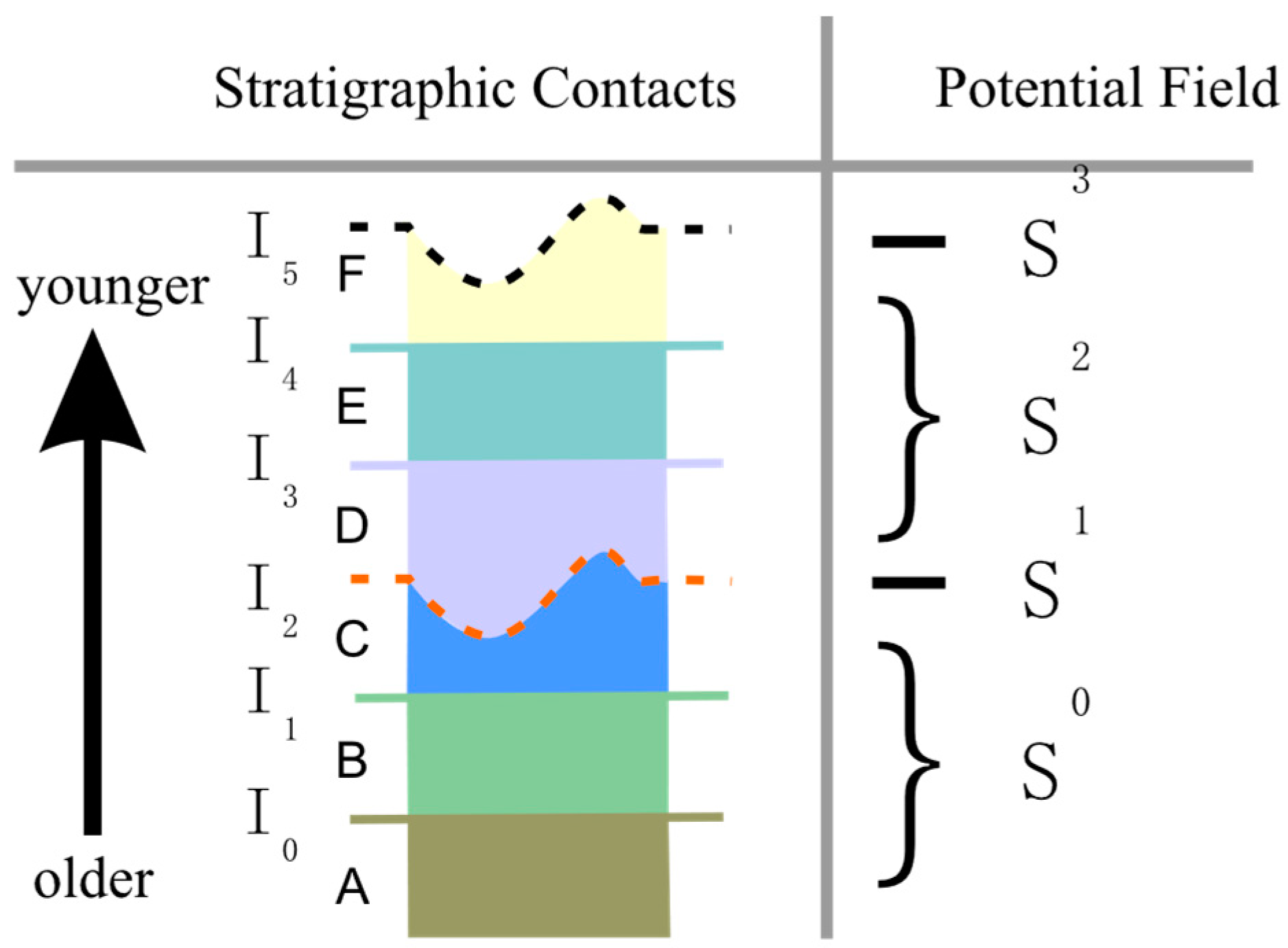
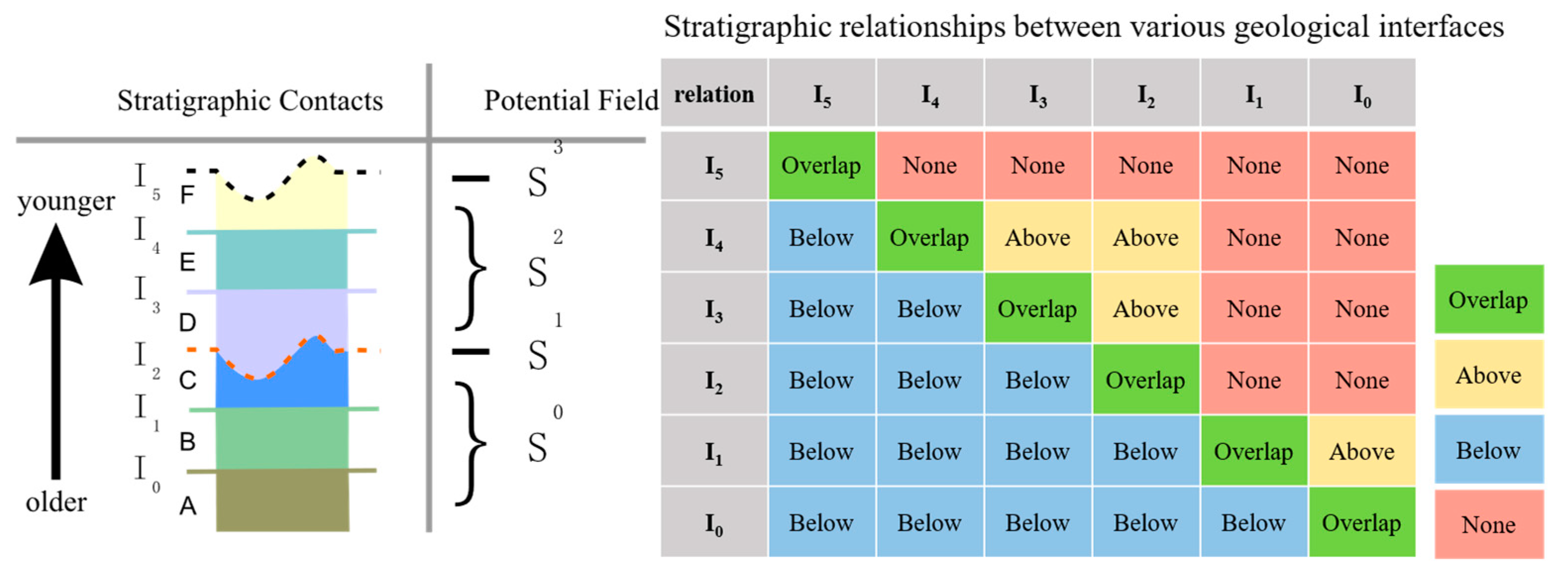
2.1.2. Stratigraphic Sequence Constraints

In 3D geological modeling, the spatial distribution of strata is commonly represented by using the potential field method, which involves defining potential fields. The appropriate number of potential fields is determined based on the stratigraphic contact relationships, ensuring that the morphological characteristics of each stratigraphic surface are accurately captured. The stratigraphic contact relationship is determined through geological field observations, combined with the stratigraphic age relationship, and represented on the stratigraphic column. If two strata are in contact, share the same depositional environment, and exhibit integrated properties, they are represented by the same potential field due to their similar stratigraphic characteristics. Conversely, if there is an unconformity or significant depositional difference between the strata, each unconformity is assigned its own potential field to ensure that the geological features are accurately reflected in the model, as shown in Figure 1. In Figure 1, six stratigraphic surfaces are shown, including two unconformable interfaces ($I_2$ and $I_5$) and four conformable interfaces ($I_0$, $I_1$, $I_3$, and $I_4$). These are modeled by constructing four potential fields based on the stratigraphic contact relationships. The stratigraphic surfaces and units correspond to potential fields as follows: potential field $S_0$ is associated with stratigraphic surfaces $I_0$, $I_1$, and units $A$, $B$, and $C$; potential field $S_1$ is associated with stratigraphic surface $I_2$; potential field $S_2$ is associated with stratigraphic surfaces $I_3$, $I_4$, and units $D$, $E$, and $F$; and potential field $S_3$ is associated with stratigraphic surface $I_5$.

Based on the vertical relationships between strata, the relative magnitude of the potential field values corresponding to sampling points at different stratigraphic surfaces within the same potential field can be inferred. The following definitions are provided in this paper:

“Above” relationship: For a given potential field representing consecutive strata, the potential field value at the sampling point of the upper stratum is required to be greater than that of the lower stratum if one stratum is above another.

“Below” relationship: In all potential fields, the potential field value at the sampling point of the lower stratum is required to be less than that of the upper stratum if one stratum is beneath another.

“Overlap” relationship: If two stratigraphic surfaces overlap, equality of the potential field values at the sampling points along the interface of these strata is required.

The “above” relationship is applied only within the same potential field because an unconformity is introduced by contact between strata from different potential fields. In this situation, the upper strata are influenced by the older strata beneath them, creating an erosional contact. Consequently, the potential field value of the upper strata may be lower than that of the lower strata due to the erosive effects on the older strata, as illustrated in Figure 2b. In the eroded portion of stratum $I_2$ at the unconformity, the potential field value at the sampling point of stratum $I_2$ is smaller than that of stratum $I_1$, indicating that the “above” relationship does not apply in this case. However, the “below” relationship is unaffected. If one stratum is beneath another, the potential field values at the sampling points in the lower stratum must always be less than those in the upper stratum for the “below” relationship to hold.

Therefore, based on the definitions of the “above”, “below”, and “overlap” relationships, an example of the layer ordering relationships based on potential field values between the various stratigraphic layers in Figure 1 is illustrated in Figure 3.

The relationships of “above”, “below”, and “overlap” between layers at each location are determined based on potential field values, and corresponding loss functions are constructed as outlined below.

For each stratigraphic surface, the difference between the potential field value $S_x^{I_X}$ of any point $x$ in the sampling set $X$ of stratigraphic surface $I_K$ and the average potential field value $\overline{S_K^{I_K}}$ of stratigraphic surface $I_K$ is used to indicate the following: if the difference $D_{I_x,I_K}$, $I_K$ is greater than 0, point $x$ is considered to be above stratigraphic surface $I_K$; if the difference $D_{I_x,I_K}$ is less than 0, point $x$ is considered to be below stratigraphic surface $I_K$; and if the difference $D_{I_x,I_K}$ is equal to 0, point $x$ is considered to be on stratigraphic surface $I_K$, meaning the two overlap. The relevant formula is as follows.

The hierarchical relationship between the surfaces is represented by the constraint inequality provided in Equation (3):

$$\begin{array}{l}{D}_{I_x,I_K}>0\to Above\\ D_{I_x,I_K}<0\to Below\\ D_{I_x,I_K}=0\to Overlap\end{array}$$

(3)

where the difference in potential field between stratigraphic surfaces, denoted as $D_{I_x,I_K}$, is given by Equation (4):

$$D_{I_x,I_K}=S_x^{I_X}-\overline{S_K^{I_K}}$$

(4)

where the potential field value of point $x$ within the potential field at stratigraphic surface $I_X$ is represented by $S_x^{I_X}$, and the average potential field value at stratigraphic surface $I_X$ is denoted by $\overline{S_K^{I_K}}$, as shown in Equation (5):

$$\overline{S_K^{I_K}}={\displaystyle \frac{1}{\left|K\right|}}\sum S^{I_K}(K)={\displaystyle \frac{1}{\left|K\right|}}{\sum }_{k\in K}^{\left|K\right|}{S}_k^{I_K}$$

(5)

The number of points in the sampling point set $K$ at the stratigraphic surface $I_K$ is represented by $\left|K\right|$, with $k$ being one of the sampled points in the set. If the difference $D_{I_x,I_K}$ between the potential field value $S_x^{I_X}$ at point x and the average potential field value $\overline{S_K^{I_K}}$ at stratigraphic surface $I_K$ is non-zero, the loss of the average potential field value $\overline{S_K^{I_K}}$ at point $x$ relative to the stratigraphic surface $I_K$ is represented by the approximate signed distance ${\delta }_{I_x,I_K}$. The relevant formulae are presented as follows.

The formula for the approximate signed distance ${\delta }_{I_x,I_K}$ is given in Equation (6):

$${\delta }_{I_x,I_K}={\displaystyle \frac{D_{I_x,I_K}}{‖\nabla S_x^{I_X}‖}}={\displaystyle \frac{S_x^{I_X}-\overline{S_K^{I_K}}}{‖\nabla S_x^{I_X}‖}}$$

(6)

The scalar gradient of point $x$ in the potential field corresponding to the stratigraphic surface $I_X$ is denoted by $‖\nabla S_x^{I_X}‖$. The change in thickness between the units of interest is represented; a smaller scalar gradient is indicated for thicker units, while a larger gradient is related to thinner units. The approximate signed distance ${\delta }_{I_x,I_K}$ is provided as a more accurate measure of how far a point is above, below, or overlapping with a reference interface compared to the scalar difference $D_{I_x,I_K}$.

The loss function formulae for the layer ordering relationships between surfaces are presented in Equations (7)–(9).

$$L{\mathrm{oss}}_I^{Above}={\sum }_{I_X\in I}^{\left|I\right|}{\displaystyle \frac{1}{\left|X\right|}}{\sum }_{x\in X}^{\left|X\right|}{\sum }_{k\in K}^{\left|K\right|}{\delta }_{I_x,I_K},{\delta }_{I_x,I_K}=\left\{\begin{array}{ll}{\displaystyle \frac{\left|S_x^{I_X}-\overline{S_K^{I_K}}\right|}{‖\nabla S_x^{I_X}‖}}\hfill & S_x^{I_X}-\overline{S_K^{I_K}}<0\hfill \\ 0\hfill & S_x^{I_X}-\overline{S_K^{I_K}}\ge 0\hfill \end{array}\right.$$

(7)

$$Los{s}_I^{Below}={\sum }_{I_X\in I}^{\left|I\right|}{\displaystyle \frac{1}{\left|X\right|}}{\sum }_{x\in X}^{\left|X\right|}{\sum }_{k\in K}^{\left|K\right|}{\delta }_{I_x,I_K},{\delta }_{I_x,I_K}=\left\{\begin{array}{ll}{\displaystyle \frac{\left|S_x^{I_X}-\overline{S_K^{I_K}}\right|}{‖\nabla S_x^{I_X}‖}}\hfill & S_x^{I_X}-\overline{S_K^{I_K}}>0\hfill \\ 0\hfill & S_x^{I_X}-\overline{S_K^{I_K}}\le 0\hfill \end{array}\right.$$

(8)

$$Los{s}_I^{Overlap}={\sum }_{I_X\in I}^{\left|I\right|}{\displaystyle \frac{1}{\left|X\right|}}{\sum }_{x\in X}^{\left|X\right|}\left|{\delta }_{x,I_K}\right|$$

(9)

The total loss for each stratigraphic surface in the above and below relationship is calculated by summing the approximate signed distances of all points in the sampling set $X$ of a given surface $I_X$ to the mean potential field values of all other surfaces. The above and below relationship loss is represented by this sum. For the overlap relationship, the approximate signed distances of all points in the sampling set $X$ of a given stratigraphic surface $I_X$ are summed to the mean potential field value of another surface $I_K$. This represents the overlap relationship loss between the surfaces. Here, $\left|I\right|$ is used to represent the total number of stratigraphic surfaces, $\left|X\right|$ represents the number of points in the sampling set $X$, and $\left|K\right|$ represents the number of stratigraphic surfaces minus one (excluding the current surface).

In summary, the loss function for the stratigraphic relationship between surfaces is expressed in Equation (10):

$$Los{s}_I=Los{s}_I^{Above}+Los{s}_I^{Below}+Los{s}_I^{Overlap}$$

(10)

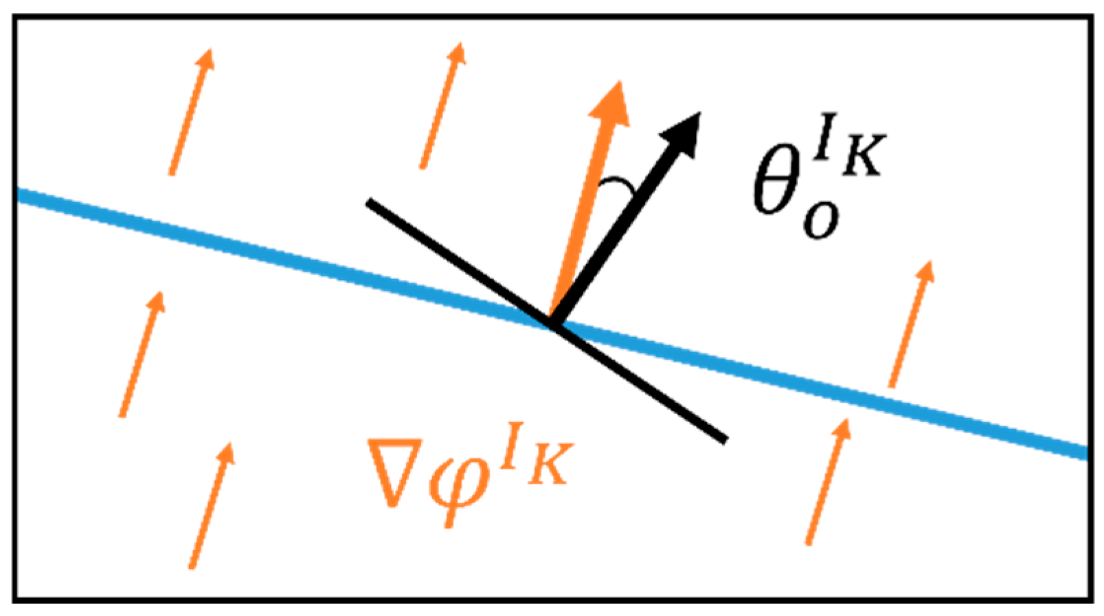
2.1.3. Attitude Constraints on Attitude Points

The spatial geometric features of strata, including structural orientation, dip, and dip direction, are described by the attitude. For the potential field $S^{I_K}$ related to the stratigraphic surface $I_K$, attitude points $O$ are defined on the surface, with each point $o$ belonging to $O$. At this point $o$, the angle ${\theta }_o^{I_K}$ between the actual attitude direction vector and the potential field gradient is used to indicate the angular constraint for the attitude point, as illustrated in Figure 4. In this figure, the trend of the potential field surface $S^{I_K}$ is shown by the blue line, the gradient of the potential field at point $o$ is represented by the orange arrow, and the actual attitude direction vector at point $o$ is denoted by the black cross-arrow. The difference between the actual attitude direction vector and the potential field gradient is measured by the angle ${\theta }_o^{I_K}$. When the attitude direction vector and the potential field gradient at point $o$ are closely aligned (i.e., angle ${\theta }_o^{I_K}$ approaches 0°), a strong attitude constraint in the constructed potential field at point $o$ is signified.

The corresponding equation is as follows:

$${\theta }_o^{I_K}=0^{\circ }$$

(11)

Here, the angle is used to represent the angle between the direction vector at point $o$ and the gradient of the potential field associated with stratigraphic surface, where point $o$ is part of the sampling point set at the stratigraphic surface.

Therefore, when angle ${\theta }_o^{I_K}$ between the attitude direction vector at point $o$ and the potential field gradient is not 0°, the loss between the potential field gradient and the potential field trend at point $o$ within the potential field associated with stratigraphic surface $I_K$ is represented by the cosine of this angle. The corresponding equation is provided below.

The formula for the cosine of angle ${\theta }_o^{I_K}$ is given in Equation (12):

$$\cos {\theta }_o^K={\displaystyle \frac{v_O\cdot \nabla S_O^{I_K}}{‖v_O‖‖\nabla S_O^{I_K}‖}}$$

(12)

The design of the loss function incorporating the attitude direction constraints at the attitude points is presented in Equation (13):

$$L_O={\displaystyle \sum _{K\in F}^F\frac{1}{\left|O\right|}}{\displaystyle \sum _{o\in O}^{\left|O\right|}\left|\cos {\theta }_o-\cos {\theta }_o^K\right|}$$

(13)

The attitude point-related loss is calculated by finding the difference between the cosine of the angle between the actual attitude direction vector and the potential field direction, and the cosine of the angle between the potential field gradient and the potential field direction, for all potential fields containing attitude points. The attitude point-related loss is computed by first averaging the values for the direction point set $O$ in each potential field, and then summing the averages across all $F$ potential fields. Here, $F$ is used to denote the number of potential fields, and $\left|O\right|$ represents the number of attitude points in each potential field’s direction point set.

2.1.4. Stratigraphic Interface Smoothness Constraints

Abrupt changes in the local potential field can be caused by the implicit modeling method when modeling complex geological structures, resulting in discontinuities or unrealistic bumps at stratigraphic surfaces, and modeling artifacts may also be introduced when multiple strata overlap. To address this issue, the energy minimization principle is applied to globally constrain the modeling region, ensuring continuity at stratigraphic interfaces and preventing abrupt changes. In this approach, a unit norm constraint, the Eikonal constraint [35], is utilized. The constraint is defined as a set of points $X$ sampled from the modeling region ${\Omega }_X$, where the gradient of the potential field at each point $x$ is required to be close to the unit paradigm value. A smaller difference between the two is ensured to provide better class-near-parallel characteristics of the nearby strata, promoting smoothness and continuity in the potential field values.

The unit norm constraint formula is shown in Equation (14):

$$‖\nabla S^{{\Omega }_X}(x)‖=1$$

(14)

The potential field of the modeling region ${\Omega }_X$ is represented by $S^{{\Omega }_X}(x)$, where the potential field value at any point $x$ within the sampled point set $X$ is indicated by $S^{{\Omega }_X}(x)$. The gradient of the potential field at point $x$ is referred to by $\nabla S^{{\Omega }_X}(x)$, while the unit norm of the potential field gradient at point $x$ within the sampled point set $X$ is denoted by $‖\nabla S^{{\Omega }_X}(x)‖$.

The stratigraphic interface smoothness constraint loss function is given by Equation (15):

$$L_{\xi }={\Sigma }_{X\in F}^F{\displaystyle \frac{1}{\left|{\Omega }_X\right|}}\left(\left|‖\nabla S^{{\Omega }_X}(x)‖-1\right|\right)$$

(15)

The difference between the gradient of the potential field and the unit norm (i.e., 1) at each point $x$ in the sampling point set $X$ for all $F$ modeling regions is calculated by the global smoothing loss function. This difference is then averaged for each modeling region’s potential field, and the sum of these averages is used to represent the global relevant loss. Here, the number of potential fields in the modeling region is denoted by $F$, and the number of points in the sampling set $X$ for the potential field in the modeling region ${\Omega }_X$ is referred to by $\left|{\Omega }_X\right|$.

2.1.5. Total Loss Function

The total loss, or the combined loss from all the aforementioned geological constraints, is expressed in Equation (16):

$$Loss=Los{s}_I^{Var}+Los{s}_I+Los{s}_O+\lambda Los{s}_{\xi }$$

(16)

The sequence of loss functions, from left to right, includes stratigraphic consistency, stratigraphic sequence relationships, direction constraints at yielding points, and stratigraphic interface smoothness. The stratigraphic interface smoothness loss function is weighted by $\lambda$; a higher $\lambda$ value results in a smoother, more continuous stratigraphic surface.

2.2. Stacked Autoencoder Network Framework

2.2.1. Stacked Autoencoder Network Construction

A network model for predicting the 3D potential field is presented in this work, built from stacked autoencoders with an encoder–decoder structure. Each autoencoder consists of an encoder–decoder structure, as shown in Figure 5, where the encoder is composed of two convolutional layers with kernel sizes of 3 × 128 and 128 × 256, followed by a fully connected layer of 256 × 256. The decoder is composed of two convolutional layers with kernel sizes of 256 × 128 and 128 × 1. The convolutional layers are used with a kernel size of 1 and a stride of 1, ensuring that the input tensor’s dimensions are preserved while producing output tensors with the same height and width but varying channel depth.

A parametric Softplus function is used as the activation function, as shown in Equation (17). The smoothness of the modeled interface is controlled by the parameter $\beta$: smaller $\beta$ values result in flatter interfaces, while larger $\beta$ values are used to emphasize local details.

$$\sigma (x)={\displaystyle \frac{1}{\beta }}\log (1+e^{\beta x})$$

(17)

Complex stratigraphic structures, including successive consolidated and unconformable layers, are often included in real geological data, with each layer having its own implicit potential field ${\phi }^i(i\in F)$. To model $F$ potential fields, $F$ stacked autoencoders are used, where the corresponding $F$ potential field values are generated by each input coordinate point (x, y, z). The network architecture is shown in Figure 6.

2.2.2. Stacked Autoencoder Network Training Framework

The training process for the stacked autoencoder network described in this paper is divided into two stages: geometric initialization of the network variables, followed by the training of the model on a real dataset.

The process of initializing parameters, such as weight matrices, using geometric properties is referred to as geometric initialization of network variables. In this study, the model was designed to represent stratigraphic surfaces, so the output potential field generated by the initialized network variables was required to reflect a reasonable initial geometry for these surfaces. This requirement was addressed by pre-training the network with the provided data. Various geometric initialization methods, including orthogonal, unit circle, and spherical initializations, were used. For stratigraphic modeling, planar initialization was applied during the pre-training process, while spherical initialization was applied for intrusion-like structures. Therefore, this work focuses primarily on planar initialization methods for stratigraphic surfaces. The planar geometry used for pre-training is shown in Figure 7.

Four parallel square planes, with strata labeled 0, 25, 50, and 75 from bottom to top, are included in the pre-training dataset. Planar constraints are learned from these planes, allowing model parameters to be optimized for more efficient training. Reproducibility is ensured during the pre-training process by initializing the network with consistent parameters rather than random values, thus enabling faster convergence. The L1 and L2 loss functions are employed in the pre-training process: the L1 loss function is used to measure the discrepancy between predicted and actual values, while the L2 loss function is used to address smoothing errors in the gradient.

Pre-trained network parameters are used in the model training process and loaded into each stacked autoencoder network. The network is then trained on real datasets, and parameters are updated until the desired model accuracy is reached.

2.3. Overall Modeling Workflow Architecture

According to Section 2.1 and Section 2.2, this paper outlines the framework for the overall modeling workflow in Figure 8, which includes three main subprocesses, as described below.

First, the network parameters of the autoencoder (AE) are pre-trained. This process, described in Section 2.2.2, uses the planar geometry shown in Figure 7 and combines L1 and L2 loss functions for pre-training the network parameters.

Next, the pre-trained AE network parameters are loaded into the stacked autoencoder (SAE), and the model continues training to accelerate convergence. Training utilizes the geology knowledge-driven loss function introduced in Section 2.1, aiming to predict the scalar field values of stratigraphic interface sampling points by learning the internal features of these points. The stratigraphic interface sampling points can be obtained from various geological data sources, such as borehole data, geological profiles, geological maps, etc. Training continues until the predicted scalar field values meet the convergence conditions of the loss function, completing the training of the GeoSAE.

Finally, the trained GeoSAE is used to predict scalar field values for grid points. The grid points are generated based on the modeling range and specified grid resolution, covering the range of stratigraphic interface sampling points used during training. The prediction results can be extracted using isosurface extraction or attribute classification methods to generate 3D stratigraphic surface models or 3D geological attribute models.

The specific loss functions and network structures of the models and methods proposed in this work are shown in

Table 1. Model loss functions and network structures.

Network	Use Stage	Loss Function	Network Structure	Description
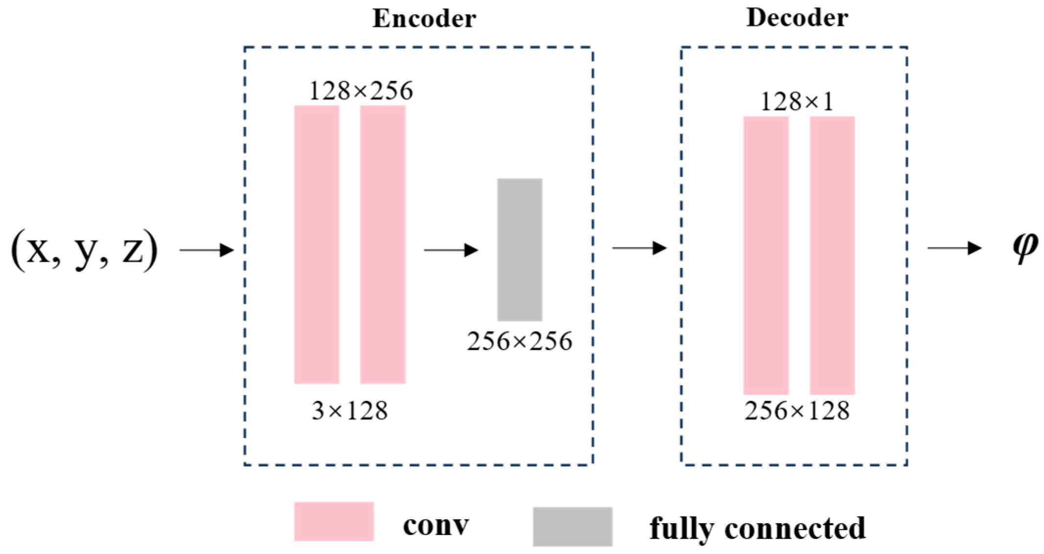
Auto-Encoder (AE) Model	Pre-training Stage	L1, L2 loss function	Encoder: Conv(3 × 128) → Conv(128 × 256) → FC(256 × 256) Decoder: Conv(256 × 128) → Conv(128 × 1)	Construct the Basic Model Structures of SAE and GeoSAE
Stacked Auto-Encoder (SAE) Model	/	/	AEF°AEF−1°⋯°AE2°AE1, “°” represents the stacking operation between model	Stack AE for a specified number of times to obtain the result
GeoSAE Method	Training and Prediction Stage	Loss Function with Geological Constraints Proposed in Section 2.1	Stack SAE for the number of specified scalar fields	The loss function is modified based on SAE to the geological constraint loss function proposed in Section 2.1, thus obtaining the GeoSAE method

.

3. Experimental Verification and Results

This approach presents a three-dimensional geological model for the Jiangdong new district in Haikou city, China, covering an area of approximately 60 square kilometers. Multiple geological constraints, including stratigraphic sequence relationships, interface consistency, attitude of production points, and smoothness of stratigraphic interfaces, are incorporated into the model. The construction of a reliable and accurate geological model is ensured by these constraints. Additionally, the impact of stratigraphic sampling points on the fitting of stratigraphic surfaces is evaluated, and the effectiveness of the stratigraphic interface smoothness constraints is validated. The experimental setup uses the following hardware and software configuration: the GPU is an NVIDIA GeForce RTX-3080Ti (NVIDIA Corporation, Santa Clara, CA, USA), the CPU is an Intel single-core i7-10 (Intel Corporation, Santa Clara, CA, USA), the CUDA version is 11.6, and the Python version is 3.8.

3.1. Data Preparation and Analysis

Haikou Jiangdong new district is situated in the northeastern region of Hainan Island, with coordinates ranging from 110°22′ to 110°38′ east longitude and 19°53′ to 20°04′ north latitude. The study area extends from Wenchang city to Nandujiang river in the east–west direction, covering approximately 298 square kilometers, and reaches from Yunlong town to Qiongzhou strait in the north–south direction. The study area covers about 298 square kilometers, extending east–west from Wenchang city to the Nandu river, and north–south from Yunlong town to the Qiongzhou strait. The area features diverse and complex landforms, which can be classified into volcanic, fluvial, and marine types based on their origin. Volcanic landforms are primarily found in the south-central region of Jiangdong new district and near Yanfeng town. Fluvial landforms are concentrated in the southwestern part of Lingshan town, while marine landforms are widespread in the northern Guilin Yang area [36,37].

The regional stratigraphy of the study area is characterized by Carboniferous to Permian gneiss and mixed rocks as the underlying bedrock. Overlying these, from oldest to youngest, are the Miocene Dengloujiao Formation, Pliocene Haikou Formation, Pleistocene Xiuying Formation, Beihai Formation, Duowen Formation, and Holocene formations such as the Qiongshan and Yandun Formations. Additionally, there are broken alluvial deposits (Qh). These strata are distributed within a depth of approximately 100 m [38,39]. Due to differences in their formation periods and depositional environments, these strata exhibit significant variations in their engineering geological properties. Therefore, the stratigraphic contact relationships must be organized based on actual field investigation and drilling data from the Jiangdong new district, as outlined in

Table 2. Standard stratigraphic sequences and contact relationships of Neoproterozoic–Quaternary in Jiangdong new district, Haikou city, at a depth of approximately 100 m.

Geological Age System				Formation Group	Sedimentary Environment	Stratigraphic Code	Contact (to Upper Strata)
Era	Period	Epoch	Age
Cenozoic	Quaternary system	Holocene epoch	undivided	Alluvial deposits Qh	fluvial facies	1-1-1	/
			upper	Yandun group Qh3y	coastal-lagoon facies	1-1-2	parallel unconformable
			middle	Qiongshan group Qh2q	deltaic facies	1-1-3	conformable
		Pleistocene epoch	middle	Duowen Group Qp2d	volcanic facies	1-2-1	parallel unconformable
				Beihai group Qp2b	alluvial fan facies	1-2-2	parallel unconformable
			lower	Xiuying group Qp1x	lacustrine facies	1-2-3	parallel unconformable
	Neogene series	Pliocene epoch		Haikou groupN2h	shallow marine shelf/barrier island facies	2-1-1	parallel unconformable
		Miocene epoch		Dengjiaolou Group N1d	shallow marine shelf facies	2-2-1	conformable

.

The method presented in this paper primarily focuses on simulation modeling of unconformities. In the study area, boreholes primarily represent Quaternary and Neoproterozoic strata, with some areas exhibiting missing or sparse stratigraphic data. To minimize the impact of sparse borehole distribution and other data quality issues on method validation, the borehole data were cleaned and supplemented, and virtual boreholes were added. This process resulted in the creation of the geological dataset used for the experiments. A total of 517 boreholes from the Jiangdong new district of Haikou city were included, with the specific borehole distribution and modeling area shown in Figure 9.

The stratigraphic column derived from the stratigraphic contact relationships is shown in Figure 10, and the corresponding potential fields, constructed based on the stratigraphic sequence relationships for each surface, are detailed in

Table 3. Construction of potential fields and stratigraphic relationships between stratigraphic surfaces in the modeled area.

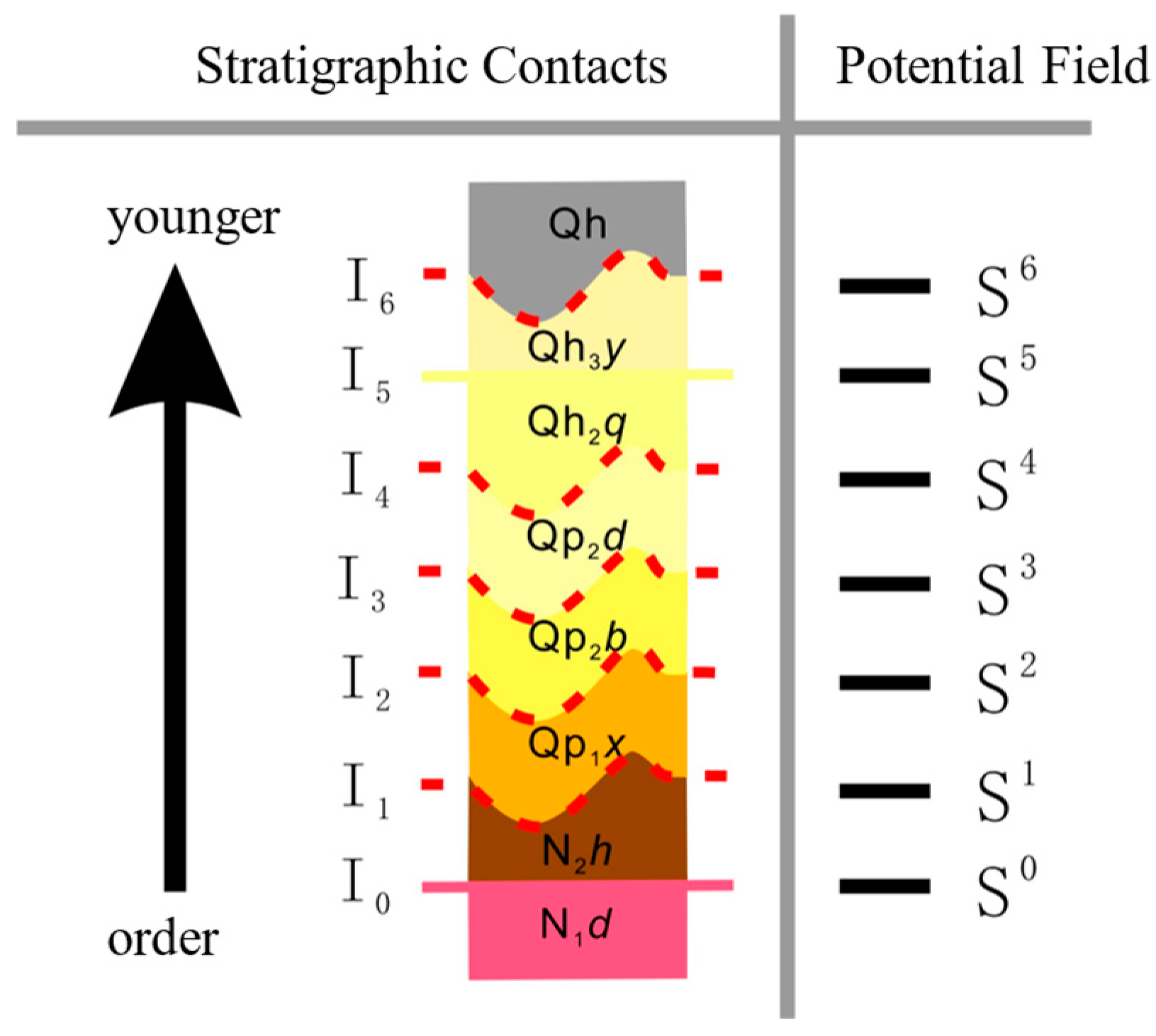
Stratigraphic Surfaces	Formation Group	Stratigraphic Code	Potential Field Code	Upper Geological Interface	Lower Geological Interface
I0	N1d	2-2-1	S0	None	None
I1	N2h	2-1-1	S1	None	I0
I2	Qp1x	1-2-3	S2	None	I0, I1
I3	Qp2b	1-2-2	S3	None	I0, I1, I2
I4	Qp2d	1-2-1	S4	None	I0, I1, I2, I3
I5	Qh2q	1-1-3	S5	None	I0, I1, I2, I3, I4
I6	Qh3y	1-1-2	S6	None	I0, I1, I2, I3, I4, I5

. For the unintegrated surfaces, a separate potential field is constructed for each prediction. Observations indicate that there is no continuous, integrated stratigraphic surface. Consequently, individual potential fields are constructed for each stratigraphic surface, with no overlying relationships considered.

The data from 517 boreholes were discretized to obtain stratigraphic surface sampling points. Each sampling point consists of the x and y coordinates of each borehole, the top surface of each stratigraphic layer, and the corresponding stratigraphic surface code. After discretization, a total of 3619 stratigraphic surface sampling points were generated for model training. The distribution of these points is detailed in Figure 11.

3.2. Construction of Three-Dimensional Geological Models

The stratigraphic surface sampling points, with coordinates normalized to the range [−1, 1], are entered into the constructed stacked autoencoder to predict the potential field values. Section 2.1 provides a comprehensive introduction to the stacked autoencoder model used for 3D geological modeling.

The stacked autoencoder model used in this study is defined by several key parameters. The batch size is set to 128 samples per iteration, with an initial learning rate of 0.001, which is halved every 500 iterations. Pre-training is performed using planar geometry, as shown in Figure 7, and after 5000 iterations, the network parameters are loaded into each autoencoder. The model incorporates various loss functions, including stratigraphic sequence relationship loss, global smoothing loss, stratigraphic surface potential field bias, variance, and polarity-related losses. A parameterized Softplus function is used as the activation function, and the weight (λ) for the global smoothing loss is set to 0.1.

After 5000 iterations, when the training reaches convergence, the values of each loss function are presented in

Table 4. Details of each loss function for 3D stratigraphic surface modeling of stratigraphic points in Jiangdong new district.

Model Loss Metrics	Worth
Loss of stratigraphic consistency	0.00336
Global smoothing loss	0.02705
Potential field bias loss	0.05635
Potential field variance loss	0.00114

. The stratigraphic consistency loss measures how well the model-generated stratigraphic surfaces align with the geological sequence. A low value indicates that the model accurately reflects the stratigraphic distribution, maintaining continuity and relative positioning of the surfaces. The global smoothing loss evaluates the model’s spatial smoothness, aiming to prevent abrupt or unnatural changes in the stratigraphic surfaces. A low value suggests that the model maintains smooth transitions throughout and avoids excessive local fluctuations. The potential field deviation loss quantifies the difference between the predicted and actual potential fields. A slightly higher value indicates that the model may underperform in some regions, requiring further optimization to reduce discrepancies with real data. The potential field variance loss measures the variability in the predicted potential field, reflecting the stability and consistency of the model. A very small value suggests that the model is stable across most areas, with high consistency in its predictions.

The 3D potential field is shown in Figure 12, with isosurface extraction performed using the PyVista open-source library [40]. The resulting 3D stratigraphic surface model is displayed in Figure 13. The model’s spatial resolution is 50 m in the x and y directions and 10 m in the z direction, enabling detailed capture of stratigraphic variations and ensuring the model accurately represents the geological structure. Figure 14 presents a 3 × 3 section of the model, illustrating the fit of the data within the model.

The fit between each modeled stratigraphic surface and its corresponding sampling points is shown in Figure 15, with panels a to g representing seven strata, ordered from youngest to oldest. The modeled surfaces and the sampling points generally align well, with most points overlapping the surfaces. However, a few points lie outside the surfaces due to significant stratigraphic undulations, which make full constraint difficult. The core method for constructing geological models using the PyVista library involves extracting a series of consecutive isosurfaces from the potential field and processing them iteratively, from oldest to youngest. When processing an older stratigraphic surface, the algorithm identifies any younger unconformity surfaces above it that intersect with the current surface. This approach ensures the creation of a layered model that more accurately represents the geological structure. For instance, the voids observed in the Qh₂q and Qp₂d stratigraphic surfaces in Figure 15 reflect this phenomenon, indicating sedimentary discontinuities or erosional events in geological history. The N₁d stratigraphic surface in Figure 13 displays significant vertical folding, which may be attributed to two factors: complex tectonic movements that caused substantial vertical height changes and folding, and the intricate nature of the vertical sampling data for the N₁d surface, which may challenge the interpolation algorithm in capturing fine variations, leading to unnatural folds in the stratigraphic layers. Overall, the fitting results and structural features shown in Figure 15 provide important insights for geological modeling, revealing the relationships between strata and their historical evolution, thereby enhancing the understanding of complex geological processes.

The average distance residuals and variances (in real-world distances) for each stratum were calculated using the model generated by PyVista, as shown in Figure 16. The potential field values decrease progressively from younger to older strata, in accordance with the stratigraphic sequence constraints proposed in this study. For most strata, the average distance residuals are below 1 m, except for strata N₂h and N₁d, where the values approach 1 m. This indicates that the model exhibits high spatial prediction accuracy, with the predicted stratigraphic surfaces closely matching the distribution of stratigraphic surface sampling points. However, the higher variance in the mean distances for strata N₂h and N₁d reflects greater internal variability and geological complexity in the actual data, suggesting that the model does not fully capture the unique characteristics of these strata.

3.3. Comparison and Control of Stratigraphic Smoothness

The stratigraphic smoothness constraint introduced in this study limits the gradient magnitude of the potential field, ensuring gradual changes and smooth transitions along stratigraphic interfaces. Figure 17 presents the modeling results with smoothness constraint weights of 0.1, 0.05, and 0.01, respectively. Higher weights reduce undulations, resulting in a smoother overall stratigraphic model. As shown in Figure 17, decreasing the smoothness constraint weight leads to sharper edge transitions and increased folding in region 1. In region 2, lower weights cause an unnatural stepped texture, which negatively impacts the quality of isosurface extraction. This constraint not only enhances the interpretability of the model but also improves its stability in practical applications, mitigating the effects of data noise and reducing the occurrence of unnatural features.

4. Discussion

The modeling results indicate that the GeoSAE method excels in constructing 3D geological models that incorporate multiple unconformities and continuous stratigraphic interfaces. It is particularly effective in generating scalar field values that adhere to geological principles, even when handling noisy regional datasets. Although the stratigraphic sequence relationship loss and global smoothing loss contribute incrementally to model optimization, they provide crucial support for validating the model’s effectiveness. Particularly in data-scarce areas, such as outcrop regions with limited profile data, these constraints offer significant improvements. They enable the integration of geological maps into the modeling process by sampling points within unit polygons and incorporating these points as constraints with weighting terms to guide the model toward results that better reflect geological structures.

Furthermore, the GeoSAE model effectively handles both internal and external constraints on stratigraphic relationships, demonstrating its potential to integrate new geological constraints. For example, the model automatically learns the optimal isosurface for each stratigraphic surface, thus overcoming the limitations of manually specified isosurfaces. This method is more flexible in adapting to complex geological structures, especially when modeling areas with varying or significant thickness changes. Compared to the limitations of manually specified isosurfaces in traditional methods, GeoSAE significantly enhances the expression of stratigraphic structures.

Experimental results show that the Softplus function effectively captures high-frequency details in the data while avoiding unnatural folding features when generating structures with good geological representation. The ReLU activation function typically results in sharper geometric shapes, which may be more suitable for brittle structural environments, while the smoother geometric shapes produced by the Softplus function better align with the actual features of geological structures. Experimental results show that the Softplus function effectively captures high-frequency details in the data while avoiding unnatural folding features when generating structures with good geological representation. In contrast, while the ReLU activation function generates sharper geometric shapes, in certain cases, the model’s fitting performance may be compromised, especially when higher stratigraphic smoothness is required.

However, although the GeoSAE model performs excellently in fitting most stratigraphic surfaces, some layers (such as N1d and N2h) exhibit significant fitting errors. These errors may stem from the inherent complexity of the actual geological data, such as vertical folding of strata and erosional unconformities, which make it difficult for the model to fully capture the subtle variations in the strata. Moreover, while the global smoothing constraint reduces the impact of data noise to some extent, excessive smoothing weights may suppress important geological features in the strata, leading to overly smooth stratigraphic surfaces, which could affect the model’s accuracy. Therefore, future research could further optimize the weight of the smoothing constraint to better balance the smoothness of the model with the retention of details.

Overall, the GeoSAE method provides a new and effective approach for 3D geological modeling, excelling in handling complex geological structures and large-scale regional modeling. This method not only enhances the accuracy of modeling but also improves the model’s adaptability to complex geological environments, offering important references for future geological modeling and data analysis. In future work, further optimization of constraint conditions and improving the model’s ability to capture special geological phenomena remain promising areas for in-depth research.

5. Conclusions

Three-dimensional geological modeling is essential for advancing our understanding of the formation and evolution of subsurface structures. However, incorporating geological knowledge directly into the modeling process is challenging, often leading to discrepancies between the generated 3D geological models and actual geological conditions. To address this issue, this work presents a geological constraint-driven 3D geological modeling approach, GeoSAE, which effectively integrates multiple geological constraints—such as stratigraphic sequence relationships, interface consistency, attitude point orientation, and interface smoothness—into the deep learning training process. The core contributions of this work are the construction of a geological constraint loss function that incorporates stratigraphic geometric features and smoothing effects to guide the training process; the design of a stacked autoencoder (SAE) structure that enables the simultaneous prediction of multiple potential field values; and the development of a comprehensive framework for geological constraint-driven 3D geological modeling, which is validated through modeling experiments.

The proposed method utilizes a deep learning approach with integrated geological constraints, overcoming the limitations of traditional implicit interpolation techniques. The experimental results show that GeoSAE accurately predicts stratigraphic surfaces and fits stratigraphic points with high precision. Additionally, the stratigraphic smoothness constraint effectively mitigates abrupt transitions in potential field modeling, enhancing the quality of the generated model.

This method’s key advantage lies in its ability to incorporate geological constraints directly into the modeling process, improving both model accuracy and geological relevance. Future work may focus on extending the method to model more complex geological structures, such as faults and overturned strata. Additionally, incorporating more geological constraints and expanding the dataset could further refine the framework’s ability to handle complex geological challenges. Exploring more flexible network architectures and integrating multivariate geological data may also improve the model’s generalization and performance.

References

- Birch, C. New Systems for Geological Modelling-Black Box or Best Practice? J. S. Afr. Inst. Min. Metall. 2014, 114, 993–1000. [Google Scholar]
- McInerney, P.; Goldberg, A.; Calcagno, P.; Courrioux, G.; Guillen, A.; Seikel, R. Improved 3D Geology Modelling Using an Implicit Function Interpolator and Forward Modelling of Potential Field Data. In Proceedings of the Exploration 07: Fifth Decennial International Conference on Mineral Exploration, Toronto, ON, Canada, 9–12 September 2007; Volume 7, pp. 919–922. [Google Scholar]
- Wellmann, F.; Caumon, G. 3-D Structural Geological Models: Concepts, Methods, and Uncertainties. In Advances in Geophysics; Elsevier: Amsterdam, The Netherlands, 2018; Volume 59, pp. 1–121. [Google Scholar]
- Si, H. Constrained Delaunay Tetrahedral Mesh Generation and Refinement. Finite Elem. Anal. Des. 2010, 46, 33–46. [Google Scholar] [CrossRef]
- Wang, B.; Wu, L.; Li, W.; Qiu, Q.; Xie, Z.; Liu, H.; Zhou, Y. A Semi-Automatic Approach for Generating Geological Profiles by Integrating Multi-Source Data. Ore Geol. Rev. 2021, 134, 104190. [Google Scholar] [CrossRef]
- Lyu, M.; Ren, B.; Wu, B.; Tong, D.; Ge, S.; Han, S. A Parametric 3D Geological Modeling Method Considering Stratigraphic Interface Topology Optimization and Coding Expert Knowledge. Eng. Geol. 2021, 293, 106300. [Google Scholar] [CrossRef]
- Gonçalves, Í.G.; Kumaira, S.; Guadagnin, F. A Machine Learning Approach to the Potential-Field Method for Implicit Modeling of Geological Structures. Comput. Geosci. 2017, 103, 173–182. [Google Scholar] [CrossRef]
- González-Garcia, J.; Jessell, M. A 3D Geological Model for the Ruiz-Tolima Volcanic Massif (Colombia): Assessment of Geological Uncertainty Using a Stochastic AResearch on 3D Geological Modelingpproach Based on Bézier Curve Design. Tectonophysics 2016, 687, 139–157. [Google Scholar] [CrossRef]
- De Kemp, E.A.; Sprague, K.B. Interpretive Tools for 3-D Structural Geological Modeling Part I: Bezier-Based Curves, Ribbons and Grip Frames. GeoInformatica 2003, 7, 55–71. [Google Scholar] [CrossRef]
- Mallet, J.-L. Discrete Smooth Interpolation in Geometric Modelling. Comput.-Aided Des. 1992, 24, 178–191. [Google Scholar] [CrossRef]
- Mallet, J.-L. Discrete Smooth Interpolation. ACM Trans. Graph. 1989, 8, 121–144. [Google Scholar] [CrossRef]
- Collon, P.; Steckiewicz-Laurent, W.; Pellerin, J.; Laurent, G.; Caumon, G.; Reichart, G.; Vaute, L. 3D Geomodelling Combining Implicit Surfaces and Voronoi-Based Remeshing: A Case Study in the Lorraine Coal Basin (France). Comput. Geosci. 2015, 77, 29–43. [Google Scholar] [CrossRef]
- Zhong, D.; Wang, L.; Lin, B.I.; Jia, M. Implicit Modeling of Complex Orebody with Constraints of Geological Rules. Trans. Nonferrous Met. Soc. China 2019, 29, 2392–2399. [Google Scholar] [CrossRef]
- de la Varga, M.; Schaaf, A.; Wellmann, F. GemPy 1.0: Open-Source Stochastic Geological Modeling and Inversion. Geosci. Model Dev. 2019, 12, 1–32. [Google Scholar] [CrossRef]
- Marinoni, O. Improving Geological Models Using a Combined Ordinary–Indicator Kriging Approach. Eng. Geol. 2003, 69, 37–45. [Google Scholar] [CrossRef]
- Frank, T.; Tertois, A.-L.; Mallet, J.-L. 3D-Reconstruction of Complex Geological Interfaces from Irregularly Distributed and Noisy Point Data. Comput. Geosci. 2007, 33, 932–943. [Google Scholar] [CrossRef]
- Cuomo, S.; Galletti, A.; Giunta, G.; Marcellino, L. Reconstruction of Implicit Curves and Surfaces via RBF Interpolation. Appl. Numer. Math. 2017, 116, 157–171. [Google Scholar] [CrossRef]
- Skala, V. RBF Interpolation with CSRBF of Large Data Sets. Procedia Comput. Sci. 2017, 108, 2433–2437. [Google Scholar] [CrossRef]
- Wellmann, J.F.; Lindsay, M.; Poh, J.; Jessell, M. Validating 3-D Structural Models with Geological Knowledge for Improved Uncertainty Evaluations. Energy Procedia 2014, 59, 374–381. [Google Scholar] [CrossRef]
- Guo, J.; Wang, J.; Wu, L.; Liu, C.; Li, C.; Li, F.; Lin, M.; Jessell, M.W.; Li, P.; Dai, X. Explicit-Implicit-Integrated 3-D Geological Modelling Approach: A Case Study of the Xianyan Demolition Volcano (Fujian, China). Tectonophysics 2020, 795, 228648. [Google Scholar] [CrossRef]
- Ross, M.; Taylor, A.; Kelley, S.; Lopez, S.; Allanic, C.; Courrioux, G.; Bourgine, B.; Calcagno, P.; Carit, S.; Gabalda, S. Integrated Rule-Based Geomodeling—Explicit and Implicit Approaches. In Applied Multidimensional Geological Modeling; Keith Turner, A., Kessler, H., Van Der Meulen, M.J., Eds.; Wiley: Hoboken, NJ, USA, 2021; pp. 273–294. ISBN 978-1-119-16312-1. [Google Scholar]
- Liu, L.; Li, T.; Ma, C. Research on 3D Geological Modeling Method Based on Deep Neural Networks for Drilling Data. Appl. Sci. 2024, 14, 423. [Google Scholar] [CrossRef]
- Zhou, C.; Ouyang, J.; Ming, W.; Zhang, G.; Du, Z.; Liu, Z. A Stratigraphic Prediction Method Based on Machine Learning. Appl. Sci. 2019, 9, 3553. [Google Scholar] [CrossRef]
- Guo, J.; Li, Y.; Jessell, M.W.; Giraud, J.; Li, C.; Wu, L.; Li, F.; Liu, S. 3D Geological Structure Inversion from Noddy-Generated Magnetic Data Using Deep Learning Methods. Comput. Geosci. 2021, 149, 104701. [Google Scholar] [CrossRef]
- Cui, Z.; Chen, Q.; Liu, G.; Xun, L. SA-RelayGANs: A Novel Framework for the Characterization of Complex Hydrological Structures Based on GANs and Self-Attention Mechanism. Water Resour. Res. 2024, 60, e2023WR035932. [Google Scholar] [CrossRef]
- Yang, Z.; Chen, Q.; Cui, Z.; Liu, G.; Dong, S.; Tian, Y. Automatic Reconstruction Method of 3D Geological Models Based on Deep Convolutional Generative Adversarial Networks. Comput. Geosci. 2022, 26, 1135–1150. [Google Scholar] [CrossRef]
- Chen, Q.; Cui, Z.; Liu, G.; Yang, Z.; Ma, X. Deep Convolutional Generative Adversarial Networks for Modeling Complex Hydrological Structures in Monte-Carlo Simulation. J. Hydrol. 2022, 610, 127970. [Google Scholar] [CrossRef]
- Hillier, M.; Wellmann, F.; Brodaric, B.; De Kemp, E.; Schetselaar, E. Three-Dimensional Structural Geological Modeling Using Graph Neural Networks. Math. Geosci. 2021, 53, 1725–1749. [Google Scholar] [CrossRef]
- Giraud, J.; Caumon, G.; Grose, L.; Ogarko, V.; Cupillard, P. Integration of Automatic Implicit Geological Modelling in Deterministic Geophysical Inversion. Solid Earth 2024, 15, 63–89. [Google Scholar] [CrossRef]
- Bi, Z.; Wu, X.; Geng, Z.; Li, H. Deep Relative Geologic Time: A Deep Learning Method for Simultaneously Interpreting 3-D Seismic Horizons and Faults. J. Geophys. Res. Solid Earth 2021, 126, e2021JB021882. [Google Scholar] [CrossRef]
- Hillier, M.; Wellmann, F.; de Kemp, E.A.; Brodaric, B.; Schetselaar, E.; Bédard, K. GeoINR 1.0: An Implicit Neural Network Approach to Three-Dimensional Geological Modelling. Geosci. Model Dev. 2023, 16, 6987–7012. [Google Scholar] [CrossRef]
- Pan, D.; Xu, Z.; Lu, X.; Zhou, L.; Li, H. 3D Scene and Geological Modeling Using Integrated Multi-Source Spatial Data: Methodology, Challenges, and Suggestions. Tunn. Undergr. Space Technol. 2020, 100, 103393. [Google Scholar] [CrossRef]
- Charte, D.; Charte, F.; del Jesus, M.J.; Herrera, F. An Analysis on the Use of Autoencoders for Representation Learning: Fundamentals, Learning Task Case Studies, Explainability and Challenges. Neurocomputing 2020, 404, 93–107. [Google Scholar] [CrossRef]
- Aster, R.C.; Thurber, C.H.; Borchers, B. Parameter Estimation and Inverse Problems; Elsevier: Amsterdam, The Netherlands, 2012. [Google Scholar]
- Gropp, A.; Yariv, L.; Haim, N.; Atzmon, M.; Lipman, Y. Implicit Geometric Regularization for Learning Shapes. arXiv 2020, arXiv:2002.10099. [Google Scholar]
- Liu, L.; Zhou, J.; Jiang, D.; Zhuang, D.; Mansaray, L.R. Lithological Discrimination of the Mafic-Ultramafic Complex, Huitongshan, Beishan, China: Using ASTER Data. J. Earth Sci. 2014, 25, 529–536. [Google Scholar] [CrossRef]
- Su, Q.; Li, Z.; Li, G.; Zhu, D.; Hu, P. Coastal Erosion Risk Assessment of Hainan Island, China. Acta Oceanol. Sin. 2023, 42, 79–90. [Google Scholar] [CrossRef]
- Dilek, Y.; Tang, L. Magmatic Record of the Mesozoic Geology of Hainan Island and Its Implications for the Mesozoic Tectonomagmatic Evolution of SE China: Effects of Slab Geometry and Dynamics in Continental Tectonics. Geol. Mag. 2021, 158, 118–142. [Google Scholar] [CrossRef]
- Yao, W.; Li, Z.X.; Li, W.X.; Li, X.H. Proterozoic Tectonics of Hainan Island in Supercontinent Cycles: New Insights from Geochronological and Isotopic Results. Precambrian Res. 2017, 290, 86–100. [Google Scholar] [CrossRef]
- Sullivan, C.; Kaszynski, A. PyVista: 3D Plotting and Mesh Analysis through a Streamlined Interface for the Visualization Toolkit (VTK). J. Open Source Softw. 2019, 4, 1450. [Google Scholar] [CrossRef]