Photovoltaic Power Plants with Horizontal Single-Axis Trackers: Influence of the Movement Limit on Incident Solar Irradiance

Abstract

This paper presents an energy analysis of the influence of the movement limit of a horizontal single-axis tracker on the incident energy on the photovoltaic field. The procedure used comprises the following steps: (i) the determination of the periods of operation of a horizontal single-axis tracking; (ii) the analytical determination of the annual, daily, and hourly incident solar irradiance on the photovoltaic field; (iii) the validation of the model; and (iv) the definition of the evaluation indicators. The study focused on three photovoltaic power plants in Spain (Miraflores $PV$ power plant, Basir $PV$ power plant, and Canredondo $PV$ power plant). Four evaluation indicators (annual energy loss, daily energy loss, beam component, and diffuse component) and ten movement limits, ranging from $\pm 50$ (°) to $\pm 60$ (°), were analysed. In Spain, photovoltaic power plants usually have a movement limit of $\pm 60$ (°), which is why it has been called the current scenario. According to this study, the following conclusions can be drawn: (i) It is necessary to calculate the optimal movement limit for each site under study at the design stage of the PV power plant. Although the energy loss per square metre for not using the optimal boundary movement is small, due to the large surface of the photovoltaic field, these energy losses cannot be neglected. For example, in the Canredondo photovoltaic power plant, the limit movement is not optimised and the annual energy loss is 18.49 (MWh). (ii) The higher the range of the limiting movement, the shorter the duration of the static operating period. Therefore, when the current scenario starts the normal tracking mode (where the beam component is maximised), the other scenarios remain in the static mode of operation in a horizontal position, which impairs the incidence of the beam component and favours the diffuse component. (iii) The type of day, in terms of cloudiness index, prevailing at a given location affects the choice of the movement limit. If the beam component is predominant, it favours the performance of the current scenario. In contrast, if the diffuse component is predominant, it favours scenarios other than the current scenario.

1. Introduction

Electric power is key in modern societies as it is present in many aspects of daily life. Therefore, global electricity demand increased by $2.2\%$ in 2023 [1]. Furthermore, with the expansion of hydrogen production and electric vehicles, this dependence will grow further. Figure 1 shows the global electricity demand in very important applications, as follows [2]: (i) hydrogen production, (ii) energy-intensive industries (steel, chemical, non-metallic minerals, non-ferrous metals, paper industries, etc.), (iii) other industries (construction, mining, textile, etc.), (iv) household appliances and cooking (cookers, ovens, refrigerators, washing machines, dishwashers, clothes dryers, computers, televisions, etc.), (v) cooling and heating (space heating, water heating, and space cooling in buildings), and (vi) light-duty vehicles. This global electricity demand is at the centre of the 2022 and estimated 2050 scenarios. The estimated increase in electricity demand in 2050 compared to 2022 is as follows: (i) $39.43\%$ for hydrogen production, (ii) $22.17\%$ for energy-intensive industries, (iii) $20.23\%$ for other industries, (iv) $13.83\%$ for household appliances and cooking, (v) $15.31\%$ for cooling and heating, and (vi) $18.97\%$ for light-duty vehicles.

Figure 1. World electricity demand vs. applications, 2022–2050.

Electricity generation to meet this high demand is currently the largest source of carbon dioxide (CO²) emissions in the world [1]. Global CO² emissions from electricity generation increased by $1\%$ in 2023 [1]. The use of coal in electricity generation was responsible for this increase in CO² emissions from the global power sector. These high CO² emissions have put this issue at the top of the political agenda in many countries. At the same time, the electricity sector is leading the transition towards the decarbonisation of strategic sectors, with the aim of achieving net-zero emissions in this sector. In 2023, the use of fossil fuels in power generation was $61\%$ globally [1]. This is estimated to drop to $54\%$ in 2026 [1]. To this end, it has promoted the use of renewable energies such as solar and wind power.

The European Union promotes environmental regulations for the decarbonisation of the electricity sector [3]. These regulations encourage the use of renewable energy sources in electricity generation. Wind and solar energy are two clear examples of clean and sustainable energy sources that can meet the demand for electricity.

The availability of solar energy worldwide makes solar photovoltaic ($PV$) technology a reliable solution used to reduce CO² emissions from the electricity sector and to comply with the environmental constraints in many countries. This technology is particularly attractive due to the following characteristics: (i) ease of installation, (ii) low maintenance, and (iii) scalability.

The choice of a mounting system for $PV$ modules in the design phase of a $PV$ power plant is based on maximising the power generation, reliability, durability, and maintenance efficiency of the system [4]. It is not possible to maximise all four objectives at the same time.

$PV$ module mounting systems can be implemented depending on the movements around a given axis as follows [5]: (i) dual-axis trackers, and (ii) single-axis trackers. Comparing these two systems, it can be concluded that dual-axis tracking systems generate more electrical power [6], although maintenance costs are higher [7], and they also have lower reliability and durability [4]. These characteristics are the reason for prioritising the use of horizontal single-axis trackers in $PV$ plants [4]. Horizontal single-axis trackers are estimated to have a market share of more than $95\%$ [8], as they are cheap, easy to install, and have minimal operating costs. These advantages are reflected in the global solar tracker market [4]. In 2022, this market was valued at $USD$ $3.2$ billion, and it is estimated to reach $USD$ $7.2$ billion by 2033 [4]. Therefore, this study focuses on this $PV$ module mounting system.

The operation modes of a horizontal single-axis tracker are defined to track the daily movement of the Sun and to avoid shadowing between adjacent solar trackers. There are three modes of operation as follows [9]: (i) backtracking mode, (ii) static mode, and (iii) normal tracking mode.

Avoiding shading between adjacent solar trackers is one of the most important premises in the design of a $PV$ power plant. Sunrise and sunset, characterised by low solar elevations, are the critical periods from this point of view. Backtracking algorithms are used to avoid shading during these periods. These algorithms determine the tilt angle of the $PV$ field that avoids shadows on adjacent solar trackers and also maximises the incident beam solar irradiance. This period of operation is called the backtracking mode.

The operation static mode is characterised by the limit of movement ($\pm {\beta }_{max}$) of the $PV$ field. Thus, if the position of the Sun defines the $PV$ field arrangement with a tilt angle greater than the movement limit to obtain the maximum incident beam solar irradiance, the tracking algorithm will set the tilt angle to ${\beta }_{max}$.

The normal tracking mode is the longest period of operation of the solar tracker. In this mode, the tracking algorithm places the $PV$ field in the position that maximises the incident beam solar irradiance by maximising the cosine of the solar incidence angle [10].

Once the $PV$ module mounting system has been chosen, the next step is to determine a number of parameters that define the design of a $PV$ power plant. These parameters are the following [9]: the shape of the available land, tilt angle of the terrain, the azimuth angle of solar tracker, the pitch, the configuration of $PV$ modules, the movement limit, etc. This paper analyses the influence of the movement limit of a horizontal single-axis tracker on the incident energy on the $PV$ field.

Table 1 shows several $PV$ power plants in Spain that use single-axis solar tracking technology. The vast majority of these $PV$ plants are characterised by the use of $\pm 60$ ($°$) as the limit of movement. A question arises with respect to this choice; is this movement limit suitable for all locations from the point of view of the incident solar irradiance on the $PV$ field?

Table 1. Specifications of some PV power plants located in Spain.

PV	Location	Latitude	Longitude	Altitude	Power	Movement Limit
Power Plant				(m)	(MWp)	($°$)
Basir	Cádiz	$36°{20}^{\prime }{24}^{″}$ N	$5°{50}^{\prime }32.6^{″}$ W	104	20.013	$\pm 60$
Yarte	Cadiz	$36°{36}^{\prime }21.{96}^{″}$ N	$5°{47}^{\prime }55.{68}^{″}$ W	143	50.000	$\pm 60$
Mula II	Murcia	$37°{59}^{\prime }24.{21}^{″}$ N	$1°{24}^{\prime }41.{90}^{″}$ W	313	114.400	$\pm 60$
Jumilla	Murcia	$38°{27}^{\prime }14.{48}^{″}$ N	$1°{16}^{\prime }42.{94}^{″}$ W	510	8.900	$\pm 55$
Campos	Murcia	$38°3^{\prime }42.{25}^{″}$ N	$1°{23}^{\prime }27.{23}^{″}$ W	172	109.190	$\pm 60$
Miraflores	Badajoz	$38°{46}^{\prime }4.8^{″}$ N	$5°{32}^{\prime }49.{199}^{″}$ W	1162	22.000	$\pm 60$
Plato	Madrid	$40°{22}^{\prime }18.{92}^{″}$ N	$3°{19}^{\prime }46.{99}^{″}$ W	809	22.580	$\pm 60$
Campos de Teruel	Teruel	$40°{47}^{\prime }35.{60}^{″}$ N	$2°{46}^{\prime }37.{23}^{″}$ E	1292	25.000	$\pm 60$
Canredondo	Guadalajara	$40°{47}^{\prime }58.{886}^{″}$ N	$2°{31}^{\prime }26.{95}^{″}$ W	1162	21.980	$\pm 60$

The limit of movement is a parameter that is not usually taken into account in studies related to $PV$ power plant design. There are many studies that do not consider this parameter, and other studies consider this parameter but without analysing the consequences of its variation. Several studies that corroborate this statement will be discussed below.

Some of the publications on single-axis solar trackers that take into account the limit of movement include the following:

(i)

In [11], the optimal deployment of horizontal single-axis trackers in a terrain characterised by its tilt angle and variable orientation was studied. A single movement limit of $\pm 55$ (°) was used without considering the effects of this parameter on the results of incident solar irradiance on the $PV$ field.

(ii)

López [12] analysed a real $PV$ power plant from the point of view of the tilt angle and orientation of the horizontal single-axis trackers. A movement limit of $\pm 55$ ($°$) was used without further investigation of the influence of this parameter.

(iii)

Keiner et al. [13] presented a study on backtracking strategies in horizontal single-axis trackers. The objective of the work was to choose the backtracking strategy that optimised the incident solar irradiance on the $PV$ field. This paper took into account the limit of movement, which remained constant throughout the study at a value of $\pm 50$ ($°$). Therefore, this study did not take into account the influence of the movement limit of the solar tracker on the incident solar irradiance on the $PV$ field.

(iv)

The optimisation of $PV$ power plants with horizontal single-axis trackers was the subject of the study presented in [9]. In this work, equations were presented for the calculation of the incident solar irradiance on the $PV$ field, which took into account several design parameters such as the irregular shape of the terrain, the size and configuration of the $PV$ module mounting system, the row spacing, the operating periods, and the optimal deployment of the $PV$ module mounting systems. A movement limit of $\pm 60$ ($°$) was used, but the influence of this parameter was not taken into account.

(v)

A study on tree crops between rows of horizontal single-axis trackers was presented in [14]. A movement limit of $\pm 55$ ($°$) was chosen, without analysing the influence of this factor.

(vi)

An energy analysis of the influence of the movement limit on a solar tracker was presented in [15]. In this study, only one location was analysed, so a detailed comparison of the impact of the motion limit was not performed.

On the other hand, there are a large number of studies that do not take into account the movement limit, including the following:

(i)

Anderson and Jensen [16] developed a generalised equation for horizontal single-axis trackers deployed on cross-slope terrain. By not taking into account the movement limit, the developed equation loses generality.

(ii)

Huang et al. [17] analysed the optimal tilt angle of horizontal single-axis trackers using a spatial projection model and a dynamic shadow evaluation method. This work could be completed by analysing the static mode, defined by a movement limit, and the backtracking mode.

(iii)

Alves et al. [18] optimised the design of $PV$ power plants with horizontal single-trackers using a new evaluation metric. This new assessment metric is not fully defined as it does not consider the movement limit.

(iv)

Sun et al. [19] presented a model for a horizontal single-axis tracking bracket with an adjustable tilt angle to increase incident solar irradiance regardless of the maximum movement limit.

(v)

Kamran et al. [20] presented a new $MPPT$ algorithm based on the energy valley optimiser to extract the maximum energy from solar power. This study did not take into account the movement limit and the backtracking mode.

(vi)

Tina et al. [21] presented an economic study of solar-tracking photovoltaic systems installed on the water surface. The calculation of the energy generated by the $PV$ field did not take into account the limit of movement.

It can be concluded that in the design of $PV$ power plants, the works that take into account the limit of movement only consider a certain value without delving into the effect of this parameter on the incident solar irradiance on a $PV$ field. It is also true that there are a large number of works that do not consider it.

To analyse the influence of the movement limit on the incident solar irradiance on the $PV$ field, a procedure consisting of the following steps was used: (i) the determination of the periods of operation of a horizontal single-axis tracking; (ii) the analytical determination of the annual, daily, and hourly incident solar irradiance on the photovoltaic field; (iii) the validation of the model; and (iv) the definition of the evaluation indicators.

For the analysis of the influence of the movement limit on the incident solar irradiance on the $PV$ field, the following three $PV$ power plants have been selected from Table 1: (i) the Basir $PV$ power plant, (ii) the Miraflores $PV$ power plant, and (iii) the Canredondo $PV$ power plant. The evaluation indicators that have been used to study the influence of the movement limit are the following: the annual energy loss, the daily energy loss, the beam component, and the diffuse component. A range of movement limits between $\pm 50$ ($°$) and $\pm 60$ ($°$) was investigated.

Table 1 shows that most PV power plants use a movement limit of ±60 ($°$). However, is this the optimal movement limit? In the development of this work it will be shown that this movement limit is not optimal in all locations under study. Determining the optimal movement limit is necessary to improve the performance of the PV power plant over its lifetime. To perform a detailed study on the influence of the movement limit on the incident solar irradiance in the $PV$ field, it is necessary to obtain this incident solar irradiance at hourly and daily levels. This level of detail regarding solar irradiance is not available in commercial software (PVsyst 7.2, SolarFarmer 1.5, RETScreen 8.1, etc.). Therefore, it was necessary to implement a $Mathematica$ code to calculate the hourly and daily incident solar irradiance.

The main contributions of this work are as follows:

(i)

A study of the annual energy losses due to the choice of a non-optimal horizontal single-axis tracker movement limit.

(ii)

A seasonal study of the energy losses as a function of the movement limit.

(iii)

A detailed analysis of the influence of the movement limit on the components of the incident solar irradiance on the photovoltaic field.

The remainder of the paper is organised as follows: Section 2 shows the governing equations and the assessment indicators used. Section 3 presents the results obtained at three $PV$ power plants in Spain. Finally, the main conclusions of this work are drawn in Section 4.

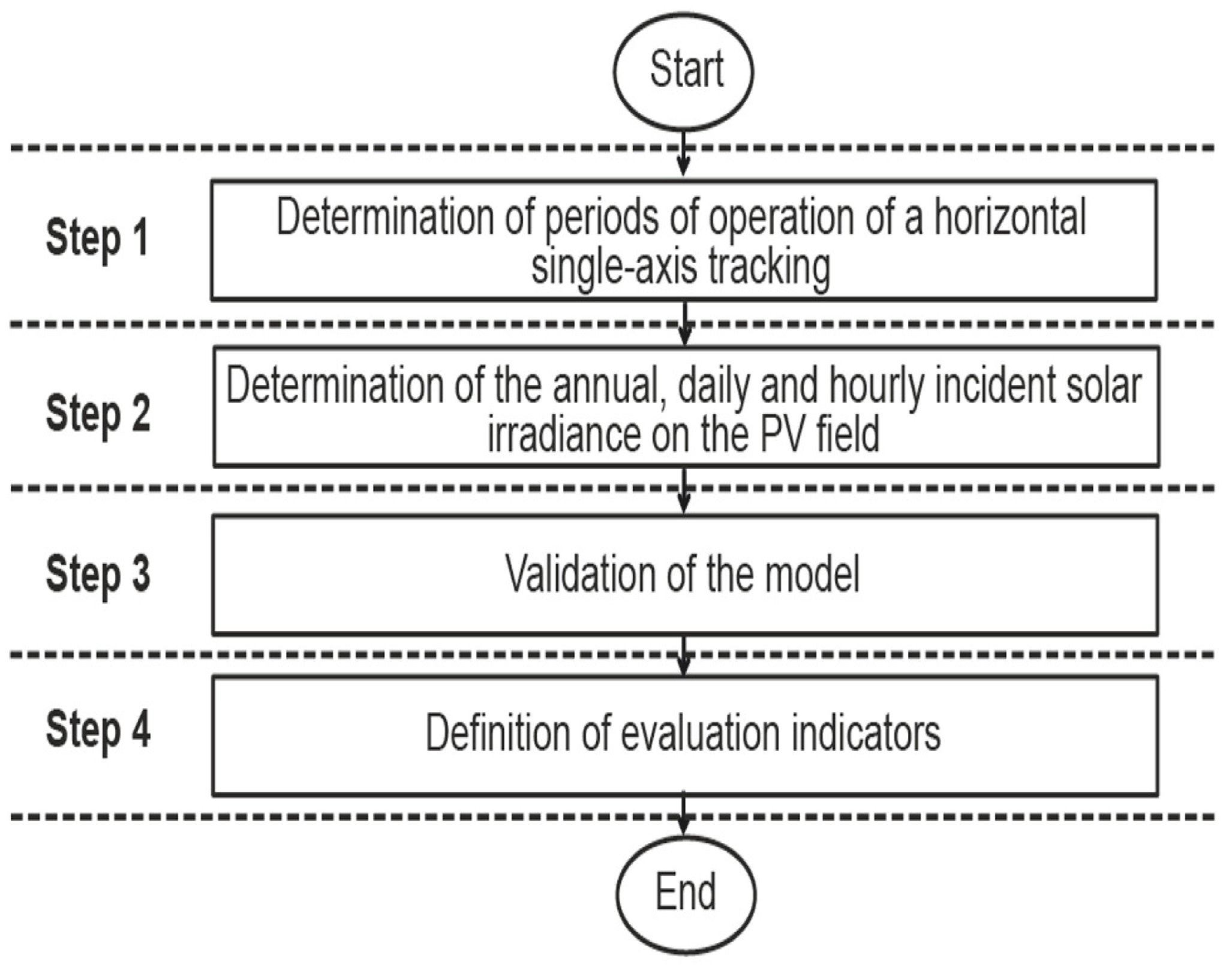
2. Materials and Methods

In general, a horizontal single-axis tracker comprises a torsion tube oriented from north to south. This tube is supported by a central column, where an electric motor is placed, and several auxiliary columns. The auxiliary columns are fitted with spherical bearings that allow rotation in the east–west direction of the $PV$ field. For mechanical reasons, this solar tracker has a movement limit, denoted by ${\beta }_{max}$. Figure 2 shows a photograph of a horizontal single-axis tracker.

Figure 2. Photograph of a horizontal single-axis tracking.

Detailed information regarding the components of the solar irradiance incident on the $PV$ field is necessary to achieve the objectives of this study. For this purpose, the procedure shown in Figure 3 was followed. This procedure consists of the following steps: (i) the determination of the periods of operation of a horizontal single-axis tracking; (ii) the determination of the annual, daily, and hourly incident solar irradiance on the $PV$ field; (iii) the validation of the model; and (iv) the definition of the evaluation indicators.

Figure 3. A flowchart describing the procedure used.

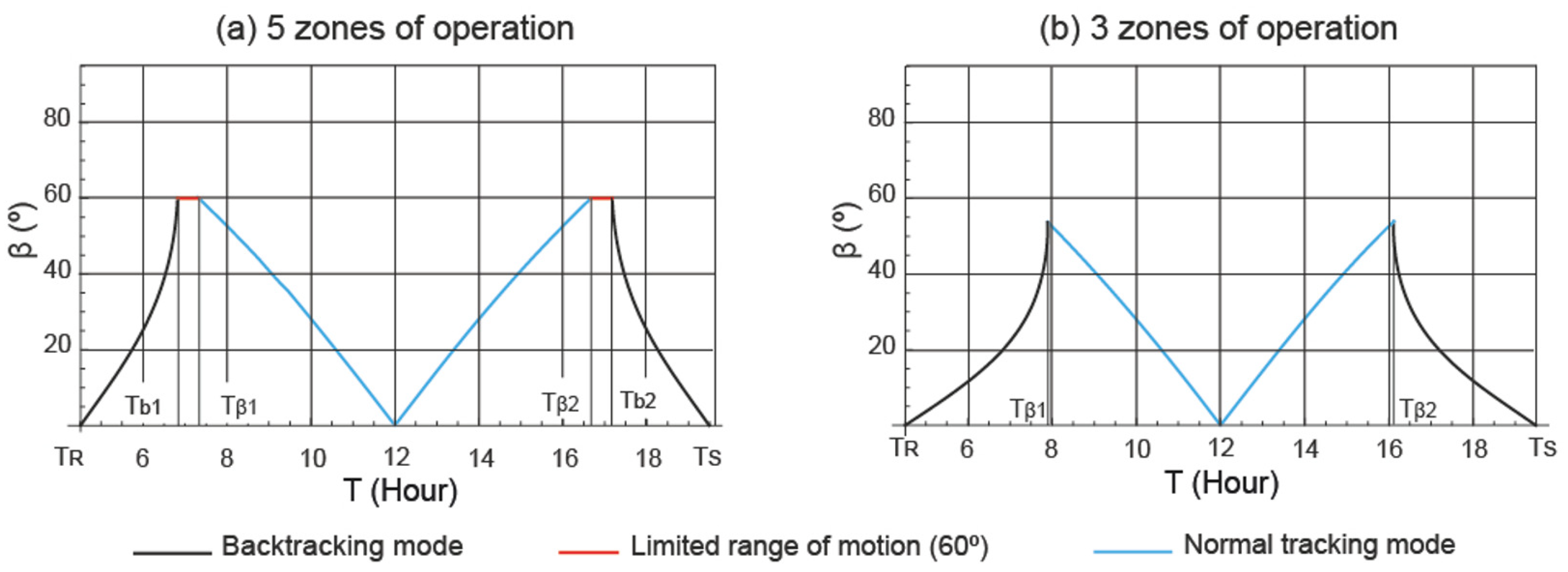
2.1. Periods of Operation of a Horizontal Single-Axis Tracking

Knowing the exact instant where the periods of operation of a horizontal single-axis tracker occur is fundamental in this study. These periods of operation are identified as follows [9]: (i) normal tracking mode, (ii) backtracking mode and (iii) static mode. Each of these operation periods has a corresponding tilt angle for the $PV$ field. These tilt angles are (i) $\beta$, (ii) ${\beta }_B$, and (iii) ${\beta }_{max}$, respectively. Obviously, these tilt angles influence the incident solar irradiance on the $PV$ field. In the following section, these angles will be determined.

The normal tracking mode is characterised by the use of a solar astronomical algorithm that allows the $PV$ field to follow the daily movement of the Sun. This period of operation lasts for most of the day. This tracking algorithm is based on maximising the solar irradiance incident on the PV field. To do this, it minimises the angle formed by the solar beam and the normal beam to the $PV$ module [10].

The backtracking mode is characterised by the use of an algorithm that avoids shadowing between adjacent solar trackers. In shaded $PV$ modules, hot spots appear that are detrimental to the $PV$ module itself [22]. The backtracking algorithm [14] is used during sunrise and sunset, when the solar height is low. This algorithm avoids shading but does not maximise the incident solar irradiance on the $PV$ field.

The static mode is characterised by the $PV$ field being stationary at the limit of movement ($\pm {\beta }_{max}$) of the solar tracker.

These three modes of operation can follow the following sequence of operation (see Figure 4a):

Figure 4. Representation of the horizontal single-axis tracker periods of operation.

(i)

Sunrise backtracking mode. This mode of operation starts at sunrise ($T_R$) and ends at the limited range of movement ($T_{b1}$). During sunrise, the position of the $PV$ field is horizontal and at the end of sunrise backtracking mode the tilt angle of the $PV$ field is ${\beta }_{max}$.

(ii)

Static mode. This mode of operation starts at the end of the sunrise backtracking mode ($T_{b1}$) and ends at the beginning of the normal tracking mode ($T_{\beta 1}$).

(iii)

Normal tracking mode. This mode of operation starts at the movement limit before noon ($T_{\beta 1}$) and ends at the movement limit after noon ($T_{\beta 2}$).

(iv)

Static mode. This mode of operation starts at the end of normal tracking mode ($T_{\beta 2}$) and ends at the beginning of the sunset backtracking mode ($T_{b2}$).

(v)

Sunset backtracking mode. This mode of operation starts at the limited range of movement ($T_{b2}$) and ends at sunset ($T_S$). During the beginning of the sunset backtracking mode, the tilt angle of the $PV$ field is ${\beta }_{max}$, and at sunset the position of the $PV$ field, the tilt angle is horizontal.

There are five zones of operation. This sequence of operation may not be repeated every day. That is, the backtracking mode ends without reaching the static mode. Therefore, it goes directly to the normal tracking mode (see Figure 4b). In the three-zone operation sequence the $PV$ field does not reach the movement limit. In this case, there is no static mode.

2.2. Incident Solar Irradiance on the Photovoltaic Field

From Figure 4, it can be deduced that it is important to independently know each of the components (beam component ($I_{bt}$), diffuse component ($I_{dt}$), and ground-reflected component ($I_{rt}$)) that make up the solar irradiance incident on the $PV$ field. In the following section, each of these components will be analysed.

2.2.1. Beam Component Modelling

The beam component is determined by the geometric relationship between the horizontal surface and the $PV$ field surface. Equation (1) is used to calculate this component as follows [10]:

$$I_{bt}\left(n,T,\beta ,\gamma \right)=I_{bh}\left(n,T\right)·{\displaystyle \frac{cos{\theta }_i}{cos{\theta }_z}}$$

(1)

where $I_{bt}\left(n,T,\beta ,\gamma \right)$ is the beam component (W/m²), $I_{bh}\left(n,T\right)$ is the horizontal beam solar irradiance (W/m²), n is the ordinal of the day (day), T is the solar time (h), $\beta$ is the tilt angle of the $PV$ field ($°$), $\gamma$ is the azimuth angle of the $PV$ field ($°$), ${\theta }_z$ is the zenith angle of the Sun ($°$), and ${\theta }_i$ is the incident angle ($°$).

2.2.2. Diffuse Component Modelling

The diffuse component is difficult to determine accurately. There are several models that can be used to calculate it. In this study, the Liu–Jordan model will be used. Equation (2) is used to calculate this component as follows [10]:

$$I_{dt}\left(n,T,\beta \right)=I_{dh}\left(n,T\right)·\left({\displaystyle \frac{1+cos\beta }{2}}\right)$$

(2)

where $I_{dt}\left(n,T,\beta ,\gamma \right)$ is the diffuse component (W/m²), $I_{dh}\left(n,T\right)$ is the horizontal diffuse solar irradiance (W/m²), n is the ordinal of the day (day), T is the solar time (h), and $\beta$ is the tilt angle of the $PV$ field ($°$).

2.2.3. Ground-Reflected Component Modelling

The ground-reflected component depends on many factors that make it impossible to calculate it accurately. Most authors use the Liu–Jordan model. Equation (3) is used to calculate this component as follows [10]:

$$I_{rt}\left(n,T,\beta \right)=(I_{bh}\left(n,T\right)+I_{dh}\left(n,T\right))·{\rho }_g·\left({\displaystyle \frac{1-cos\beta }{2}}\right)$$

(3)

where $I_{rt}\left(n,T,\beta \right)$ is the ground-reflected component (W/m²), $I_{bh}\left(n,T\right)$ is the horizontal beam solar irradiance (W/m²), $I_{dh}\left(n,T\right)$ is the horizontal diffuse solar irradiance (W/m²), ${\rho }_g$ is the ground reflectance (), n is the ordinal of the day (day), T is the solar time (h), and $\beta$ is the tilt angle of $PV$ field ($°$).

Equations (1)–(3) have been used in many studies across different locations around the world. For example, López et al. [23] used these equations in Spain, Makhdoomi and Askarzadeh [24] in Iran, Zhu et al. [25] in China, Farahat et al. [26] in Saudi Arabia, etc.

Therefore, the incident solar irradiance on the $PV$ field can be determined by Equation (4) as follows:

$$\begin{array}{c}{I}_t\left(n,T,\beta ,\gamma \right)=I_{bh}\left(n,T\right)·{\displaystyle \frac{cos{\theta }_i}{cos{\theta }_z}}+I_{dh}\left(n,T\right)·\left({\displaystyle \frac{1+cos\beta }{2}}\right)+\hfill \\ \hspace{1em}\hspace{1em}\hspace{1em}\hspace{1em}\hspace{1em}\hspace{1em}\hspace{1em}\hspace{1em}\hspace{1em}\hspace{1em}\hspace{1em}\hspace{1em}\hspace{1em}\hspace{1em}\hspace{1em}\hspace{1em}\left(I_{bh}\left(n,T\right)+I_{dh}\left(n,T\right)\right)·{\rho }_g·\left({\displaystyle \frac{1-cos\beta }{2}}\right)\hfill \end{array}$$

(4)

To calculate the three components it is necessary to know the following parameters in each mode of operation: $\beta$, $cos{\theta }_i$, $I_{bh}$ and $I_{dh}$. The considerations listed below allow Equation (4) to be used as follows:

(i)

$\beta$ parameter. The equations for determining this parameter in each mode of operation are as follows:

Equation (5) defines the position of the $PV$ field in normal tracking mode as follows [10]:

$$\beta ={\theta }_t=arctan(tan{\theta }_z\left|sin{\gamma }_s\right|)$$

(5)

where ${\theta }_t$ is the solar transversal angle ($°$), ${\theta }_z$ is the zenith angle of the Sun ($°$), and ${\gamma }_s$ is the azimuth of the Sun ($°$).

Equation (6) defines the position of the $PV$ field in backtracking mode as follows [9]:

$${\beta }_B={\theta }_t-arccos\left({\displaystyle \frac{e_t}{W}}cos{\theta }_t\right)$$

(6)

where ${\theta }_t$ is the solar transversal angle ($°$), $e_t$ is the pich (m), and W is the width of a mounting system (m).

Equation (7) defines the position of the $PV$ field in static mode as follows [9]:

$${\beta }_s=\pm {\beta }_{max}$$

(7)

(ii)

$cos{\theta }_i$ parameter. The equations for determining this parameter in each mode of operation are as follows:

Equation (8) defines the $cos{\theta }_i$ in normal tracking mode as follows [10]:

$$cos{\theta }_i=\sqrt{{cos}^2{\theta }_z+{cos}^2\delta {sin}^2\omega }$$

(8)

where $\delta$ is the solar declination ($°$), and $\omega$ is the hour angle ($°$).

Equation (9) defines the $cos{\theta }_i$ in backtracking mode as follows [9]:

$$cos{\theta }_i=cos{\beta }_{B}cos{\theta }_z+sin{\beta }_{B}sin{\theta }_{z}cos\left({\gamma }_s-\gamma \right)$$

(9)

Equation (10) defines the position of the $PV$ field in static mode as follows [9]:

$$cos{\theta }_i=cos{\beta }_{max}cos{\theta }_z+sin{\beta }_{max}sin{\theta }_{z}cos\left({\gamma }_s-\gamma \right)$$

(10)

(iii)

$I_{bh}$ and $I_{dh}$ parameters. To calculate the three components of the incident solar irradiance on the $PV$ field, it is necessary to determine the incident solar irradiance on a horizontal surface, i.e., $I_{bh}$ and $I_{dh}$. The incident solar irradiance on a horizontal surface is site-specific, as it is significantly influenced by the local distribution of cloud cover [27]. The ideal situation for calculating $I_{bh}$ and $I_{dh}$ is to have a ground-level weather station at each location. The actual situation, however, is that the number of weather stations worldwide is very low. Evidently, it is unlikely that a weather station is close to the location under study. Therefore, it is necessary to use models for the estimation of these parameters. A large number of models can be found in the specialised literature, such as the clear sky models [25], satellite-based models [28], etc.

Due to the nature of this study, it is necessary to know the hourly distribution of the incident solar irradiance on a horizontal surface, so the procedure presented in [29] was used. This work considers the meteorological conditions of each location, and it has been used in studies on the design of PV power plants [9], the prediction of solar irradiance [30], etc.

A brief description of this procedure is given as follows [29]: (Step 1) Determination of the horizontal beam solar irradiance using the Hottel clear-sky model [10]. (Step 2) Determination of the horizontal diffuse solar irradiance using the Liu and Jordan clear-sky model [10]. (Step 3) Reduction of the values obtained in steps 1 and 2 to the meteorological conditions of the location using Fourier series. The starting data for this procedure are the monthly average of the horizontal beam and the horizontal diffuse solar irradiance. These data are obtained from the $PVGIS$ database [31] for a period of 10 years. The monthly data used were obtained from the $PVGIS$-$SARAH3$ solar irradiation database [31].

Considering the case of the five operating zones shown in Figure 4a, the incident solar irradiation on the $PV$ field ($H_t$(n)) can be calculated by Equation (11) as follows [9]:

$$\begin{array}{c}{H}_t\left(n\right)={\int }_{T_R\left(n\right)}^{T_S\left(n\right)}{I}_t(n,T,\beta )dT={\int }_{T_R\left(n\right)}^{T_{b1}\left(n\right)}{I}_t\left(n,{\beta }_B,T\right)dT+{\int }_{T_{b1}\left(n\right)}^{T_{\beta 1}\left(n\right)}{I}_t\left(n,-{\beta }_{max},T\right)dT+\hfill \\ \hfill {\int }_{T_{\beta 1}\left(n\right)}^{T_{\beta 2}\left(n\right)}{I}_t\left(n,{\theta }_t,T\right)dT+{\int }_{T_{\beta 2}\left(n\right)}^{T_{b2}\left(n\right)}{I}_t\left(n,{\beta }_{max},T\right)dT+{\int }_{T_{b2}\left(n\right)}^{T_S\left(n\right)}{I}_t\left(n,{\beta }_B,T\right)dT\end{array}$$

(11)

2.3. Model Validation

A $Mathematica$ code was implemented to determine, under site meteorological conditions, the hourly distribution of each of the components of the solar irradiance incident on the $PV$ field. Equation (4) was used for this purpose. The procedure described above [29] was used to consider the meteorological conditions at the site. The validation of the model used in the solar irradiance calculations was carried out analytically using PVsyst 7.2 software. For this purpose, one of the $PV$ power plants shown in Table 1, called the Miraflores $PV$ power plant, was modelled using PVsyst version 7.2 [32] in order to compare and validate the $Mathematica$ codes developed in this study. Equation (12) was used to compare the results obtained using the two software packages as follows:

$$AIE{C}^{\ast }={\displaystyle \frac{AI{E}_{Mathematica}^{\ast }-AI{E}_{PVSyst}^{\ast }}{AI{E}_{Mathematica}^{\ast }}}·100$$

(12)

where $AIE{C}^{\ast }$ is the comparison of the annual incident energy on the $PV$ field with a movement limit of ${\beta }_{max}^{\ast }$ ($\pm 50$ to $\pm 60$ ($°$)) (%), $AI{E}_{Mathematica}^{\ast }$ is the annual incident energy on the $PV$ field using $Mathematica$ (kWh/m²) with a movement limit of ${\beta }_{max}^{\ast }$ ($\pm 50$ to $\pm 60$ ($°$)), and $AI{E}_{PVSyst}^{\ast }$ is the annual incident energy on the $PV$ field using PVsyst software with a movement limit of ${\beta }_{max}^{\ast }$ ($\pm 50$ to $\pm 60$ ($°$)) (kWh/m²). Figure 5 shows the comparison of the results obtained using the PVsyst software and the $Mathematica$ codes developed. The results using $Mathematica$ codes are superior in all the movement limits analysed. However, this difference can be considered negligible, as the results are less than $0.9\%$. The results obtained allow us to affirm that the $Mathematica$ codes developed are suitable for application in this study. The $Mathematica$ code used allows us to obtain the hourly distribution of each component of the incident solar irradiance on the $PV$ field. In contrast, the PVSyst software does not allow us to obtain the hourly distribution.

Figure 5. Comparison of results: PVsyst software and $Mathematica$ code.

2.4. Assessment Indicators

The assessment indicators that have been used to study the influence of the movement limit are the following: the annual energy loss, the daily energy loss, the beam component, and the diffuse component.

2.4.1. Annual Energy Loss

The annual energy loss ($AEL$) parameter (kWh/m²) was used to perform the annual analysis of the influence of the movement limit. Equation (13) defines the $AEL$ as follows:

$$AEL=H_{t\ast }-H_{t60}$$

(13)

where $H_{t\ast }$ is the annual incident solar irradiation on the $PV$ field with a limit of movement of ${\beta }_{max}^{\ast }$ ($\pm 50$ to $\pm 59$ ($°$)) (kWh/m²), and $H_{t60}$ is the annual incident solar irradiation on the $PV$ field with a limit of movement of $\pm 60$ ($°$) (kWh/m²).

2.4.2. Daily Energy Loss

The daily energy loss ($DEL$) parameter (Wh/m²) was used to analyse the influence of the movement limit on the seasonal energy losses. Using Equation (14), the $DEL$ can be determined as follows:

$$DE{L}_{\ast }=H_{d\ast }-H_{d60}$$

(14)

where $H_{d\ast }$ is the daily incident solar irradiation on the $PV$ field with a movement limit of ${\beta }_{max}^{\ast }$ ($\pm 50$ to $\pm 59$ ($°$)) (Wh/m²), and $H_{d60}$ is the daily incident solar irradiation on the $PV$ field with a movement limit of $\pm 60$ ($°$) (Wh/m²).

2.4.3. Analysis of the Components of the Incident Solar Irradiance on the $PV$ Field

The predominance of the beam or diffuse component influences the choice of the movement limit of the solar tracker. The components of the incident solar irradiance in the PV field were analysed in the static operation mode. For this purpose, Equations (1) and (2) were used.

3. Results and Discussion

In this section, the influence of the movement limit of a horizontal single-axis tracker on the incident solar irradiance on the $PV$ field of three active $PV$ power plants will be analysed. Several specific codes were implemented with $Mathematica$ 11 software to calculate the hourly distribution of incident solar irradiance on the $PV$ field of a horizontal single-axis tracker for each limit of movement under study. Ten movement limits were studied, ranging from $\pm 50$ ($°$) to $\pm 60$ ($°$). The assessment indicators that have been used to study the influence of the movement limit are the following: the annual energy loss, the daily energy loss, the beam component, and the diffuse component.

3.1. PV Power Plants Under Study

For the analysis of the influence of the movement limit on the incident solar irradiance on the $PV$ field, the following three $PV$ power plants have been selected from Table 1: (i) the Miraflores $PV$ power plant, (ii) the Basir $PV$ power plant, and (iii) the Canredondo $PV$ power plant. The criteria on which this choice is based are as follows:

(i)

The selected $PV$ power plants should have different levels of horizontal global and diffuse solar irradiance, in order to analyse the influence of the ${\beta }_{max}$ on the incident solar irradiance on the $PV$ field.

(ii)

The selected $PV$ power plants should have a limit of movement equal to $\pm 60$ (°), in order to be able to compare the results obtained from other limits of movement.

The technical and geographical characteristics of the investigated $PV$ power plants are presented in Table 2.

Table 2. Specifications of the PV power plants.

Specifications	PV Power Plant
	Basir	Miraflores	Canredondo
Location	Medina Sidonia, (Spain)	Castuera, (Spain)	Canredondo, (Spain)
Latitude	$36°{20}^{\prime }{24}^{″}$ N	$38°{46}^{\prime }4.8^{″}$ N	$40°{47}^{\prime }58.{886}^{″}$ N
Longitude	$5°{50}^{\prime }32.6^{″}$ W	$5°{32}^{\prime }49.{199}^{″}$ W	$2°{31}^{\prime }26.{95}^{″}$ W
Altitude (m)	104	389	1162
Power (MWp)	20.013	22.000	21.980
PV mod. number	37,408	41,122	41,084
PV mod. model	LR5-72HBD 535 (LONGI)	LR5-72HBD 535 (LONGI)	LR5-72HBD 535 (LONGI)
PV mod. dim. (mm)	2256 × 1133	2256 × 1133	2256 × 1133
Tracking type	Horiz. single-axis tracker	Horiz. single-axis tracker	Horiz. single-axis tracker
Type of control	Astronomical algorithm	Astronomical algorithm	Astronomical algorithm
Rotation angle	${\beta }_{max}=\pm 60$ (°)	${\beta }_{max}=\pm 60$ (°)	${\beta }_{max}=\pm 60$ (°)
Configuration	1V	1V	1V
Pitch ($e_t$) (m)	6000	6500	5100
Reflectance (${\rho }_g$)	0.2	0.2	0.2

As discussed in Section 2, the meteorological conditions of the $PV$ power plants under study are a key factor in this type of work. Therefore, the procedure described in Section 2 was used for the calculation of the hourly distribution of incident solar irradiance [29]. The input data were obtained from the $PVGIS$ database [31]. Table 3 shows the horizontal solar surface irradiations at the $PV$ power plants obtained with the $PVGIS$ database [31].

Table 3. Horizontal surface solar irradiations at the locations under study obtained from the PVGIS database.

Specifications	Basir		Miraflores		Canredondo
(kWh/m2)	${\mathit{H}}_{\mathit{bh}}$	${\mathit{H}}_{\mathit{dh}}$	${\mathit{H}}_{\mathit{bh}}$	${\mathit{H}}_{\mathit{dh}}$	${\mathit{H}}_{\mathit{bh}}$	${\mathit{H}}_{\mathit{dh}}$
January	56.03	30.17	48.02	28.51	41.23	25.61
February	64.19	37.39	64.59	34.21	51.81	31.87
March	85.76	55.02	86.08	52.56	71.22	51.80
April	109.94	64.58	102.51	64.75	86.08	65.02
May	152.00	68.64	141.68	71.77	120.92	75.57
June	169.40	65.56	164.27	66.70	147.19	72.93
July	182.42	62.35	189.83	58.26	176.54	63.24
August	162.41	57.08	167.48	53.68	153.86	57.90
September	115.55	52.42	115.99	49.69	104.50	52.09
October	84.56	44.92	79.17	42.69	68.37	40.61
November	54.12	33.08	47.97	31.21	36.17	30.11
December	51.14	28.37	44.36	25.50	39.62	23.13

In this study, it was necessary to consider how the meteorological parameters of the site under study affect the choice of the movement limit. For this purpose, the meteorological factor called cloudiness index was considered. The cloudiness index ($k_d$) takes into account beam and diffuse solar irradiance, thus showing the cloudiness of the sky and/or the turbidity of the atmosphere [33]. The higher the cloudiness of the sky, the higher the $k_d$. The cloudiness index is defined as the ratio of the horizontal diffuse solar irradiance ($I_{dh}$) to the horizontal global solar irradiance ($I_{gh}$) as follows [10]:

$$k_d={\displaystyle \frac{I_{dh}}{I_{gh}}}$$

(15)

Several papers have used the cloudiness index to classify sky types as follows [34]: clear, partly cloudy, and cloudy. As will be shown below, $k_d$ influences the choice of the movement limit of a solar tracker. Figure 6 shows the $k_d$ at the locations under study obtained from the $PVGIS$-$SARAH3$ solar irradiation database. In this figure, it can be seen that the Miraflores $PV$ plant has the lowest $k_d$ and the Canredondo $PV$ plant has the highest $k_d$. The maximum and minimum values occur in the spring and summer seasons, respectively.

Figure 6. Representation of $k_{\mathrm{d}}$ at the locations under study.

It should be noted that the three selected $PV$ power plants meet the selection criteria (see Table 2 and Table 3). The three selected $PV$ power plants have a movement limit of $\pm 60$ (°), which is referred to as the actual scenario.

The data shown in Table 2 and Table 3 were used to calculate the annual incident solar irradiation on the $PV$ field for the studied movement limits. Equations (4) and (11) were used for this purpose. Table 4 shows the annual incident solar irradiation on the $PV$ field obtained at the studied locations.

Table 4. Incident solar irradiation on the PV field at the locations under study.

Movement Limit	Basir	Miraflores	Canredondo
${\mathit{\beta }}_{max}$($°$)	${\mathit{H}}_{\mathit{t}}$(kWh/m2)	${\mathit{H}}_{\mathit{t}}$(kWh/m2)	${\mathit{H}}_{\mathit{t}}$(kWh/m2)
$\pm 50$	2249.16	2219.79	2007.89
$\pm 51$	2249.88	2220.77	2008.22
$\pm 52$	2250.48	2221.62	2008.46
$\pm 53$	2250.97	2222.33	2008.63
$\pm 54$	2251.36	2222.92	2008.74
$\pm 55$	2251.66	2223.41	2008.80
$\pm 56$	2251.88	2223.79	2008.82
$\pm 57$	2252.03	2224.09	2008.80
$\pm 58$	2252.12	2224.31	2008.76
$\pm 59$	2252.16	2224.46	2008.70
$\pm 60$	2252.17	2224.55	2008.64

3.2. Annual Energy Loss

In this section, the analysis of the annual energy loss will be carried out. For this, Equation (13) will be used. The annual energy loss, for the movement limits under study, is shown in Figure 7.

Figure 7. Annual energy loss.

The following conclusions can be drawn from Figure 7:

(i)

In the three $PV$ power plants analysed, the energy loss per square metre is small, but as the surface of the $PV$ field is large, these losses cannot be neglected. The choice of a movement limit different from the optimum produces energy losses that cannot be neglected, taking into account the large surface area of the $PV$ field. The surface area of the $PV$ field at the Miraflores $PV$ power plant is 105,109.81 (m²), and at the Basir and Canredondo $PV$ power plant it is (m²) 95,616.64 and 105,012.67 (m²), respectively.

(ii)

According to Figure 7a, the use of movement limits lower than $\pm 60$(°) increases the annual energy losses. Therefore, the Miraflores $PV$ power plant uses the optimal movement limit. The annual energy loss would be $120.06$ (MWh) per year if the movement limit of this $PV$ power plant were $\pm 55$ (°).

(iii)

Based on Figure 7b, the annual energy loss increases for movement limits below $\pm 60$ (°). Therefore, the Basir $PV$ power plant uses the optimal movement limit. Using a limiting movement of $\pm 55$ (°) would result in an energy loss per year of $48.76$ (MWh).

(iv)

According to Figure 7c, the maximum annual incident solar irradiation on the $PV$ field corresponds to a movement limit of $\pm 56$ (°). Therefore, as the movement limit of the Canredondo $PV$ power plant is currently $\pm 60$ (°), the movement limit is not optimised. Therefore, the annual energy loss at this $PV$ power plant is $18.49$ (MWh).

It can be concluded that it is necessary to calculate the optimal movement limit for each location under study, as the annual losses of the incident energy are not negligible.

3.3. Daily Energy Loss

In this section, the daily analysis will be performed. For this, Equation (14) will be used, considering the $\pm 50$ (°) and $\pm 55$ (°) movement limits, to compare them with the current scenario, $\pm 60$ (°). The daily energy loss, for the limits of motion under study, is shown in Figure 8.

Figure 8. Daily energy loss.

The following conclusions can be drawn from Figure 8:

(i)

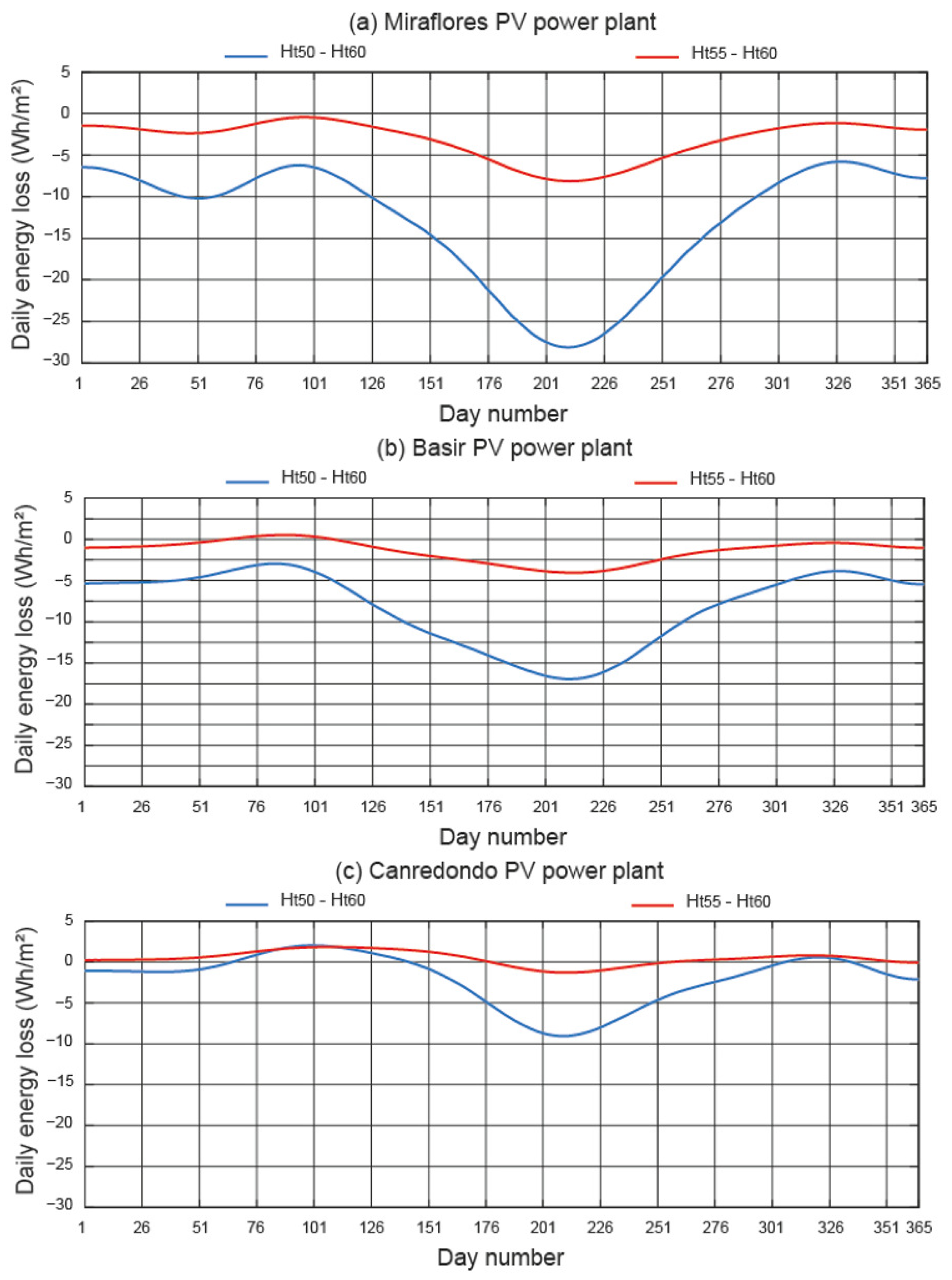
According to the red line in Figure 8a, on all days of the year, the scenario ${\beta }_{max}=\pm 55$ (°) performs worse than the current scenario. The worst results are obtained in the summer months (low $k_d$), and the best results are obtained in the spring months (high $k_d$). According to the blue line, for every day of the year too, the scenario ${\beta }_{max}=\pm 50$ (°) performs worse than the current scenario. The worst results occur in the summer months (low $k_d$). The results of the ${\beta }_{max}=\pm 50$ (°) scenario (the blue line) are worse than those of the ${\beta }_{max}=\pm 55$ (°) scenario (the red line). For example, for the day 21 March ($n=80$), the ${\beta }_{max}=\pm 60$ (°) configuration has a higher incident energy of $0.13\%$ and $0.017\%$ compared to the ${\beta }_{max}=\pm 50$ (°) and ${\beta }_{max}=\pm 55$ (°) configurations, respectively. Furthermore, for day 21 June ($n=172$), the ${\beta }_{max}=\pm 60$ (°) configuration has a higher incident energy of $0.21\%$ and $0.05\%$ compared to the ${\beta }_{max}=\pm 50$ (°) and ${\beta }_{max}=\pm 55$ (°) configurations, respectively.

(ii)

According to the red line in Figure 8b, there are very few days per year when the scenario ${\beta }_{max}=\pm 55$ (°) performs better than the current scenario. This time period corresponds to spring season (high $k_d$). Moreover, this difference is very small. In addition, the biggest difference occurs in the summer months (low $k_d$). On the other hand, according to the blue line, for every day of the year, the scenario ${\beta }_{max}=\pm 50$ (°) obtains worse results than the current scenario. The worst results occur in the summer months (low $k_d$). The results of the ${\beta }_{max}=\pm 50$ (°) scenario (the blue line) are worse than those of the ${\beta }_{max}=\pm 55$ (°) scenario (the red line). For example, for the day 21 March ($n=80$), the configuration ${\beta }_{max}=\pm 60$ (°) has an incident energy $0.05\%$ higher than the configuration ${\beta }_{max}=\pm 50$ (°) and $0.008\%$ lower than the configuration ${\beta }_{max}=\pm 55$ (°). Furthermore, for day 21 June ($n=172$), the ${\beta }_{max}=\pm 60$ (°) configuration has a higher incident energy of $0.15\%$ and $0.03\%$ compared to the ${\beta }_{max}=\pm 50$ (°) and ${\beta }_{max}=\pm 55$ (°) configurations, respectively.

(iii)

According to the red line in Figure 8c, on most days of the year, the scenario ${\beta }_{max}=\pm 55$ (°) performs better than the current scenario. The best results are obtained in the spring months (high $k_d$) and the worst results in the summer months (low $k_d$). According to the blue line, on most days of the year, the scenario ${\beta }_{max}=\pm 50$ (°) performs worse than the current scenario. The best results are obtained in the spring months (high $k_d$) and the worst results in the summer months (low $k_d$). The results of the ${\beta }_{max}=\pm 50$ (°) scenario (the blue line) are worse than those of the ${\beta }_{max}=\pm 55$ (°) scenario (the red line). For example, for day 21 March ($n=80$), the ${\beta }_{max}=\pm 60$ (°) configuration has a lower incident energy of $0.024\%$ and $0.03\%$ compared to the ${\beta }_{max}=\pm 50$ (°) and ${\beta }_{max}=\pm 55$ (°) configurations, respectively. Furthermore, for day 21 June ($n=172$), the ${\beta }_{max}=\pm 60$ (°) configuration has a higher incident energy of $0.046\%$ with respect to the ${\beta }_{max}=\pm 50$ (°) configuration and a lower incident energy of $0.003\%$ compared to the ${\beta }_{max}=\pm 55$ (°) configuration.

The trend indicates that for high values of $k_d$, the movement limit angle equal to ${\beta }_{max}=\pm 60$ ($°$) may not be the optimal choice.

A separate analysis of the components that comprise the incident solar irradiance on the $PV$ field is necessary to explain the results obtained above. For this purpose, the operating tilt angles of the solar tracker, the beam component, and the diffuse component will be analysed in the following section.

3.4. Analysis of the Components of the Incident Solar Irradiance on the $PV$ Field

As analysed in Figure 8, in the spring season (high $k_d$), the best results are obtained for the movement limits that are different to those of the current scenario. Furthermore, in the summer season (low $k_d$), the best results are obtained for the current scenario. Therefore, in this section, the days 21 March ($n=80$) and 21 June ($n=172$) will be analysed.

3.4.1. Solar Tracker Operating Tilt Angles

Figure 9 shows the tilt angle of the $PV$ field in the three $PV$ plants under study. The scenarios shown are as follows: scenario ${\beta }_{max}=\pm 50$ ($°$) (the green line), scenario ${\beta }_{max}=\pm 55$ ($°$) (the blue line), and the current scenario, ${\beta }_{max}=\pm 60$ ($°$) (the red line). Furthermore, the days under study are 21 March ($n=80$) and 21 June ($n=172$).

Figure 9. Tracker operating tilt angles.

The following conclusions can be drawn from Figure 9:

(i)

In all locations, the current scenario has the shortest static mode duration operation period. Therefore, when the current scenario starts the normal tracking mode (where the beam component is maximised), the other two scenarios remain in the operation static mode, impairing the incidence of the beam component on the $PV$ field.

(ii)

Evidently, in most of the operating hours, the three operating profiles overlap. The difference between the three profiles is due to the duration of the operation static mode. Therefore, the duration time of the operation static mode is the period to be studied. The smaller the movement limit angle, the longer the duration of the operation static mode.

(iii)

The duration period of the operation static mode at Miraflores $PV$ power plant is the longest compared to the other two $PV$ power plants. In contrast, the Canredondo $PV$ power plant has the shortest operation static mode duration period.

3.4.2. Beam Component

As analysed above, the duration time of the operation static mode is the period to be studied. Figure 10 shows the beam component in the current scenario (the red line), in the scenario ${\beta }_{max}=\pm 55$ ($°$) (the blue line), and in the scenario ${\beta }_{max}=\pm 50$ ($°$) (the green line). For this, Equation (1) was used.

Figure 10. Beam component in static operation mode.

The following conclusions can be drawn from Figure 10:

(i)

If the beam component is predominant, the longer the duration of operation in static mode, the better the performance of the current scenario. Since the current scenario first starts the normal tracking mode that favours the beam component, the rest of the scenarios follow in the horizontal position.

(ii)

During the operation static mode, on day $n=80$, the Miraflores $PV$ power plant has the highest beam component. This fact favours the current scenario. In contrast, the Canredondo $PV$ power plant has the lowest beam component. This fact favours the current scenario, but the diffuse component has to be analysed.

(iii)

During the static operation mode, on day $n=172$, the Miraflores $PV$ power plant has the highest beam component. This fact favours the current scenario. In contrast, the Canredondo $PV$ power plant has the lowest beam component. This fact favours the current scenario, but the diffuse component has to be analysed.

3.4.3. Diffuse Component

Figure 11 shows the diffuse component in the current scenario (the red line), in the scenario ${\beta }_{max}=\pm 55$ ($°$) (the blue line), and in the scenario ${\beta }_{max}=\pm 50$ ($°$) (the green line). For this, Equation (2) was used.

Figure 11. Diffuse component in static operation mode.

The following conclusions can be drawn from Figure 11:

(i)

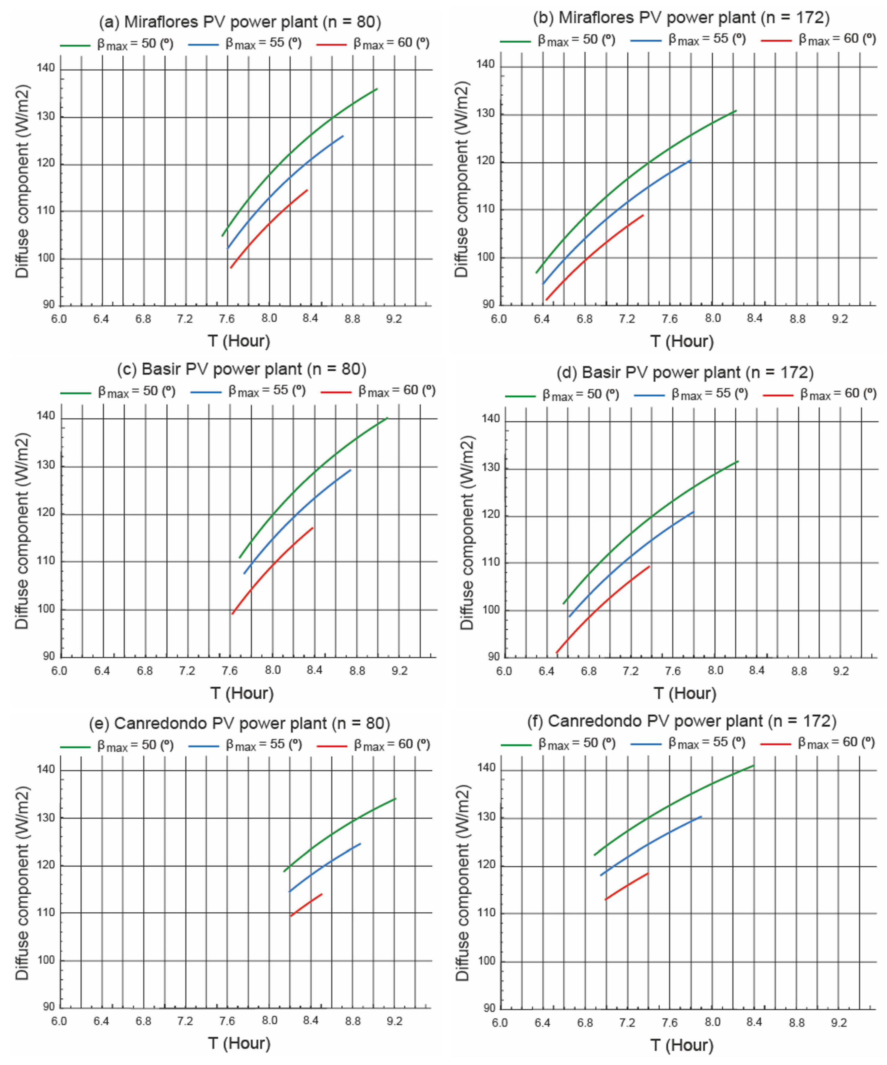
If the diffuse component is predominant, the longer the duration of operation in static mode, the worse the performance of the current scenario. Since the current scenario starts the normal tracking mode first, the rest of the scenarios follow in the horizontal position that favours the diffuse component.

(ii)

During the static operation mode, on day $n=80$, the Miraflores $PV$ power plant has the smallest diffuse component. This favours the current scenario. In contrast, the Canredondo $PV$ power plant has the highest diffuse component. This fact favours a scenario that is different from the current one.

(iii)

During the static operation mode, on day $n=172$, the Miraflores $PV$ power plant has the smallest diffuse component. This fact favours the current scenario. In contrast, the Canredondo $PV$ power plant has the highest diffuse component. This fact favours a scenario that is different from the current one.

It can be concluded that the high values of the beam component favour the current scenario. In contrast, high values of the diffuse component favour scenarios that are different from the current scenario.

4. Conclusions

This paper presents an energy study on the influence of the movement limit of a horizontal single-axis tracker. The study focused on three photovoltaic power plants in Spain (Miraflores $PV$ power plant, Basir $PV$ power plant, and Canredondo $PV$ power plant). Four evaluation indicators (annual energy loss, daily energy loss, beam component, and diffuse component) and ten movement limits, ranging from $\pm 50$ ($°$) to $\pm 60$ ($°$), were analysed. In Spain, $PV$ power plants usually have a movement limit of $\pm 60$ ($°$). Several specific codes were developed to determine the components of the incident solar irradiance (beam component, diffuse component, and reflected component) and the periods of operation (normal tracking mode, backtracking mode, and static mode). The codes were performed with $Mathematica$ software. The current scenario ($\pm 60$ ($°$)) was used as a basis for the comparison. The main conclusions of this study are summarised as follows:

(i)

In all three $PV$ power plants analysed, the energy loss per square metre is small, but as the surface of the $PV$ field is large, these losses cannot be neglected. The choice of a movement limit different from the optimum produces energy losses that cannot be neglected, taking into account the large surface area of the $PV$ field. The surface area of the $PV$ field at the Miraflores $PV$ power plant is 105,109.81 (m²), and at the Basir and Canredondo $PV$ power plant it is (m²) 95,616.64 and 105,012.67 (m²), respectively.

(ii)

Although most $PV$ power plants in Spain use a movement limit of $\pm 60$ ($°$), a study on the optimum movement limit is necessary. The movement limit of the Canredondo $PV$ power plant is currently $\pm 60$ ($°$). It has been demonstrated that the movement limit is not optimised. The annual energy loss is $18.49$ (MWh). Therefore, it is necessary to calculate the optimal movement limit for each location under study, as the annual losses of the incident energy are not negligible. In contrast, the Miraflores and Basir $PV$ power plants do use an optimal movement limit.

(iii)

In all locations, the current scenario has the shortest static mode operation period. Therefore, when the current scenario starts the normal tracking mode (where the beam component is maximised), the other two scenarios remain in the operation static mode, impairing the incidence of the beam component on the $PV$ field.

(iv)

Considering the current scenario as a basis for comparison, the most favourable results for this scenario are obtained in the summer months (low $k_d$) and the least favourable in the spring months (high $k_d$).

(v)

If the beam component is predominant, the longer the duration of operation in static mode, the better the performance of the current scenario. Since the current scenario first starts the normal tracking mode that favours the beam component, the rest of the scenarios follow in the horizontal position.

(vi)

If the diffuse component is predominant, the longer the duration of operation in static mode, the worse the performance of the current scenario. Since the current scenario starts the normal tracking mode first, the rest of the scenarios follow in the horizontal position that favours the diffuse component.

(vii)

It can be concluded that high values of the beam component favour the current scenario. In contrast, high values of the diffuse component favour scenarios other than the current scenario.

This study achieved its objectives and can be replicated anywhere in the world, with the only limitation being the knowledge of the meteorological data of the location. As the basis of the study is the calculation of the incident solar irradiance on the $PV$ field, the lack of solar irradiance data would be the only limitation of this study. It is also true that such data are available in most locations.

References

- IEA. Electricity 2024. Available online: https://iea.blob.core.windows.net/assets/18f3ed24-4b26-4c83-a3d2-8a1be51c8cc8/Electricity2024-Analysisandforecastto2026.pdf (accessed on 23 November 2024).
- IEA. World Energy Outlook 2023. Available online: https://www.iea.org/reports/world-energy-outlook-2023?language=es (accessed on 23 November 2024).
- European Union. Directive 2018/2001/EC, on the Promotion of the Use of Energy from Renewable Sources. 2018. Available online: https://eur-lex.europa.eu/eli/dir/2018/2001/oj/eng (accessed on 23 November 2024).
- Future Market Insights, Solar Trackers Market: Solar Trackers Market Analysis by Single-Axis and Dual-Axis for 2023 to 2033. Available online: https://www.futuremarketinsights.com/reports/solar-trackers-market#:\protect\char126\relax:text=The%20global%20solar%20trackers%20market,to%20renewable%20energy%20sources%20grows (accessed on 23 November 2024).
- Gonvarri Solar Steel. Available online: https://www.gsolarsteel.com/ (accessed on 23 November 2024).
- Barbón, A.; Fortuny Ayuso, P.; Bayón, L.; Silva, C.A. A comparative study between racking systems for photovoltaic power systems. Renew. Energy 2021, 180, 424–437. [Google Scholar] [CrossRef]
- Martín-Martínez, S.; Cañas-Carretón, M.; Honrubia-Escribano, A.; Gómez-Lázaro, E. Performance evaluation of large solar photovoltaic power plants in Spain. Energy Convers. Manag. 2019, 183, 515–528. [Google Scholar] [CrossRef]
- Antaisolar. Available online: https://www.antaisolar.com/ (accessed on 23 November 2024).
- Barbón, A.; Carreira-Fontao, V.; Bayón, L.; Silva, C.A. Optimal design and cost analysis of single-axis tracking photovoltaic power plants. Renew. Energy 2023, 211, 626–646. [Google Scholar] [CrossRef]
- Duffie, J.A.; Beckman, W.A. Solar Engineering of Thermal Processes, 4th ed.; John Wiley & Sons: New York, NY, USA, 2013. [Google Scholar]
- Ledesma, J.R.; Lorenzo, E.; Narvarte, L. Single-axis tracking and bifacial gain on sloping terrain. Prog. Photovoltaics Research Appl. 2024, 33, 309–325. [Google Scholar] [CrossRef]
- López, M. Detection of tracker misalignments and estimation of cross-axis slope in photovoltaic plants. Solar Energy 2024, 272, 112490. [Google Scholar] [CrossRef]
- Keiner, D.; Walter, L.; ElSayed, M.; Breyer, C. Impact of backtracking strategies on techno-economics of horizontal single-axis tracking solar photovoltaic power plants. Sol. Energy 2024, 267, 112228. [Google Scholar] [CrossRef]
- Casares de la Torre, F.J.; Varo, M.; López-Luque, R.; Ramírez-Faz, J.; Fernández-Ahumada, L.M. Design and analysis of a tracking / backtracking strategy for PV plants with horizontal trackers after their conversion to agrivoltaic plants. Renew. Energy 2022, 187, 537–550. [Google Scholar] [CrossRef]
- Barbón, A.; Bayón-Cueli, C.; Bayón, L.; Carreira-Fontao, V. Study of the influence of the motion limit of a horizontal single-axis tracker on the annual incident energy in a PV power plant. In Proceedings of the 2024 IEEE International Conference on Environmental and Electrical Engineering (EEEIC2024), Rome, Italy, 17–20 June 2024; pp. 1–4. [Google Scholar]
- Anderson, K.S.; Jensen, A.R. Shaded fraction and backtracking in single-axis trackers on rolling terrain. J. Renew. Sustain. Energy 2024, 16, 023504. [Google Scholar] [CrossRef]
- Huang, B.; Huang, J.; Xing, K.; Liao, L.; Xie, P.; Xiao, M.; Zhao, W. Development of a solar-tracking system for horizontal single-axis PV arrays using spatial projection analysis. Energies 2023, 16, 4008. [Google Scholar] [CrossRef]
- Alves Veríssimo, P.H.; Antunes Campos, R.; Vivian Guarnieri, M.; Alves Veríssimo, J.P.; do Nascimento, L.R.; Rüther, R. Area and LCOE considerations in utility-scale, single-axis tracking PV power plant topology optimization. Sol. Energy 2020, 211, 433–445. [Google Scholar] [CrossRef]
- Sun, L.; Bai, J.; Kumar Pachauri, R.; Wang, S. A horizontal single-axis tracking bracket with an adjustable tilt angle and its adaptive real-time tracking system for bifacial PV modules. Renew. Energy 2024, 221, 119762. [Google Scholar] [CrossRef]
- Kamran Khan, M.; Hamza Zafar, M.; Riaz, T.; Mansoor, M.; Akhtar, N. Enhancing efficient solar energy harvesting: A process-in-loop investigation of MPPT control with a novel stochastic algorithm. Energy Convers. Manag. 2024, 21, 100509. [Google Scholar] [CrossRef]
- Tina, G.M.; Bontempo Scavo, F.; Micheli, L.; Rosa-Clot, M. Economic comparison of floating photovoltaic systems with tracking systems and active cooling in a Mediterranean water basin. Energy Sustain. 2023, 76, 101283. [Google Scholar] [CrossRef]
- Antonanzas, J.; Urraca, R.; Martinez-de-Pison, F.J.; Antonanzas, F. Optimal solar tracking strategy to increase irradiance in the plane of array under cloudy conditions: A study across Europe. Sol. Energy 2018, 163, 122–130. [Google Scholar] [CrossRef]
- López, M.; Soto, F.; Hernández, Z.A. Assessment of the potential of floating solar photovoltaic panels in bodies of water in mainland Spain. J. Clean. Prod. 2022, 340, 130752. [Google Scholar] [CrossRef]
- Makhdoomi, S.; Askarzadeh, A. Impact of solar tracker and energy storage system on sizing of hybrid energy systems: A comparison between diesel/PV/PHS and diesel/PV/FC. Energy 2021, 231, 120920. [Google Scholar] [CrossRef]
- Zhu, Y.; Liu, J.; Yang, X. Design and performance analysis of a solar tracking system with a novel single-axis tracking structure to maximize energy collection. Appl. Energy 2020, 264, 114647. [Google Scholar] [CrossRef]
- Farahat, A.; Kambezidis, H.D.; Almazroui, M.; Ramadan, E. Solar Energy Potential on Surfaces with Various Inclination Modes in Saudi Arabia: Performance of an Isotropic and an Anisotropic Model. Appl. Sci. 2022, 12, 5356. [Google Scholar] [CrossRef]
- Peña-Cruz, M.I.; Díaz-Ponce, A.; Sánchez-Segura, C.D.; Valentín-Coronado, L.; Moctezuma, D. Short-term forecast of solar irradiance components using an alternative mathematical approach for the identification of cloud features. Renew. Energy 2024, 237, 121691. [Google Scholar] [CrossRef]
- Salazar, G.; Gueymard, C.; Bezerra Galdino, J.; Castro Vilela, O. Solar irradiance time series derived from high-quality measurements, satellite-based models, and reanalyses at a near-equatorial site in Brazil. Renew. Sustain. Energy Rev. 2020, 117, 109478. [Google Scholar] [CrossRef]
- Barbón, A.; Fortuny Ayuso, P.; Bayón, L.; Fernández-Rubiera, J.A. Predicting beam and diffuse horizontal irradiance using Fourier expansions. Renew. Energy 2020, 154, 46–57. [Google Scholar] [CrossRef]
- Jallal, M.A.; El Yassini, A.; Chabaa, S.; Zeroual, A.; Ibnyaich, S. Ensemble learning algorithm-based artificial neural network for predicting solar radiation data. In Proceedings of the IEEE International Conference on Decision Aid Sciences and Application (DASA), Sakheer, Bahrain, 8–9 November 2020; pp. 526–531. [Google Scholar]
- PVGIS. Joint Research Centre (JRC). 2024. Available online: https://re.jrc.ec.europa.eu/pvg_tools/ (accessed on 23 November 2024).
- PVSyst. Available online: https://www.pvsyst.com/ (accessed on 10 January 2025).
- Kambezidis, H.D. The solar radiation climate of Athens: Variations and tendencies in the period 1992–2017, the brightening era. Sol. Energy 2018, 173, 328–347. [Google Scholar] [CrossRef]
- Kong, H.J.; Kim, J.T. A Classification of real sky conditions for Yongin, Korea. In Sustainability in Energy and Buildings. Smart Innovation, Systems and Technologies; Springer: Berlin/Heidelberg, Germany, 2013; Volume 22, pp. 1025–1032. [Google Scholar]