FTGM: Fast Transformer-Based Global Matching for Particle Image Velocimetry

Abstract

The integration of deep learning with optical flow estimation in Particle Image Velocimetry (PIV) represents an emerging solution. Extensive research indicates that deep learning has potential to match or outperform state-of-the-art classical algorithms in efficiency, accuracy, and spatial resolution. However, current learning-based methods, which rely on cost volumes and convolutions for flow regression, are limited to local correlations. This limitation hinders the capture of global information. While extensive iterative refinements enhance the quality of prediction flows, they also result in a linear increase in inference time. To enhance both efficiency and accuracy, we propose a global matching method for PIV. This method directly compares feature similarities to identify correspondences between images and generate estimated flows. The underlying idea is to first extract initial features of particle image pairs, then enhance these features through a Transformer specifically designed for PIV, and perform operations for feature correlation matching, followed by global optical flow propagation and optimization. Additionally, higher-resolution features are introduced for refinement. By employing both synthetic and experimental data, including benchmark sets and data from turbulent wave channel flow experiments, we demonstrate that global matching method in PIV achieves superior efficiency and accuracy compared to existing learning-based methods.

1. Introduction

Particle Image Velocimetry (PIV), a pivotal tool in contemporary fluid dynamics research, offers a non-invasive and high-precision method for the quantitative measurement of the full-field velocity field [1,2]. It achieves this by capturing and analyzing images of a fluid containing small particles at a short time interval, typically on the order of microseconds, to extract detailed information about the velocity field.

The traditional methods of PIV estimation predominantly consist of cross-correlation and optical flow methodologies. The cross-correlation method (CC) [3], which enjoys widespread adoption, typically involves segmenting PIV images into smaller sub-regions, referred to as interrogation areas (IAs). By computing the correlation within the image pairs for these interrogation areas, the direction of maximum match is ascertained, which then determines the displacement at the centroid of each interrogation area. The window deformation iterative multi-grid (WIDIM) method [4], a representative technique in the realm of Particle Image Velocimetry, employs an iterative multi-grid refinement strategy that dynamically narrows the size of the interrogation window during the iterative query process, thereby markedly enhancing the spatial resolution and precision of numerical interrogation schemes, as evidenced by its commendable performance in international PIV challenge assessments. However, the cross-correlation method is based on the assumption of uniform motion. This means that all particles within an interrogation area are assumed to exhibit a consistent motion state. The method faces challenges when dealing with complex flow scenarios. It tends to partially lose the anisotropy of the flow field and the abrupt changes in velocity. This limitation, which restricts the output to a single vector per window, further restricts the spatial resolution of the output velocity field to the scale of the interrogation area, consequently hindering the algorithm’s ability to accurately capture fine-scale vortex structures that are smaller than the interrogation area itself.

Another significant approach, the optical flow method [5,6], is capable of yielding dense velocity vector fields with single-pixel resolution. This improves the measurement of small-scale fine structures and compensating for the deficiencies of correlation-based methods. Initially proposed by Horn and Schunck in their seminal work [5], which has since become a cornerstone in the field. This method has also garnered considerable interest among fluid dynamics experimentalists. Addressing the inadequacy of classic optical flow models to adapt to fluid dynamics, researchers often consider incorporating fluid dynamics prior knowledge into the model to optimize the data term (based on brightness constancy assumption) and regularization terms in the objective function using physical equations of fluid mechanics [7,8]. However, the variational optimization required by optical flow algorithms is computationally intensive and time-consuming. There remains room for improvement in optical flow algorithms.

The emergence of deep learning (DL) has catalyzed the development of innovative approaches to address the existing challenges. Deep optical flow models, which have made significant strides in computer vision, have demonstrated remarkable performance [9,10,11,12,13,14,15,16,17,18,19]. These advancements have inspired researchers to adapt and modify high-performing models for Particle Image Velocimetry estimation. Early efforts primarily focused on model stacking to enhance precision [20,21,22,23,24]; however, these models were complex and suffered from significant parameter redundancy. The introduction of the Recurrent All-Pairs Field Transforms (RAFT) framework [19], with its outstanding performance, established a foundational architecture for learning-based optical flow estimation methods. This development has spurred the emergence of numerous improved PIV estimation methods based on this architecture [25,26,27], collectively termed RAFT-PIV. RAFT continues to be recognized as the most advanced deep optical flow architecture for PIV [28]. The application of deep optical flow models in PIV has subsequently expanded into a broader range of domains [29,30,31,32,33,34,35,36]. Nonetheless, these methods involve extensive iterative refinement processes, which result in a linear increase in inference time with the number of iterations. There remains considerable potential for enhancing computational efficiency and precision.

In this paper, we propose a Fast Transformer-based Global Matching (FTGM) method for PIV estimation, which redefines the optical flow estimation as a global matching problem (Figure 1). FTGM provides a fresh perspective on PIV estimation.

In summary, our major contributions can be summarized as follows:

• We apply the global matching approach to PIV estimation, thereby refining the learning-based flow regression methods. This approach allows for a simpler PIV estimation pipeline while achieving higher precision in displacement estimation and greater computational efficiency.
• Given the intrinsic differences between PIV datasets and optical flow datasets, we have tailored a Transformer incorporating self-attention, cross-attention, and a feed-forward network specifically for enhancing the features of PIV images, thereby obtaining high-quality discriminative features essential for accurate matching.
• We further introduce a refinement step that utilizes higher-resolution features to improve estimation accuracy. This process can reuse the FTGM framework for residual flow estimation, thereby reducing network complexity and parameters.

2. Related Work

In recent years, deep learning-based optical flow techniques have exhibited the potential to match and outperform the efficiency, accuracy, and spatial resolution of classical state-of-the-art algorithms. In a pioneering study [20], the potential of using artificial neural networks (ANNs) for Particle Image Velocimetry was first explored, with attempts to apply Convolutional Neural Networks (CNNs) and Fully Convolutional Neural Networks (FCNNs) to PIV and validate their effectiveness through synthetic images and real-world data. Although ANNs’ performance in some aspects still lags slightly behind traditional methods, they show promise in handling complex flows and enhancing spatial resolution.

Lee et al. [21] designed a cascaded PIV deep convolutional neural network (PIV-DCNN) that demonstrated improved spatial resolution. This method involves a four-stage regression structure, where each level of the network is trained to predict displacement from input particle image block pairs, without any pre-established model assumptions. However, the model cannot output a dense velocity field, and the computational process is highly time-consuming. Cai et al. [22] enhanced the FlowNetS [9] model for PIV estimation by incorporating deconvolutional layers into the final stage of the model to achieve high-resolution velocity fields at the pixel level. Employing a similar strategy, they also improved the LiteFlowNet [11], resulting in PIV-LiteFlowNet [24], which further increased estimation accuracy. However, these methods further increased the size of the models, introducing a significant amount of parameter redundancy.

A significant advancement in the task of optical flow estimation in computer vision is the RAFT [19], achieving state-of-the-art performance on benchmark datasets. This framework employs weight sharing and recurrent mechanisms to avoid the complexity and hyperparameter sensitivity of traditional multi-stage cascaded networks. Consequently, numerous improvements and applications based on this model have emerged in PIV research, with the 4D correlation volumes and iterative update units becoming widely used structures in PIV estimation. Yu et al. proposed LightPIVNet [25], which reduces the number of parameters by 47% and computation time by 14% compared to PIV-LiteFlowNet-en. The improvement strategy involves reducing the number of residual units in the feature encoder of RAFT from three to two and changing the output resolution of the feature maps from the original 1/8 to 1/4. This change provides a higher resolution for subsequent iterative optimization processes, retaining more details and enhancing the precision of PIV estimation while reducing the number of parameters. Subsequently, Lagemann et al. [26] adapted RAFT to RAFT-PIV, achieving state-of-the-art accuracy and performance in PIV using optical flow estimation. Lagemann et al. [27] undertook a study to evaluate the generalizability and robustness of RAFT-PIV, conducting extensive tests across a diverse array of real-world PIV datasets and examining the impact of varying PIV parameters in synthetically derived datasets. Yuvarajendra et al. [28] conducted an investigation into the impact of modified input particle image properties, such as particle diameter, Reynolds number, and particle concentration (particles per interrogation area), on the detection performance of RAFT-PIV using cylindrical flow around an obstacle. Lagemann et al. [29] constructed the WSSflow framework based on RAFT components, which offers significant advantages in providing high spatiotemporal resolution of wall shear stress (WSS) dynamics, particularly in near-wall regions.

Beyond these, other notable deep learning-based algorithms for flow estimation in PIV exist. Zhang et al. [30] introduced UnLiteFlowNet-PIV, while Lagemann et al. [31] proposed an unsupervised deep learning algorithm named URAFT-PIV and introduced a proxy loss function. Yu et al. [32] developed Deep-TRPIV, a novel multi-frame architecture designed for the prediction of optical flow in sequences of particle images, inspired by the RAFT framework. Han et al. [33] introduced ARaft-FlowNet, a deep recurrent network based on the RAFT architecture with an attention mechanism, improving trace particle motion recognition. Lagemann et al. introduced latent dynamical models [34] to extract underlying physical mechanisms. They plan to further enhance their work by integrating the URAFT-PIV network with causal risk frameworks [35]. This integration will enable the direct learning of causal flow relations from particle images. According to their speculation, (U)RAFT-PIV is also capable of deriving important flow quantities [36], such as the instantaneous wall-shear stress distribution over a relatively large spatial extent.

Despite achieving significant performance improvements in various tasks by using learning-based flow regression methods, these studies still rely on cost volumes and iterative refinements as primary guiding principles. These principles involve applying convolutions to different local cost volumes at various iterative stages to progressively expand the global search space. However, the extensive sequential refinements lead to a linear increase in processing time, limiting their potential for application in practical systems. Consequently, the question arises whether it is possible to achieve high precision and efficiency without relying on a large number of iterations.

3. Approach

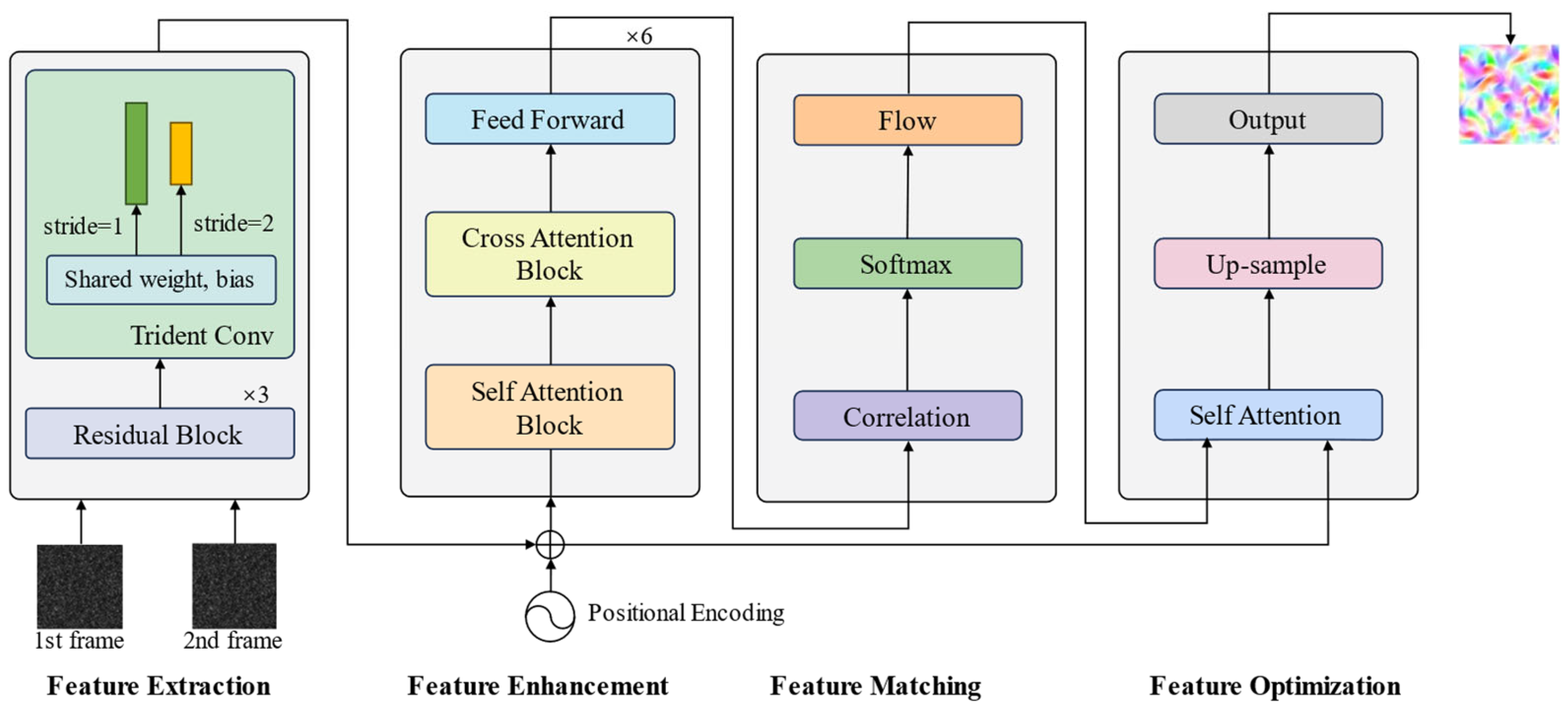
We propose a fast Transformer-based global matching framework (FTGM) that replaces the previously widely used iterative refinement strategies in PIV estimation with a simple and effective Transformer and global matching structure. FTGM comprises feature extraction, feature enhancement, global matching, and flow propagation. Figure 1 provides an overview of FTGM, and each module is detailed in the following sections.

3.1. Feature Extraction and Enhancement

Given two frames $I_1$ and $I_2$, FTGM first employs a feature extraction backbone composed of a three-layer residual network with weight-sharing to obtain downsampled initial features $F_1$, $F_2$. The essence of global matching fundamentally lies in identifying corresponding pixels between frames, with the key challenge being the enhancement of feature distinctiveness to facilitate the matching. To account for their interdependencies more comprehensively, the Transformer is a natural choice. It excels at capturing the reciprocal relationships between two sets through its attention mechanism.

Position Embedding. Since the features $F_1$ and $F_2$ have no notion of the spatial position, it is imperative to inject positional information for each pixel. In this work, we employ fixed 2D sine and cosine functions as positional encodings of different frequencies (following DETR [37]):

$$\left\{\begin{array}{l}P{E}_{(pos,2i)}=\sin (pos/10,{000}^{2i/d_{\mathrm{mod}el}})\\ P{E}_{(pos,2i+1)}=\cos (pos/10,{000}^{2i+1/d_{\mathrm{mod}el}})\end{array}\right.,$$

(1)

where $pos$ is the position of the pixel, $i$ represents the dimensional information, and for any offset $k$, the positional encoding $P{E}_{pos+k}$ can be expressed as a linear function of $P{E}_{pos}$. The incorporation of positional information not only considers the similarity of features but also their spatial distances, which aids in resolving ambiguities and enhancing the performance.

Customized Transformer. Considering the fundamental differences between PIV data and the optical flow datasets from natural scenes, we define a Transformer block to improve the quality of the initial features (Figure 2). Features $F_1$ and $F_2$ are concatenated and symmetrically processed to serve as the source and target, respectively. The source is fed into the self-attention layer. Unlike the standard Transformer, we omit the feed-forward network in the self-attention layer to ensure the “purity” of the model’s feature representation based on the input sequence’s inherent structure and internal dependencies, a concept akin to the functionality of a context encoder. In the cross-attention layer, the output of the self-attention layer interacts with the original target features. In the FFN layer, the concatenated result of the cross-attention layer’s output and the source undergoes dimension expansion and non-linear activation, allowing the FFN to fuse information from both the input sequence and the encoder output, thereby generating richer feature representations. Residual connections and layer normalization maintain numerical stability and effective information propagation.

Attention Mechanism. The attention mechanism, central to the Transformer architecture, is capable of capturing dependencies between any two positions within the input image. Given query vectors $Q\in {ℝ}^{d_q\times d_m}$, key vectors $K\in {ℝ}^{d_k\times d_m}$, and value vectors $V\in {ℝ}^{d_v\times d_m}$, where $d_m$ is the feature dimension, the attention module computes the similarity between the Q and K and then applies a softmax function to obtain the weights on the value, and the attention is calculated as

$$Attention(Q,K,V)=softmax(Q{K}^T/\sqrt{d_m})\cdot V.$$

(2)

The attention weights determine the proportion of each value vector in the final output so that the model can focus on salient features for the current task and disregard irrelevant portions. For more details about attention, please refer to [15].

Shifted Local Window Attention. In the context of Transformer architectures, the computational expense of the attention mechanism is considerable, stemming from its quadratic computational complexity when dealing with input features. To enhance computational efficiency, we implement a strategy that employs a fixed count of local-window attentions. We segment the feature map, which is $H$ by $W$ in dimensions, into smaller $K$ by $K$ grids and perform self- and cross-attention computations within each localized grid independently. For every two consecutive local windows, we introduce cross-attention by using a window with a shift offset $\left(\frac{H}{2K},\frac{W}{2K}\right)$ in the even-numbered Transformer blocks, thereby facilitating information fusion across windows.

3.2. Global Matching and Flow Propagation

Considering two feature sets ${\stackrel{\wedge }{F}}_1$ and ${\stackrel{\wedge }{F}}_2$ that have been enhanced by the Transformer block, their corresponding pixels should exhibit a high degree of similarity. To achieve this, we construct a similarity matrix $C$ for the feature maps, a process that entails computing the feature similarity between each pixel in $F_1$ with respect to all pixels in $F_2$.

$$C(i,j,u,v)={\stackrel{\wedge }{F}}_1(i,j)\cdot {\stackrel{\wedge }{F}}_2(u,v)/\sqrt{d_m},$$

(3)

where $(i,j)$ and $(u,v)$ refer to locations in ${\stackrel{\wedge }{F}}_1$ and ${\stackrel{\wedge }{F}}_2$, and $1/\sqrt{d_m}$ is a normalization factor to counteract the effect of excessively large values resulting from the dot-product operation.

To identify the correspondence between pixels in the features, we employ a softmax operator [38] on the last two dimensions of $C$ to obtain a matching distribution,

$$M=softmax(C),$$

(4)

and then use this distribution as weights to perform a weighted average with the initialized 2D pixel grid coordinates $G$ to derive a predicted grid coordinate,

$$\stackrel{\wedge }{G}=M\cdot G,$$

(5)

and by computing the difference between the grid coordinates, the optical flow can be derived:

$$V=\stackrel{\wedge }{G}-G,$$

(6)

Finally, we employ a self-attention layer to propagate high-quality flow predictions from matched pixels to unmatched ones by measuring the self-similarity of features:

$$\stackrel{\wedge }{V}=Attention({\stackrel{\wedge }{F}}_1,{\stackrel{\wedge }{F}}_1,)\cdot V-G.$$

(7)

3.3. Upsampling

The network outputs optical flow at a 1/8 resolution. To match the resolution of the ground truth, we employ convex upsampling, a method proposed in [12], to upsample the flow prediction fields, the core principle of which involves treating the full-resolution optical flow as a convex combination of 3 × 3 weighted grids predicted by the matching distribution. Specifically, when upsampling optical flow predicted at 1/8 resolution, each pixel needs to be expanded into 64 (8 × 8) pixels. The convex upsampling module predicts the weights for each new pixel in the upsampled optical flow predictions through two convolutional layers, followed by a softmax activation at the end. These weights are then used to combine the low-resolution optical flow field in a weighted manner to produce a high-resolution optical flow field.

3.4. Refinement

The model framework generates flow predictions based on features at 1/8 resolution. To further improve performance, aligning with the principles of ideal pyramid network structures, we employ a weight-sharing backbone network to produce features at 1/4 and 1/8 resolutions, with strides of 1 and 2, respectively, in the last convolutional layer. The specific refinement process is as follows: the framework initially generates a flow prediction at 1/8 features, which is then upsampled to 1/4 resolution. This flow field is utilized to perform a warp operation on the feature map of the second frame. Subsequently, Transformer-based feature enhancement and global matching are conducted to learn a residual flow. Finally, the flow sum is subjected to convex upsampling, yielding a full-resolution optical flow field.

3.5. Training Loss

We follow RAFT and supervise our network on the ${\mathcal{l}}_1$ distance between all flow predictions and ground truth flow, with exponentially increasing weights. The training loss is defined as

$$L={\displaystyle \sum _{i=1}^N{\gamma }^{N-i}{‖V_{gt,i}-V_{es,i}‖}_1},$$

(8)

where $N$ is the number of flow predictions including the intermediate and final ones, and we set $\gamma$ to 0.9 in our experiments.

4. Experiments

4.1. Overview of Datasets

PIV Dataset I—involves extensive public PIV data. These datasets originate from a publicly accessible database that serves as a benchmark for PIV algorithms [22]. The dataset includes five both well-known and realistic flow scenarios, such as backward stepping flow (backstep), vortex shedding over a circular cylinder (cylinder), 2D turbulent flow motion from direct numerical simulation (termed DNS turbulence), surface quasi-geostrophic (SQG) model of sea flow, and different flows from the Johns Hopkins Turbulence Database (JHTDB). The particle images are artificially synthesized with a displacement range of approximately ±10 pixels. The dataset is distinguished by a high seeding density and a high signal-to-noise ratio (SNR), indicating nearly ideal experimental conditions.

PIV Dataset II—encompassing a vast array of flow conditions to bolster model training and parameter optimization—enhances model generalization through its rich and extensive compilation of scenarios. The dataset cited in [25] features a displacement range of ±10 pixels, with new particle images synthesized to include vortices, point sources, point sinks, dipole flow fields, and square cavity flows. To emulate real-world fluid dynamics, these images incorporate Gaussian noise of diverse magnitudes and random spatial distributions of light intensity.

PIV Dataset III—featuring datasets with real-world constraints—reflects the practical challenges of PIV equipment [26], where both internal and external noise sources make it nearly impossible to obtain high-quality images as seen in PIV Datasets I and II. This dataset simulates image acquisition from actual devices, similar to Dataset I, but with a particle displacement range of ±24 pixels, reduced particle density, lowered signal-to-noise ratio, and added camera noise.

PIV Dataset IV—advancing to real-world test scenarios—further evaluates generalization capabilities through predictions on synthetic data and experimental test cases beyond the confines of the training set, which include the following:

• Realistic vortex pair flow images [39], used to study the interaction between flow vortex structures. The double-helical vortices are generated by the nozzle, which has a relatively stable flow field with fine structures near the nozzle position, making it highly suitable for PIV analysis with particle images of good imaging quality.
• Actual Karman vortex street images [40], which form a series of alternating vortices downstream of an obstacle (such as a cylinder) when a fluid flows past it. This flow field is a classic phenomenon in fluid dynamics, often used to study fluid separation, vortex shedding, and turbulence characteristics. The image, sourced from PIVLab [41], is used to demonstrate how the PIV method can be employed to analyze and visualize the flow field of the Karman vortex street.
• Spatial resolution images. The test case originates from Group A-4 of the public data of the Third International PIV Fluid Measurement Conference [42], specifically for evaluating the spatial resolution and the fine measurement performance of vortex structures using test algorithms.
• Turbulent wave channel flow—characterized by the presence of favorable and adverse pressure gradients [26], which are crucial for understanding the evolution of turbulent scales under the influence of local pressure gradients. By evaluating PIV optical flow models within this flow field, we can assess the performance of the methods in handling complex flow patterns, such as flow separation, reattachment, and periodic vortex shedding.

4.2. Implementation Details

Training Details: Our method is implemented in the open-source framework PyTorch (v2.5.1), employing a convolutional backbone network analogous to that of RAFT, which outputs feature dimensions of 128. We stack six Transformer blocks. Among these, the final upsampling layer utilizes a convex upsampling technique, while the preceding upsampling layers employ bilinear interpolation for original image enhancement. We train our model on an NVIDIA A100 GPU 80GB with a batch size of 12. For training, the model is initialized from scratch with random weights. Following previous methods, we first train our model on the baseline and validate its performance on a test set with the same distribution. We employ the AdamW optimizer with a weight decay of 0.00005 and use the PyTorch OneCycle learning rate scheduler, setting the maximum learning rate to 4 × 10⁻⁴ and training for 500,000 steps.

Assessment Metrics. For quantitative evaluation, we adopt the commonly used metric in PIV estimation, i.e., average endpoint error (AEE), which is defined as the average ${\mathcal{l}}_2$ distance between the final predicted and ground-truth optical flow over all pixels,

$$AEE={‖V_{es,N}-V_{gt}‖}_2$$

(9)

4.3. Quantitative Evaluations

RAFT256-PIV [26] currently represents the state of the art in performance within benchmark evaluations. In the tests, this method serves as the baseline. We adhere to the benchmark evaluation procedures detailed in [26] for all subsequent assessment tests.

Initially, our model FTGM is trained on the public benchmark dataset PIV Dataset I.

Table 1. Average endpoint error for all test cases of PIV Dataset I.

Methods	Backstep	Cylinder	DNS Turbulence	JHTDB	SQG
WIDIM [4]	3.4	8.3	30.4	8.4	45.7
Horn–Schunck optical flow [5]	4.5	7.0	52.5	6.9	15.6
PIV-NetS-noRef [22]	13.9	19.4	52.5	24.7	52.5
PIV-NetS [22]	7.2	11.5	28.2	15.5	29.4
PIV-LiteFlowNet [24]	5.6	8.3	19.6	10.4	20.0
PIV-LiteFlowNet-en [24]	3.3	4.9	12.2	7.5	12.6
UnLiteFlowNet-PIV [30]	10.1	7.8	13.5	9.6	19.7
RAFT256-PIV [26]	0.9	1.6	10.0	15.7	8.4
FTGM-PIV	1.0	2.3	4.3	6.2	11.8
FTGM-PIV-Ref	0.8 *	2.6	3.0	4.2	7.2 *

* All methods listed are trained and tested based on PIV Dataset I. The error unit is set to pixels per 100 pixels for easier comparison. The best and runner-up results are highlighted in bold and underlined, respectively. For these metrics, lower is better.

presents the test results for FTGM alongside a series of existing methods, specifically the average AEE for each test case in the test set. Without any refinements, our method’s performance matches or exceeds that of the RAFT256-PIV method with iterative optimization (iteration = 16). After incorporating a single refinement, namely the addition of 1/4 resolution features, our method achieves state-of-the-art performance on the benchmark set. Our method achieved an average endpoint error of 0.8 px on backstep, 3.0 px on DNS turbulence, 4.2 px on JHTDB, and 7.2 px on SQG, with the error unit is set to pixels per 100 pixels. These results represent reductions of 11%, 70%, 73%, and 14% in AEE compared to RAFT256-PIV, respectively. The FTGM model thus exhibits superior estimation accuracy. This significant improvement validates our approach of formulating PIV estimation as a global matching problem and demonstrates that substantial enhancements can be achieved after a single refinement.

To further validate the performance of FTGM across a spectrum of flow conditions, ranging from simple to complex flows, we trained and tested the FTGM model alongside the state-of-the-art model RAFT256-PIV on the PIV Dataset II, with the results presented in

Table 2. Average endpoint error for all test cases of PIV Dataset II.

Methods	Backstep	Cylinder	DNS Turbulence	JHTDB	SQG	Uniform	Cavity	Dipole	Sink	Source	Vortex
RAFT256-PIV [26]	3.52	2.92	11.9	14.5	3.97	14.8	6.40	2.11	1.09	1.21	3.03
FTGM-PIV	2.13	1.90	12.2	8.11	6.03	2.66	8.11	0.60	0.18	0.18	0.64
FTGM-PIV-Ref	1.73 *	1.57	10.4	6.50	3.85	1.67	5.88	0.44	0.25	0.26	0.94

* All methods listed are trained and tested based on PIV Dataset II. The error unit is set to pixels per 100 pixels for easier comparison. The best results are highlighted in bold. For these metrics, lower is better.

. Given that PIV Dataset II introduces random noise and random light intensity distribution in the particle images, it is anticipated that there would be an increase in error compared to the results in Table 1. It can be observed that all models perform best in simple flows, such as sink and source, and as the irregularity of the flow and the fine structures increase, the AEE tends to rise, as seen in DNS turbulence. Overall, the FTGM series of methods demonstrates excellent performance.

We trained our model and conducted tests on the challenging PIV Dataset III, which resembles real experimental data.

Table 3. Average endpoint error for all test cases of PIV Dataset III.

Methods	Backstep	Cylinder	DNS Turbulence	JHTDB	SQG	High-Displacement
RAFT256-PIV [26]	5.7	6.51	19.9	25.4	30.3	35.41
FTGM-PIV	1.55	3.54	13.7	11.6	20.63	34.39
FTGM-PIV-Ref	1.40 *	2.81	8.58	7.04	12.47	19.32

* All methods listed are trained and tested based on PIV Dataset II. The error unit is set to pixels per 100 pixels for easier comparison. The best results are highlighted in bold. For these metrics, lower is better.

summarizes the evaluation results. Consistent with expectations, the average endpoint error for all methods increased relative to the ideal PIV Dataset I. Nevertheless, our method still outperformed the RAFT256-PIV. To assess the capability of our method and baseline to estimate large displacements, we tested on a high-displacement dataset, which consists of particle image pairs with maximum displacements greater than ±16 pixels. The results demonstrated that the Transformer-based global matching method is superior to RAFT256-PIV, which maintains a sequential iteration strategy.

4.4. Qualitative Evaluations

We present the visualization of the estimated flow to clearly illustrate the improved performance of FTGM. For images larger than input size 256 × 256 pixels, we divide the images into patches of 256 × 256 pixels with a shift of 32 pixels. To cover all valid pixels, we use the reflect method for necessary edge padding during the patching process. After all patches have been predicted, they are unfolded back into the input image resolution.

Figure 3 presents several test cases from PIV Dataset I along with corresponding flow estimations of FTGM and RAFT256-PIV. In the cylinder case, it is observed that RAFT256-PIV has a stronger capability for capturing the edge details of flow-field structures compared to our method. However, in test samples such as SQG, JHTDB, and DNS turbulence, our method demonstrates smaller prediction errors, with this contrast being significant.

We also validate PIV algorithms using actual vortex pair images, with a size of 512 × 480 pixels. Figure 4 presents the estimated flows from different methods, where the background color indicates the magnitude of the flow field and the arrows represent the direction of velocity. It is evident that the listed algorithms are capable of accurately measuring both the magnitude and structure of the flow field. Figure 4 displays the result from PIVLab using an ensemble multipass FFT window deformation method [32] followed by bicubic interpolation to restore the original image resolution, which serves as the reference benchmark. The FTGM method exhibits anomalous value blocks locally, primarily due to low particle density in those areas, which prevents accurate estimation results. The RAFT256-PIV estimated flow demonstrates a certain global smoothing effect, which leads to irregularities in the nozzle edge structures. However, the estimated flow magnitude of RAFT256-PIV in the center of the vortex pair is lower than that estimated by traditional algorithms.

Figure 5 presents the Karman vortex street test image, sourced from PIVLab, with a size of 1024 × 765 pixels, and illustrates the comparative visualization of estimated flows from the RAFT256-PIV and FTGM methods. The reference results were obtained using the ensemble multipass FFT window deformation method in PIVLab and subsequently upsampled using bicubic interpolation. The flow estimated by the FTGM exhibits fully defined and clear structures. The absence of structure in the lower right corner of the flow field is primarily due to insufficient information at that location in the original image, which prevents accurate estimation. The flow estimated by RAFT256-PIV has numerous high estimates in the edge of the image and generates excessive details in the obstacle area, leading to an inability to discern the local structures of the flow field.

We evaluated our model on real-world experimental PIV turbulent wave channel flow and compared it with prediction results from a high-performance PIV post-processing method, PascalPIV, and the RAFT256-PIV method. The flow estimation results for PascalPIV were obtained from [26]. The image size is 2560 × 2160 pixels. When processing the full-resolution image using the same patch algorithm, the FTGM method took 43 s and 79 s (once refinement) on an NVIDIA A100, while the RAFT256-PIV took 113 s. Figure 6 illustrates the horizontal and vertical optical flow components estimated by different methods. FTGM showed consistent results with other methods in terms of flow-field structure estimation, whereas FTGM-PIV produced larger errors in magnitude. In contrast, FTGM-PIV-Ref achieved competitive performance after incorporating 1/4 resolution features for refinement, with its estimated results closely aligning with those of RAFT256-PIV and PascalPIV in both horizontal and vertical components. This demonstrates that the introduction of high-resolution features is effective for optimizing the estimation results of FTGM.

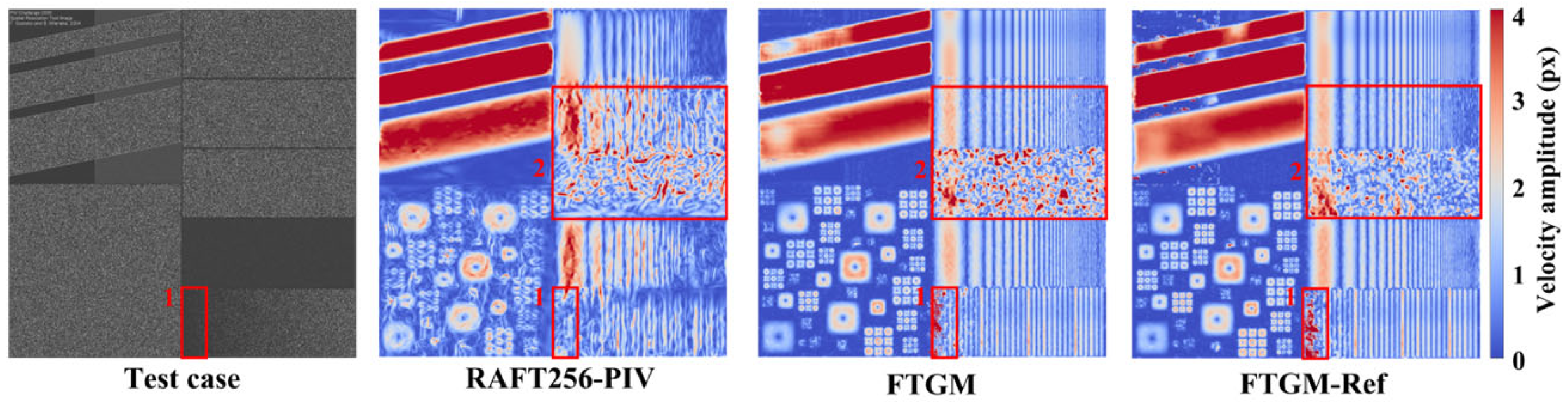
The ability of the PIV method to extract the motion of small-scale fluid structures from images, that is, their effective spatial resolution in predicting velocity fields, is one of the important metrics for evaluating PIV algorithms. We conducted tests on the PIV turbulence structure spatial resolution test image. We first present the global prediction results of the velocity magnitude for the full-resolution image (2000 × 2000 pixels) in Figure 7, processed using the same patch algorithm. It is evident that the FTGM method produces clear flow-field structures in the resolution image, whereas RAFT256-PIV captures more details within the flow field, missing the overall structure and also exhibiting more high estimates (as indicated by red rectangular 2 frames). 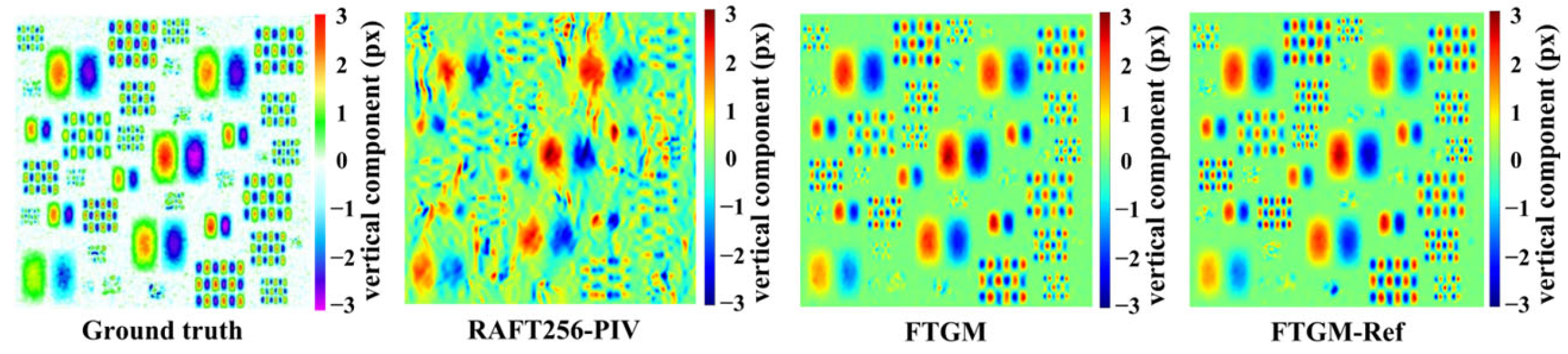Furthermore, we highlight the estimation results in the lower left corner of the image (1000 × 1000 pixels) shown in Figure 8, which shows the magnitude of the vertical velocity component. The results demonstrate that our method possesses clear structural representation capabilities.

4.5. Efficiency

The FTGM series of models has demonstrated not only improved performance but also reduced computational overhead. As shown in

Table 4. Comparisons of parameters and inference time.

Methods	Params (M)	Speed (ms)	GPU Memory (GB)	Match (ms)	Transformer (ms)	Iterations (ms)
RAFT256-PIV [26]	5.31	66	7.16	-	-	56
FTGM-PIV	4.68 (11.8% ↓)	14 (78.8% ↓)	7.11	0.35	9.5	-
FTGM-PIV-Ref *	4.72 (11.1% ↓)	30 (54.5% ↓)	20.62	4.5	20.5	-

* All models were trained on PIV Dataset I, utilizing an NVIDIA A100. Inference times were measured on an NVIDIA GTX 3080 platform. “Match” and “Transformer” denote the inference durations of the corresponding components within the FTGM, while “iterations” refers to the time taken for 16 update unit iterations in RAFT256-PIV. ↓ indicates the percentage gain of the current metric compared to the baseline model RAFT256-PIV. “-“ indicates that the component is not present in the method, and the test result is a default value.

, the parameters of our models are 4.68 M and 4.72 M, which is a reduction of 0.7 M (10%) and 0.6 M (11%) compared to RAFT256-PIV (5.3 M). We tested the inference time of different models on a single NVIDIA RTX 3080 GPU 16GB for images sized 256 × 256, and the average time spent on a single pair of images decreased from 66 ms for RAFT256 to 30 ms (a 58.5% improvement), and with some performance trade-offs, the inference time can be further reduced to 14 ms. Additionally, we tested the inference time for different modules; our global matching operation is very low (0.35 ms, 2.5% and 4.5 ms, 15%), and even the feature enhancement component, which is the most time-consuming (Transformer blocks), takes significantly less time than RAFT’s 16 iterations (56 ms). When training on an NVIDIA A100 80GB card with image sizes of 256 × 256 and a batch size of 12 and RAFT iterations of 16, FTGM requires slightly less GPU memory than the RAFT network (7.11 G vs. 7.16 G), yet it achieves performance surpassing RAFT; the network with one refinement requires 20.62 G of memory, mainly due to the quadratic increase in Transformer structure with the size of the input feature sequence. However, the performance improvement gained from one refinement is significant, and its inference performance remains attractive.

5. Limitation and Discussion

In this study, we define PIV estimation as a pixel-matching problem, addressing the computational time-consuming issue of the existing RAFT-PIV method during the iterative refinement stage and enhancing the accuracy of flow-field estimation. For a 256 × 256-pixel image, the processing time can be decreased from 66 ms to 30 ms (higher accuracy) and 14 ms (higher performance). This is of great significance for the online study of the evolution and development of flow-field structures. In practical applications, PIV images usually have larger sizes. For example, in the turbulent wavy channel flow case, the processing speeds of FTGM (79 s and 43 s) are 1.43 and 2.63 times that of RAFT256-PIV (113 s), respectively, showing a very significant difference. This improvement is evident.

It can be observed that, benefiting from the iterative refinement structure that optimizes the estimation results through step-by-step residual learning, RAFT256-PIV can better handle areas within the image without tracer particles (vortex pair flow, area 1 and 3; spatial resolution case, area 1). However, when processing the edges of large images (Karman vortex street case, area 3), it tends to produce more overestimated values and chaotic flow-field structures. Since FTGM is based on pixel matching, it usually shows zero values for areas without particles (unmatched) or at the image edges; that is, no matching results are found. In low-density particle areas (spatial resolution case, area 1), due to the low matching success rate, FTGM tends to generate abnormal values.

Observing the visualization results of all experimental images, RAFT256-PIV shows a global smoothing effect in low-density images (vortex pair flow), while in other higher-density particle images, it exhibits a large number of unexpected and very fine flow field structures (such as Karman vortex street, spatial resolution area 2, vortex structure resolution). We believe this may be because the iterative refinement structure tends to overexpress non-existent structures when faced with a large amount of information (provided by high-density particle images). FTGM, based on global matching, optimizes the estimation results by utilizing the similarity between the optical flow field and the image structure, thus obtaining results that are more faithful to the image structure. However, it is precisely this approach that prevents it from generalizing to unmatched areas.

Focusing on the turbulent wavy channel flow case, the particle density of the image in this case is much higher than that of all other test cases. FTGM-PIV has a large error in the estimation of the horizontal component, while the estimation result of the vertical component is consistent with that of RAFT256-PIV. This is mainly because the displacement of the vertical component is small (the background color is light), while the displacement of the horizontal component is large (the background color is dark). This can be seen from the prediction results. In the estimation results of the horizontal component, near the wavy channel, the estimation results of FTGM-PIV are close to those of RAFT256-PIV. However, in areas with larger displacements, the estimation results of FTGM-PIV become unreliable. This is mainly because FTGM-PIV only uses 1/8 resolution features for matching, and such coarse resolution features are insufficient when dealing with images of high-density particles with large displacements. After introducing 1/4 resolution features for refinement, the prediction results have been greatly improved.

Given that there have been numerous performance assessments and generalization studies on deep recurrent optical flow methods in PIV estimation, and our FTGM method has demonstrated the potential of global matching methods in PIV estimation, more research is still needed for further development and improvement. Therefore, we believe that in future research, it is crucial to comprehend the sensitivity of the algorithm to inputs such as image attributes such as particle diameters, densities, particle displacements (Reynolds numbers, Re), and PIV hyperparameters. To enhance the estimation and generalization ability of FTGM for low-matching areas, it is a natural choice to consider adopting the iterative refinement structure from RAFT. However, determining how to use the enhanced features to construct a structure similar to a 4D cost volume while avoiding the parameter redundancy brought by the context network and ultimately achieving the goal of preserving the expressive ability of the iterative refinement structure while reducing the risk of introducing unexpected fine structures is a promising option.

6. Conclusions

The focus of this study is to redefine PIV estimation as a pixel-matching problem using a global matching approach, with the aim of improving the inefficiency caused by sequential iteration in learning-based flow regression methods. While enhancing efficiency, we also take into account the accuracy and the number of model parameters. Considering the differences in data between PIV and optical flow tasks, we have successfully applied global matching-based optical flow estimation methods to PIV estimation by customizing a Transformer for PIV image feature enhancement, combined with a global matching layer composed of correlation matching and softmax. Utilizing the similarity between particle images and optical flow field, we optimize the estimation structure of optical flow through feature self-similarity.

The performance of the proposed method is demonstrated through numerical evaluation and visualization analysis on both synthetic datasets and experimental data in comparison with the state-of-the-art PIV estimation method, RAFT256-PIV. We first conducted error estimation on the public PIV benchmark set PIV Dataset I and the results showed that our method has elevated the estimation accuracy to a new level. Subsequently, we performed error estimation on PIV Datasets II and III, which feature richer scenarios and are closer to real experimental data, and our method surpassed the best baseline model in multiple outcomes. Additionally, we assessed our method on datasets with large displacements (greater than ±16 pixels). Compared to RAFT256-PIV, FTGM-PIV and FTGM-PIV-Ref reduced the error by 2.88% and 45.4%, respectively. Finally, we tested the spatial resolution and conducted visualization analysis of experimental PIV images to demonstrate our model’s capability in capturing small-scale structures. The experimental results indicate that the FTGM model has raised the estimation accuracy to a new standard. Importantly, while maintaining high accuracy, our method has reduced computational time by 54.5% and 78.8% compared to RAFT256-PIV.

This paper strongly demonstrates the great potential and research value of global matching methods in PIV estimation. Firstly, further investigation into fluid characteristics can lead to targeted improvements in estimation methods, thereby enhancing their effectiveness. Moreover, with the development of optical flow models, components or frameworks more suitable for PIV tasks will emerge, and it is only a matter of time before integrating more excellent frameworks for PIV estimation.