Carbon Emission Reduction in Traffic Control: A Signal Timing Optimization Method Based on Rainbow DQN

Abstract

To improve intersection traffic flow and reduce vehicle energy consumption and emissions at intersections, a signal optimization method based on deep reinforcement learning (DRL) is proposed. The algorithm uses Rainbow DQN as the core framework, incorporating vehicle position, speed, and acceleration information into the state space. The reward function simultaneously considers two objectives: reducing vehicle waiting times and minimizing carbon emissions, with the vehicle queue length as a weighted factor. Additionally, an ACmix module, which integrates self-attention mechanisms and convolutional layers, is introduced to enhance the model’s feature extraction and information representation capabilities, improving computational efficiency. The model is tested using an actual intersection as the study object, with a signal intersection simulation built in SUMO. The proposed approach is compared with traditional Webster signal timing, actuated signal timing, and control strategies based on DQN and D3QN models. The results show that the proposed strategy, through real-time signal timing adjustments, reduces the average vehicle waiting time by approximately 27.58% and the average CO₂ emissions by about 7.34% compared with the actuated signal timing method. A comparison with DQN and D3QN models further demonstrates the superiority of the proposed model, achieving a 15% reduction in average waiting time and a 6.5% reduction in CO₂ emissions. The model’s applicability is validated under various scenarios, including different proportions of electric vehicles and traffic volumes. This study aims to provide a flexible signal control strategy to enhance intersection vehicle flow and reduce carbon emissions. It offers a reference for the development of green, intelligent transportation systems and holds practical significance for promoting urban carbon reduction efforts.

1. Introduction

Signal control systems have become crucial traffic management tools for mitigating congestion at urban intersections and reducing pollution. Fixed-time signal control, actuated signal control, and adaptive signal control are traditional traffic signal control systems [1,2]. Widely used systems such as SCATS, RHODES, and SCOOT still operate on deterministic control strategies [3,4,5]. These systems are generally criticized for their lack of adaptability, predictive capability, and real-time responsiveness, as well as their limited effectiveness in reducing traffic congestion and pollutant emissions. As traffic volume continues to increase, unconventional intersection designs such as flow direction restrictions and U-turn exits [6], continuous-flow intersections [7], staggered intersections [8], and left-turn intersections at exit points [9,10] have been proposed. However, these new intersection design methods often face the challenge of substantial engineering work in practical applications. The increasing complexity and time-variance of traffic systems have also led to the emergence of intelligent signal control methods, including those based on game theory [11], heuristic algorithms [12], and data-driven approaches [13]. Researchers have applied methods such as neural networks [14], particle swarm optimization [15], and genetic algorithms [16] to traffic signal control in an effort to enhance the system’s global optimization capability. However, these algorithms face inherent issues, including low computational accuracy, difficulty in convergence, and slow convergence speeds. These limitations restrict their effectiveness in finding optimal traffic signal timing solutions and improving the throughput efficiency of road networks.

Meanwhile, with the rapid development of data-driven methods, Deep Reinforcement Learning (DRL) has emerged as a powerful technology for traffic signal control. DRL combines reinforcement learning with deep neural networks, offering advantages such as high adaptability and strong learning capability. By leveraging trial-and-error learning, DRL can overcome the decision-making limitations of traditional models and find optimal strategies in high-dimensional environments. As a result, it has gradually become a popular method for optimizing intersection signals [17,18]. For instance, Lu et al. [19] proposed a signal optimization strategy based on a competitive double deep Q-network (3RDQN) algorithm, which introduced an LSTM network to reduce the algorithm’s reliance on state information, effectively improving intersection throughput. Chen et al. [20] presented an intersection signal timing optimization method based on a hybrid proximal policy optimization (PPO) approach. By parameterizing signal control actions, this method reduced the average vehicle travel time by 27.65% and the average queue length by 23.65%. Dong et al. [21] introduced an adaptive traffic signal priority control framework based on multi-objective DRL, which allocated weights based on vehicle type and passenger load to balance competing objectives within a public transport signal priority strategy. Results indicated that, under mixed traffic conditions, this framework performed best at a 75% Connected and Automated Vehicle (CAV) penetration rate, with the highest efficiency and safety achieved for buses, cars, and CAVs. The reward functions used in DRL-based intersection signal timing models typically consider traffic parameters such as queue length, waiting time, accumulated delay, vehicle speed, vehicle count, number of stops, and sudden braking events [22,23,24,25,26,27]. These reward functions are computed by harmonically weighting some or all of these parameters to achieve optimal trade-offs between traffic efficiency and safety.

As pollution and emissions have increasingly become a global focus, road transport systems are now recognized as one of the major sources of fuel waste and air pollution. Frequent acceleration and deceleration, as well as prolonged idling at intersections, contribute to significant traffic disruptions, leading to inefficiencies and energy wastage. More and more researchers are considering the reduction in pollutant emissions as one of the key objectives in intersection optimization. Coelho et al. [28] found that, in addition to speed-limiting effects, intersection signal control can also lead to increased emissions. Yao et al. [29] calibrated emission factors based on a vehicle power-to-weight ratio model and optimized signal control with the goal of minimizing both vehicle delays and emissions. Chen et al. [30] proposed a traffic signal control optimization method based on a coupled model that integrates macro-level traffic analysis and macro-level emission estimation. By focusing on vehicle emissions as the optimization target, they employed a genetic algorithm to optimize signals, effectively reducing vehicle travel time and emissions. Lin et al. [31] and Ding et al. [32] incorporated exhaust emissions into optimization objectives, constructing a multi-objective timing optimization model that considered intersection delay time, stop frequency, queue length, and exhaust emissions. Their model demonstrated significant improvements in both traffic and environmental benefits. Liu et al. [33] proposed a bus priority pre-signal model aimed at reducing fuel consumption and carbon emissions. Under the premise of bus priority, the “red first, then green” principle for pre-signals was introduced. Results indicated that the model significantly reduced carbon emissions at intersections, as well as delays and stop frequencies for buses. Zhang et al. [34] introduced an adaptive Meta-DQN Traffic Signal Control (MMD-TSC) method, which incorporated a dynamic weight adaptation mechanism, simultaneously optimizing traffic efficiency and energy savings while considering per capita carbon emissions as an energy metric. Compared to fixed-time TSC, the MMD-TSC model improved energy utilization efficiency by 35%. Wang et al. [35] proposed an intersection signal timing optimization method based on the D3QN model in mixed CAV (Connected and Automated Vehicle) and HV (Human-Driven Vehicle) scenarios. Using the VSP power-to-weight algorithm to calculate dynamic vehicle emissions, this method significantly reduced both vehicle carbon emissions and waiting times. Scholars have increasingly prioritized reducing energy consumption and emissions as key objectives for signal optimization and have demonstrated the effectiveness of DRL-based intersection signal optimization models in achieving carbon reduction [36,37,38].

In summary, existing research has successfully applied deep reinforcement learning (DRL) algorithms for multi-objective traffic signal control optimization, but there are still some shortcomings in the following areas: (1) Methodological limitations: Deep reinforcement learning algorithms such as DQN, DDQN, and D3QN have been widely used in traffic signal control optimization. Matteo Hessel et al. [39] proposed the Rainbow DQN algorithm, which integrates six advanced modules and has shown significant advantages in areas like lane-changing and path planning [40,41]. However, current studies have not yet applied Rainbow DQN to intersection signal timing optimization. (2) Carbon emission optimization in DRL: Existing literature has demonstrated the potential of DRL in carbon emission optimization, with most studies focusing on fuel-powered vehicles. However, with the development of new energy electric vehicles (EVs), the proportion of EVs is expected to rise in the future, and the mixed operation of fuel-powered and electric vehicles will become a prevailing trend. He et al. [42] pointed out that there are significant differences in carbon emissions between fuel-powered and electric vehicles. Therefore, in optimizing signal timing, it is essential to consider the carbon emission differences between fuel and electric vehicles and select appropriate carbon emission models for accurate calculation. To date, there is a lack of signal optimization strategies based on DRL that focus on carbon reduction in scenarios involving both fuel-powered and electric vehicles.

To fill the gaps mentioned above, this study explores the use of the Rainbow DQN algorithm for multi-objective optimization of urban intersection signals, fully leveraging the capabilities of DRL algorithms in optimizing signal timing, improving intersection traffic efficiency, and reducing energy consumption and pollutant emissions. The main contributions of this paper are as follows:

(1) Based on the Rainbow DQN algorithm framework, the ACmix module [43] is introduced to combine the advantages of convolution and self-attention mechanisms. By utilizing V2X (Vehicle-to-Everything) technology to obtain dynamic vehicle state information, the traffic signal control actions are defined as parameterized actions. A reward function is constructed with the aim of reducing carbon emissions and improving traffic efficiency while considering the differences between fuel-powered vehicles and electric vehicles. Different methods are employed to accurately calculate the instantaneous carbon emissions of vehicles, and the signal timing is dynamically adjusted based on real-time traffic flow at the intersection.

(2) The model’s effectiveness is validated through a comparative analysis with DQN, D3QN, Webster signal timing, and actuated signal timing methods, using real-world traffic data from an actual intersection. Finally, the model’s applicability is tested under various scenarios, including different proportions of electric vehicles, varying electric vehicle carbon emission factors, different traffic volumes, and the consideration of autonomous vehicle penetration rates.

2. Model Construction

2.1. Markov Decision Process

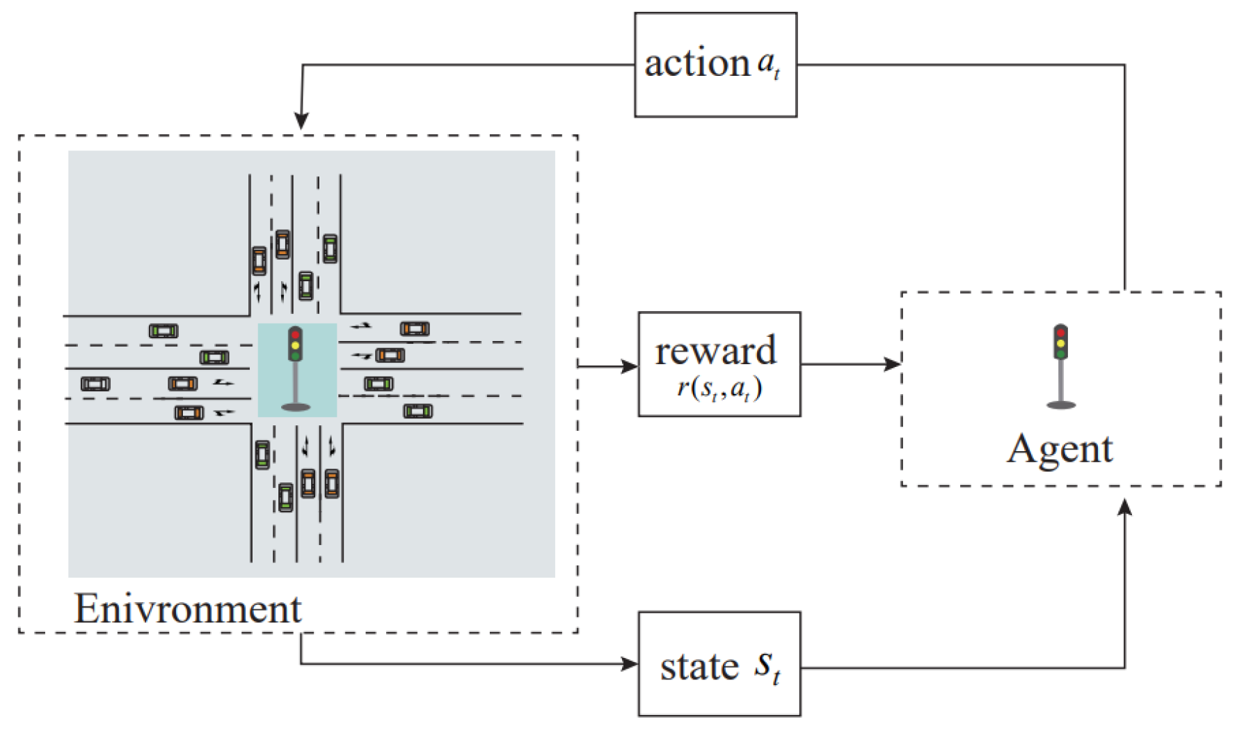
The classic Markov Decision Process (MDP) is composed of a five-tuple: $<S,A,P,R,\gamma >$. Here, S represents the state space; A denotes the action space; P is the state transition probability function, expressed as $P:S\times A\to S$, representing the probability of transitioning to the next state $s^{\prime }$ after taking an action in a given state $s$; R is the reward function, expressed as $R:S\times A\times \to R$, indicating the feedback received after executing an action in a given state $s$; $\gamma$ is the discount factor, representing the degree to which recent feedback influences future rewards, with $\gamma \in [0,1]$. Intersection signal control, as a traffic management strategy, can optimize traffic flow and reduce congestion. By adjusting signal timing through an intelligent signal system, intersections can be managed flexibly according to real-time traffic flow, thereby optimizing intersection performance. When addressing the signal control problem, it can be regarded as an MDP.

In DRL-based traffic signal control, the agent is represented by the traffic signal lights, and the environment corresponds to the road traffic conditions. In the decision-making process, the agent uses the input state to select appropriate actions and receives rewards as feedback from the environment. By designing suitable algorithms for the agent and training it to interact with the environment, the system can optimize signal timing and enable the agent to autonomously learn eco-friendly control strategies. The overall framework is illustrated in Figure 1.

2.2. State Space

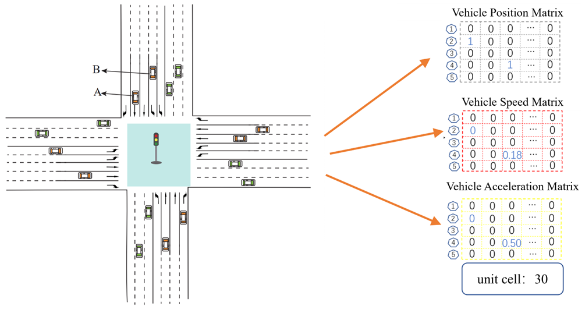
In urban intersections, the state refers to environmental variables that influence the agent’s decision-making process. Roadside equipment can use V2X technologies to obtain real-time vehicle information and make driving decisions based on the vehicle’s status and surrounding traffic environment. In this study, the state space designed for the agent includes information on vehicle position, speed, and acceleration. The Discrete Traffic State Encoding method is used to discretize the state space, thereby reducing its complexity and enhancing the expressiveness of the state information. The state space covers the approach lanes within 150 m of the stop line, divided into 5 m intervals, resulting in a state space matrix of size 3 × 19 × 30. To represent position information, elements 0 and 1 are used to indicate whether a vehicle is present at that position. When applying Min–Max normalization to vehicle speed and acceleration information, the calculation formula is as follows:

(1)

Normalization of vehicle instantaneous speed

$$V_{nor}={\displaystyle \frac{V-V_{min}}{V_{max}-V_{min}}}$$

(1)

where $V_{nor}$ represents the instantaneous normalized speed, which ranges from 0 to 1; $V$ is the instantaneous speed; $V_{min}$ is the minimum speed, set to 0.0 m/s; and $V_{max}$ is the maximum speed, determined by the road speed limit $V_{lim}$ and an overspeed factor $V_f$. The speed limit is set at 50 km/h. Considering that speeding occurs in real traffic conditions, a speeding factor of 1.2 was introduced so that the maximum speed is 60 km/h. The formula is as follows:

$$V_{max}=V_{lim}·V_f$$

(2)

(2)

Normalization of vehicle instantaneous acceleration

① When vehicle acceleration is positive, the formula is as follows:

$$Ac{c}_{nor}={\displaystyle \frac{Acc-Ac{c}_{min}}{Ac{c}_{max}-Ac{c}_{min}}}$$

(3)

where $Ac{c}_{nor}$ represents the instantaneous normalized acceleration; $Acc$ represents the instantaneous acceleration; $Ac{c}_{min}$ represents the minimum acceleration, set to 0.0 m/s²; and $Ac{c}_{max}$ represents the maximum acceleration, set to 2.6 m/s².

② When the vehicle acceleration is negative, the formula is as follows:

$$De{c}_{nor}={\displaystyle \frac{Dec-De{c}_{min}}{De{c}_{max}-De{c}_{min}}}$$

(4)

Here, $De{c}_{nor}$ represents the instantaneous normalized deceleration; $Dec$ represents the instantaneous deceleration; $De{c}_{min}$ represents the minimum deceleration, set to 0.0 m/s²; $De{c}_{max}$ represents the maximum deceleration, set to −9.0 m/s².

Taking the state space of the north entrance road as an example, the position information matrix corresponds to vehicles A and B at 0 m and 15 m from the stop line, and the processed velocity and acceleration information is entered into the matrix as illustrated in Figure 2.

2.3. Action Space

In this study, an adaptive signal phase switching strategy is chosen as the action space. Compared to fixed signal phases, the adaptive signal phases allow for more flexible decision-making by the agent. The action space is set to $A=\left\{\left.NSG,NSLG,EWG,EWLG\right\} \right.$, with phase actions selected as shown in

Table 1. Phase action selection.

Phase Number	Vehicle Travel Direction	Phase Illustration
1	$NSG$
2	$NSLG$
3	$EWG$
4	$EWLG$

, where right-turning vehicles are allowed to turn right under safe conditions.

To minimize disruptions from frequent phase changes, the maximum green light time is set to 50 s, with a minimum of 10 s, and the yellow light time is set to 3 s [19,22]. The agent has two types of actions to choose from: one is to extend the current phase’s green light duration by 5 s, denoted as $\Delta t=5$; the other is to switch to the next phase after the yellow light time has elapsed.

2.4. Reward Function

Deep reinforcement learning aims to maximize rewards. The agent learns a strategy based on the rewards obtained from each action taken to make better action decisions. The model’s reward function is established with a focus on reducing CO₂ emissions and improving intersection traffic efficiency.

(1)

Traffic efficiency

$$R_1=b_1{D}_{t-1}-D_t$$

(5)

where $D_t$ and $D_{t-1}$ represent the total waiting time at the intersection at time $t$ and $t-1$, respectively. Multiple experiments have shown that setting the weighting coefficient $b_1$ to 0.9 helps the agent better learn and optimize strategies.

(2)

Carbon emissions

$$R_2=b_2{E}_{t-1}-E_t$$

(6)

where $E_t$ and $E_{t-1}$ represent the total CO₂ emissions at the intersection at time $t$ and $t-1$, respectively, and $b_2$ is set to 0.9.

To make more accurate decisions based on vehicle CO₂ emissions, real-time speed and acceleration information are obtained using roadside sensors. The instantaneous carbon emissions of fuel vehicles are computed through the Vehicle Specific Power method (VSP), while the instantaneous carbon emissions of electric vehicles are computed from the perspective of energy conversion efficiency.

①

Instantaneous CO₂ emissions of conventional gasoline vehicles

Instantaneous energy consumption of gasoline vehicles is determined using the VSP method, known for its simplicity and wide applicability. As noted in the literature [44], the formula for VSP is as follows:

$$VSP=v\left(1.1a+9.81grade+0.132\right)+0.000302v^3$$

(7)

where $v$ and $a$ denote the instantaneous speed and acceleration of the vehicle, respectively, and $grade$ denotes the road gradient. Given that the study scenario involves urban intersections, we set $grade$ = 0, simplifying the calculation formula as follows:

$$VSP=v(1.1a+0.132)+0.000302v^3$$

(8)

According to the simplified formula, the calculation of VSP only requires the vehicle’s instantaneous speed and instantaneous acceleration. The accurate division of specific power (VSP) intervals is crucial for the precision of vehicle exhaust emission measurements. Frey [45] divided the VSP into 14 operational condition intervals, with the emission rate for each interval representing the average instantaneous emission rate of various pollutants. The instantaneous CO₂ emissions of a fuel-powered vehicle can be determined based on the CO₂ emission rates corresponding to different specific power intervals, as shown in

Table 2. Vehicle CO₂ emission rates for different VSP intervals.

Serial Number	Specific Power Interval (kw/t)	CO2 Emission Rate (g/s)	CO2 Emissions per Second
1	<−2	1.5437	1.5437
2	−2~0	1.6044	1.6044
3	0~1	1.1308	1.1308
4	1~4	2.3863	2.3863
5	4~7	3.2102	3.2102
6	7~10	3.9577	3.9577
7	10~13	4.7520	4.7520
8	13~16	5.3742	5.3742
9	16~19	5.9400	5.9400
10	19~23	6.4275	6.4275
11	23~28	7.0660	7.0660
12	28~33	7.6177	7.6177
13	33~39	8.3224	8.3224
14	≥39	8.4750	8.4750

.

②

Instantaneous CO₂ emissions of new energy electric-powered vehicles

From the perspective of energy conversion, the instantaneous electricity consumption of electric vehicles is converted into instantaneous CO₂ emissions using the national grid’s CO₂ emission factor. The formula for calculating the electricity consumed to charge electric vehicle batteries at time $t$ is as follows:

$$W_t={\displaystyle \frac{W_e}{{\eta }_{gb}}}$$

(9)

where $W_e$ represents the instantaneous total electricity consumption of electric vehicles; ${\eta }_{gb}$ represents the charging loss rate, set at 0.97; and $W_t$ represents the actual power consumption at the time $t$.

As per the Ministry of Environmental Protection Climate Directive [2023] No.43 [46], the CO₂ emission factor is specified as $0.5703 \mathrm{t}\mathrm{C}{\mathrm{O}}_2/\mathrm{M}\mathrm{W}\mathrm{h}$. The formula for calculating carbon emissions from electric vehicles is as follows:

$$W_c=W_t·0.5703$$

(10)

where $W_c$ represents the actual carbon emissions per second of the vehicle.

(3)

Comprehensive reward function

Combining both carbon emissions and traffic efficiency, the comprehensive reward function (Reward–CO2Reduction) is as follows:

$$R_{C{O}_2}=k_1(b_1{E}_{t-1}-E_t)+k_2(b_2{D}_{t-1}-D_t)$$

(11)

where $k_1$ and $k_2$ are weighted factors are determined by the mean queue length of vehicles at the intersection. The formula for calculating these weights is as follows:

$$k_1=\left\{\begin{array}{l}{e}^{-1.2({\displaystyle \frac{Queu{e}_{avg}}{Queu{e}_{std}}})}-0.2, Queu{e}_{avg}\le Queu{e}_{std}\\ e^{-1.2}-0.2, Queu{e}_{avg}>Queu{e}_{std}\end{array}\right.$$

(12)

$$k_2=\left\{\begin{array}{l}1.2-e^{-1.2({\displaystyle \frac{Queu{e}_{avg}}{Queu{e}_{std}}})}, Queu{e}_{avg}\le Queu{e}_{std}\\ 1.2-e^{-1.2}, Queu{e}_{avg}>Queu{e}_{std}\end{array}\right.$$

(13)

where $Queu{e}_{avg}$ represents the average number of vehicles in the queue for each lane, and $Queu{e}_{std}$ represents the average queue threshold. This threshold can be adjusted to modify the weights. In this study, considering that, when fuel-powered vehicles and electric vehicles mix, the carbon emissions of electric vehicles in an idling state are lower than those of traditional fuel-powered vehicles, the optimization effect of the carbon emission index is easily influenced by the current vehicle composition at the intersection. Therefore, it is necessary to dynamically adjust the weight coefficients of carbon emissions and waiting time, allowing the agent to find the optimal solution. After multiple experiments, the threshold is set to 3.

3. Methodology

3.1. DQN

Reinforcement learning is employed for agents to learn how to find the optimal set of actions in decision-making problems under uncertain environments. The agent achieves transitions between environmental states by taking actions at discrete time steps: when an action is executed, the environment produces a reward and transitions to a new state, formalized as a MDP. The agent’s actions are formalized as a policy π, which is represented by the value function $V^{\pi }$. The formula is as follows:

$$V^{\pi }(s)={\rm E}[\sum _{t=0}^{\infty }{\gamma }^{t}R(s_t,a_t)\left|s_0=s,s_t,a_t\right.]={{\rm E}}_{a\sim \pi (s)}[R(s,a)+\gamma {{\rm E}}_{s^{\prime }\sim {\rm P}(s,a)}{V}^{\pi }(s^{\prime })]$$

(14)

Here, $s_t\sim p(s_{t-1},a_{t-1})$ and $a_t\sim \pi (s_t)$, respectively, with the latter being the Bellman recursive equation. The optimal policy is derived by calculating Q-values for each state-action pair and applying the Bellman equation, then using a greedy strategy to choose the action with the highest Q-value.

$$Q*(s,a)={\rm E}[r+\gamma \underset{a^{\prime }}{max} Q*(s^{\prime },a^{\prime })\left|s,a\right.]$$

(15)

DQN [47] combines Q-learning with deep networks, with key techniques being experience replay and target networks:

• Setting up two neural networks can improve learning stability: one for determining actual values (main network) and one for predicting future values (target network). The target network is represented by a feedforward neural network consisting of three convolutional layers and two fully connected layers.
• A replay buffer D is set up to store experiences. Random sampling experiences for training can improve data efficiency and reduce the correlation between samples.

3.2. Rainbow DQN

Traditional DQN cannot handle environments with large continuous state-action pairs. Rainbow DQN [39], an advanced reinforcement learning algorithm, enhances the traditional DQN by integrating six major improvement methods: Double QL, Dueling Q-networks, Prioritized Experience Replay, Multi-step Learning, Distributional RL, and Noisy Nets, thereby improving model performance:

• Double DQN decouples value estimation and action selection between the targets to mitigate the overestimation bias in the primary Q-network.
• Prioritized Experience Replay samples experience with greater loss more frequently to accelerate training.
• Dueling Q-networks introduce dueling networks by modifying the DQN architecture to predict the advantages and value of states, respectively.
• Multi-step Learning uses multi-step targets instead of single-step targets to compute the temporal difference error, speeding up the convergence of $Q(s,a)$ values.
• Noisy Nets add normally distributed noise parameters to each weight in the fully connected layers, updating the weights through backpropagation. This replaces the standard greedy exploration strategy used in DQN with a noisy linear layer that includes noise streams.
• Distributional RL predicts $Q(s,a)$ values as distributions by minimizing Kullback–Leibner loss, offering deeper insights when evaluating specific states through the distributional Q function.

3.3. Rainbow DQN Algorithm Process

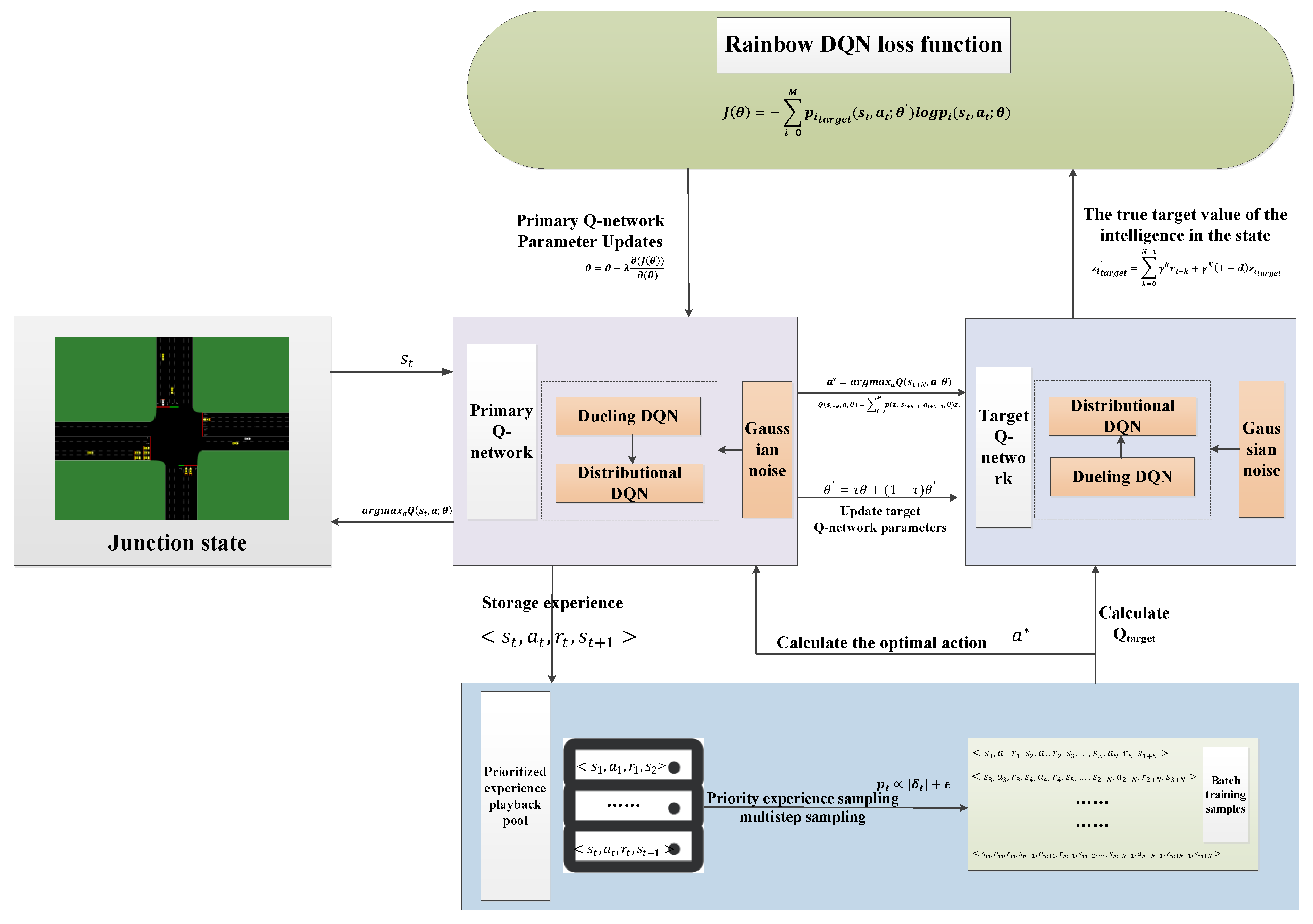
Figure 3 shows the framework of the intersection signal control algorithm based on Rainbow DQN_AM, which consists of two parts: the intersection signal control strategy and neural network parameter updates.

The Rainbow DQN intersection signal control algorithm is based on DQN [47], so its algorithmic flow closely resembles that of the DQN algorithm. The specific steps are as follows:

Step 1: parameter settings, including $\theta$—initialization of the main Q-network parameters; ${\theta }^{\prime }$—initialization of the target Q-network parameters; $D$—experience replay pool; $\gamma$—discount factor; $\tau$—smoothing coefficient; $\lambda$—learning rate of the main Q-network; $\epsilon$—exploration rate; $M$—maximum capacity of the experience replay pool; $B$—training batch size; $\mu$—target Q-network update frequency; $I$—number of iterations; $N$—total number of training episodes; and $T$—simulation episode time.

Step 2: initialize the experience replay pool with a capacity of M; initialize the Rainbow DQN main network $Q(s,a;\theta )$ and its corresponding parameters θ; initialize the target network $Q_{target}(s,a;{\theta }^{\prime })$ and its corresponding parameters ${\theta }^{\prime }$.

Step 3: start the iteration, generate the traffic scenario, and obtain the initial intersection environment state $s_0$.

Step 4: Generate a random probability value $r$. If $r<$ε, randomly select a control action for the traffic signal $a_t$. If $r>$ε, the network outputs a control action $a_t$ based on the current intersection environment state $s_{t+1}$, $a_t=\underset{a}{max}Q(s_t,a;\theta )$.

Step 5: Execute the action $a_t$, obtain the new intersection state $s_{t+1}$ and the corresponding reward $r_t$. Store the tuple $(s_t,a_t,r_t,s_{t+1},d)$ as a sample in the experience replay buffer, with the sample priority calculated based on the TD error $\left|\delta \right|$. If the experience buffer is full, delete the oldest sample record.

Step 6: Network update: The neural network parameters are updated using prioritized experience replay. After the parameters are updated, if the iteration count has not reached the predefined value, proceed to Step 4. Otherwise, proceed to Step 7. The process for updating the neural network parameters is as follows:

(1) The prioritized experience replay strategy is used to sample tuples $(s_t,a_t,r_t,s_{t+1},d)$ from the experience pool. It is important to note that, due to the multi-step learning strategy, samples from the current tuple to the next N steps in the future need to be collected.

(2) The optimal action $a*$ is calculated using the main Q-network in the Double DQN network, as shown in the following formula:

$$a*={argmax}_{a}Q(s_{t+N},a;\theta )$$

(16)

where $Q(s_{t+N},a;\theta )$ represents the expected value of the action $a$ taken by the main Q-network at the state $s_{t+N}$. The expected value of the main network is calculated through the distributional output of the Distributional DQN, as shown in the following formula:

$$Q\left(s_{t+N},a;\theta \right)={\sum }_{i=0}^{M}p(z_i|s_{t+N-1},a_{t+N-1};\theta )z_i$$

(17)

where $z_i$ represents the value of the $i$-th sample point; $p(z_i|s_{t+N-1},a_{t+N-1};\theta )$ denotes the probability of the $i$-th sample point when the main Q-network takes action $a_{t+N-1}$ at state $s_{t+N-1}$.

(3) The target Q-value distribution is computed using the target network, based on the multi-step learning strategy. The formula is as follows:

$${z_i}_{target}^{\prime }=\sum _{k=0}^{N-1}{\gamma }^k{r}_{t+k}+{\gamma }^N\left(1-d\right){z_i}_{target}$$

(18)

where ${z_i}_{target}$ is the Q-value distribution of the optimal action $a*$ from the target Q network, $\gamma$ is the discount factor, and ${z_i}_{target}^{\prime }$ represents the true target value of the agent at state $s_t$.

(4) The error between the true value distribution and the estimated value distribution is calculated using the cross-entropy loss function. The formula for the cross-entropy loss function is as follows:

$$J\left(\theta \right)=-\sum _{i=0}^M{p_i}_{target}(s_t,a_t;{\theta }^{\prime })log{p}_i(s_t,a_t;\theta )$$

(19)

where ${p_i}_{target}(s_t,a_t;{\theta }^{\prime })$ represents the true probability of the $i$-th sample point computed by the target network, and the predicted probability $p_i(s_t,a_t;\theta )$ is jointly computed using Dueling DQN and Distributional DQN.

(5) Update the parameters of the main network: the parameters $\theta$ of the main network are updated by minimizing the loss function $J(\theta )$ using stochastic gradient descent.

(6) Periodically synchronize and update the target network: The parameters of the target Q network are updated using delayed and soft update strategies to mitigate the overestimation problem in the main network. The update formula is as follows:

$${\theta }^{\prime }=\tau \theta +(1-\tau ){\theta }^{\prime }$$

(20)

In the equation, $\tau$ is the smoothing factor, representing the degree to which the main Q network’s parameters influence the target network.

Step 7: end of the process.

3.4. Algorithm Improvements Based on Rainbow DQN

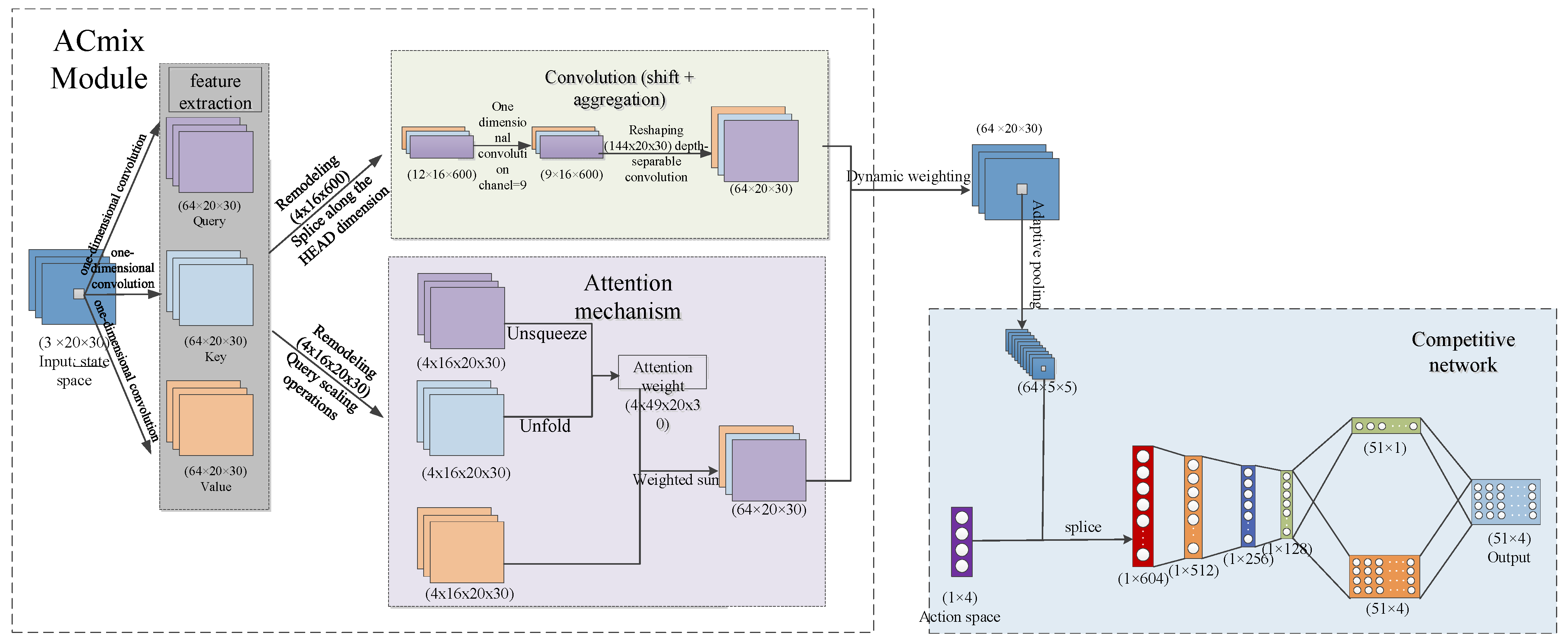
Based on the Rainbow DQN framework, we designed an efficient and comprehensive Rainbow DQN_AM model by introducing the ACmix module to address the discretized state space. Traditional CNN models excel at extracting local data features but struggle to capture sufficient global information. On the other hand, while LSTM models can capture temporal patterns, they lack effective spatial modeling capabilities. In intersection signal optimization, traffic flow is complex and dynamically changing, which requires models to have strong state information capturing abilities. Moreover, real-time signal optimization demands high computational efficiency to quickly process large amounts of state data. Combining sufficient state information extraction with rapid computation efficiency helps to enhance the model’s decision-making capabilities. Pan [43] explored the relationship between self-attention mechanisms and convolution and proposed the ACmix module, which integrates both. This module retains the advantages of convolutional layers, such as parameter sharing, sparse interactions, and multi-channel processing, allowing it to efficiently learn features, reduce computational load, and enhance the model’s expressiveness. Additionally, by incorporating the self-attention mechanism, the ACmix module can handle long-range dependencies and global information, enabling a more comprehensive capture of global features in intersection traffic flow. The integration of these two modules compensates for CNN’s limitations in capturing global features while maintaining computational efficiency, thereby improving the model’s performance in complex traffic flow environments. The network structure is shown in Figure 4.

The pseudocode for the improved Rainbow DQN Algorithm 1 is as follows:

Algorithm 1. Rainbow DQN algorithm

Input: Parameters

1: For $e\in \left\{\left.1,2,3,\dots ,N\right\}\right.$ do; 2:      Initialize the intersection road network environment $s_0$; 3:      for $t\in \left\{\left.1,2,\dots ,T\right\}\right.$ do; 4:           Observe the intersection road network environment $s_t$, Select action $a_t$ based on the greedy policy and noisy network. Execute action $a_t$, obtain new state $s_{t+1}$, and receive a reward $r_t$; 5:           Store the tuple $(s_t,a_t,r_t,s_{t+1},d)$ as an experienced sample in the experience replay buffer $D$; 6:           If $\left|D\right|>M$ exceeds capacity, delete the sample with the lowest priority; 7:           Sample $(s,a,r,s^{\prime },d)$ batch samples of size $B$ from the experience replay buffer $D$ using a prioritized experience replay strategy; 8:           for each transition $(s,a,r,s^{\prime },d)$ do. Primary Q-network determines the optimal action $a*=\mathit{argmax} Q (s_{t+N},a;\theta )$; 9:                 Compute the target value $z_{i_{\mathit{target}}}^{\prime }={\sum }_{k=0}^{N-1}{\gamma }^k{r}_{t+k}+{\gamma }^N(1-d)z_{i_{\mathit{target}}}$; 10:                 Determine the target value distribution $p_{i_{\mathit{target}}}$ based on the target value; 11:                 Update parameters $\theta$ using the cross-entropy loss function; 12:                 $J(\theta )=-{\sum }_{i=0}^M{p}_{i_{\mathit{target}}}(s,a;{\theta }^{\prime })\mathit{log} p_i(s_t,a_t;\theta )$; 13:                 Update the sample priorities in the experience replay buffer; 14:                 At every $I$ step, update the target network parameters ${\theta }^{\prime }=\tau \theta +(1-\tau ){\theta }^{\prime }$. 15:           end 16:      end 17: end

4. Experiment and Results

4.1. Simulation Setup

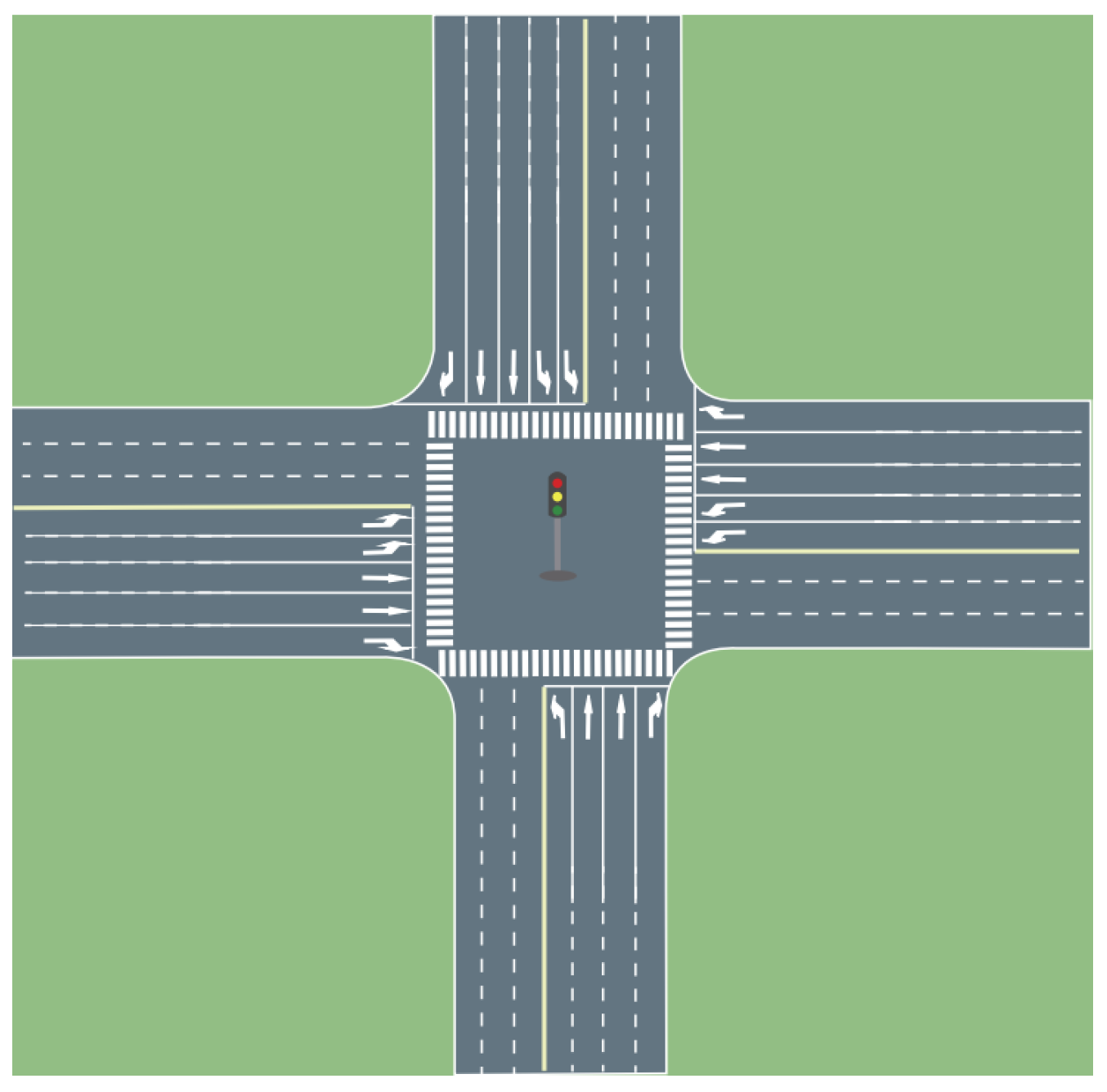
The LiZhou South Road—South City Road intersection in Jinhua City was chosen as the study site, and a simulation model was built in the SUMO simulation software (1.19.0). The intersection’s approach length is 400 m, with a speed limit of 50 km/h and a lane width of 3.75 m. The vehicle length is 5 m. The vehicle-following model adopted is the IDM, with a maximum acceleration of 2.6 m/s² [35], a maximum deceleration of −4.5 m/s² [19], a minimum safe following distance of 7.26 m [48,49], and a minimum stopping distance of 2.5 m [22]. The road structure of the simulated intersection is shown in Figure 5.

The signal timing data for the LiZouth Road—South City Road intersection in Jinhua City was collected. The actual signal cycle for the intersection is 179 s, with a yellow light duration of 3 s. Right-turning vehicles at this intersection are not controlled by the traffic signals. The specific phase distribution is shown in Figure 6.

The collected actual traffic flow data during peak hours is 4576 pcu/h, and the vehicle turning ratios at the intersection are shown in

Table 3. Vehicle turning ratios for each approach at the intersection.

	Straight-Through Ratio (%)	Left-Turn Ratio (%)	Right-Turn Ratio (%)
East Approach	10.29	4.56	5.03
West Approach	17.03	6.28	5.07
South Approach	14.16	4.09	4.56
North Approach	17.64	4.90	6.39

.

Considering the traffic flow characteristics during the morning and evening peak hours on urban roads, the traffic volume during peak periods often exhibits extreme fluctuations, where the flow quickly increases within a short period, maintains a peak state, and then sharply decreases. The Weibull distribution is well suited for capturing the significant fluctuations, extreme values, and nonlinear characteristics of peak traffic, making it ideal for simulating traffic distribution during peak hours. Therefore, traffic volume is generated based on the Weibull distribution. The simulation duration is set to 2 h, based on the collected traffic volume data, and the parameters of the probability distribution function are configured according to the method in reference [35]. The probability density function is as follows:

$$f(x;\lambda ,\alpha )=\left\{\begin{array}{l}{\displaystyle \frac{\alpha }{\lambda }}({\displaystyle \frac{x}{\lambda }}{)}^{\alpha -1}{e}^{-({\displaystyle \frac{x}{\lambda }}{)}^{\alpha }},x\ge 0\\ 0,x<0\end{array}\right.$$

(21)

Here, $\lambda$ is the scale parameter set to 1, and $\alpha$ is the shape parameter set to 2.

4.2. Comparison Experiment

(1) A comparison was conducted using D3QN, DQN, actual signal timing, Webster signal timing, actuated signal timing, and the Rainbow DQN algorithm-based signal timing. Among them, Webster signal timing and actuated signal timing are both traditional methods for signal optimization. For comparison, we selected two mainstream reinforcement learning models: DQN and D3QN. The DQN model serves as the foundational model for Rainbow DQN, while D3QN has garnered significant attention and is considered representative [50,51]. The DQN model configuration is based on the approach in [47], with the addition of a CNN module. The model setup and modules used in the D3QN model follow the configuration described in [35].

The actual signal timing is shown in Figure 6, and the key parameter settings for Webster signal timing and actuated signal timing are provided in

Table 4. Signal timing parameter settings for the control group.

Control Method	Parameters/Phases	Parameter Value (s)
Webster signal timing	East–West Straight	7
	East–West Left Turn	7
	North–South Straight	8
	North–South Left Turn	4
	Yellow Light Duration	4
actuated signal timing	Minimum Duration	5
	Maximum Duration	50

. The Webster signal timing parameters are calculated based on the actual intersection’s road network structure, traffic volume, and phase distribution to determine the optimal fixed signal timing. The actuated signal timing is based on the Webster signal timing parameters, with the maximum and minimum durations set according to [19]. The hyperparameters required for the DQN and D3QN algorithms are consistent with those used in Rainbow DQN.

To further validate the effectiveness of the reward function, a comparative reward function, Reward–Wait Time, was established. The calculation formula is as follows:

$$R_T=k_3{D}_{t-1}-D_t$$

(22)

where $D_t$ and $D_{t-1}$ represent the total vehicle waiting time at the intersection’s entry lane at time $t$ and $t-1$, respectively; $k_3$ is set to 0.9.

In summary, the experimental groups and control groups are set up as shown in

Table 5. Control group experimental design.

Control Method	Reinforcement Learning Method	Reward Function
Rainbow DQN_AM-CO2Reduction	Rainbow DQN_AM	Reward–CO2Reduction
Rainbow DQN_AM-Time		Reward–Wait Time
DQN-CO2Reduction	DQN	Reward–CO2Reduction
D3QN-CO2Reduction	D3QN	Reward–CO2Reduction
actual signal timing	/	/
Webster signal timing	/	/
actuated signal timing	/	/

.

(2) Analyze the control impact of the model under different scenarios, including varying CO₂ emission factors for electric vehicles, different proportions of electric vehicles, varying traffic volumes, and considering the penetration rate of autonomous vehicles.

4.3. Experimental Assumptions

(1) Roadside equipment can obtain real-time vehicle information through vehicular wireless communication technology (V2X). Communication delays and information errors are not considered.

(2) The study focuses only on passenger cars, ignoring the impact of vehicle size. From the perspective of vehicle power type, vehicles are categorized into two types: gasoline-powered and electric vehicles.

(3) All vehicles are equipped with the same devices, with the only difference being their power sources. Given the instability of start–stop devices in the current traffic environment [52,53], the impact of these devices on the model results is neglected.

(4) According to the 2023 Global Electric Vehicle Outlook [54], the current mix of gasoline and electric vehicles in traffic is set at 71% and 29%, respectively.

(5) The impact of pedestrians, non-motorized vehicles, and weather conditions on the road system is not considered [55].

(6) The study scenario is an urban intersection with a flat road surface, where factors such as slope have a negligible effect on the VSP-based power model [49].

4.4. Training Process

The Rainbow DQN_AM algorithm uses the Adam optimizer in combination with gradient descent for training. In each iteration, the batch size is set to 64. The number of epochs is set to 2880 simulation steps per epoch, and the model is trained for 100 epochs using real traffic flow data. The main hyperparameters of the algorithm are listed in

Table 6. Main hyperparameter of Rainbow DQN_AM.

Hyperparameters	Value
learning rate $\eta$	0.001
discount factor $\gamma$	0.99
batch size B	64
initial exploration probability ${\epsilon }_i$	0.99
final exploration probability ${\epsilon }_f$	0.01
[minimum value Zmin, maximum value Zmax]	−500,100
number of intervals	51
experience replay capacity M	200,000
multi-step learning steps	3
noisy network standard deviation	0.1
target network update frequency $\mu$	100
smoothing coefficient $\tau$	0.005

, with values referenced from [39]. The learning rate $\eta$, discount factor $\gamma$, and replay experience capacity M are determined through experimental tuning.

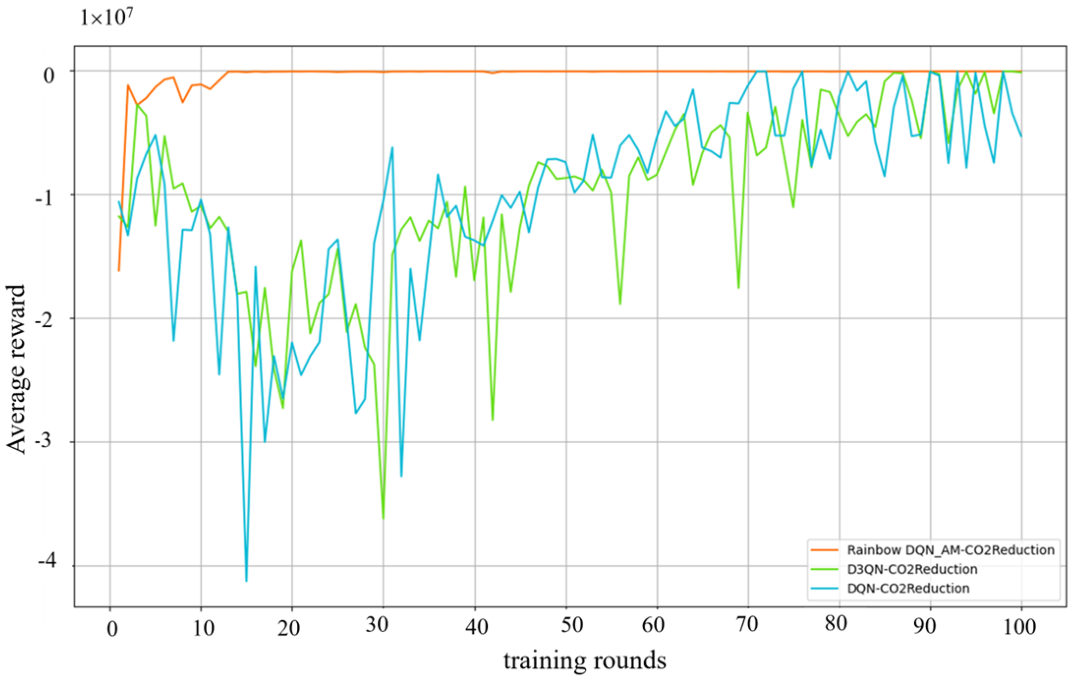
The network parameters from the training cycle with the highest average reward value were selected for model validation. Specifically, the parameters from the 92nd, 99th, and 71st generations were chosen for the Rainbow DQN_AM, D3QN, and DQN algorithms. As shown in Figure 7, the average reward values for the models indicate that the Rainbow DQN_AM algorithm exhibits the highest learning efficiency and fastest convergence, stabilizing after 14 generations. In contrast, the average reward curves for the DQN and D3QN algorithms show significant fluctuations. From the 5th to the 20th generation, the reward values drop sharply, and from the 20th to the 70th generation, the reward values fluctuate and rise but tend towards zero. Overall, the reward curves for these algorithms remain lower than that of the Rainbow DQN_AM algorithm.

4.5. Training Results

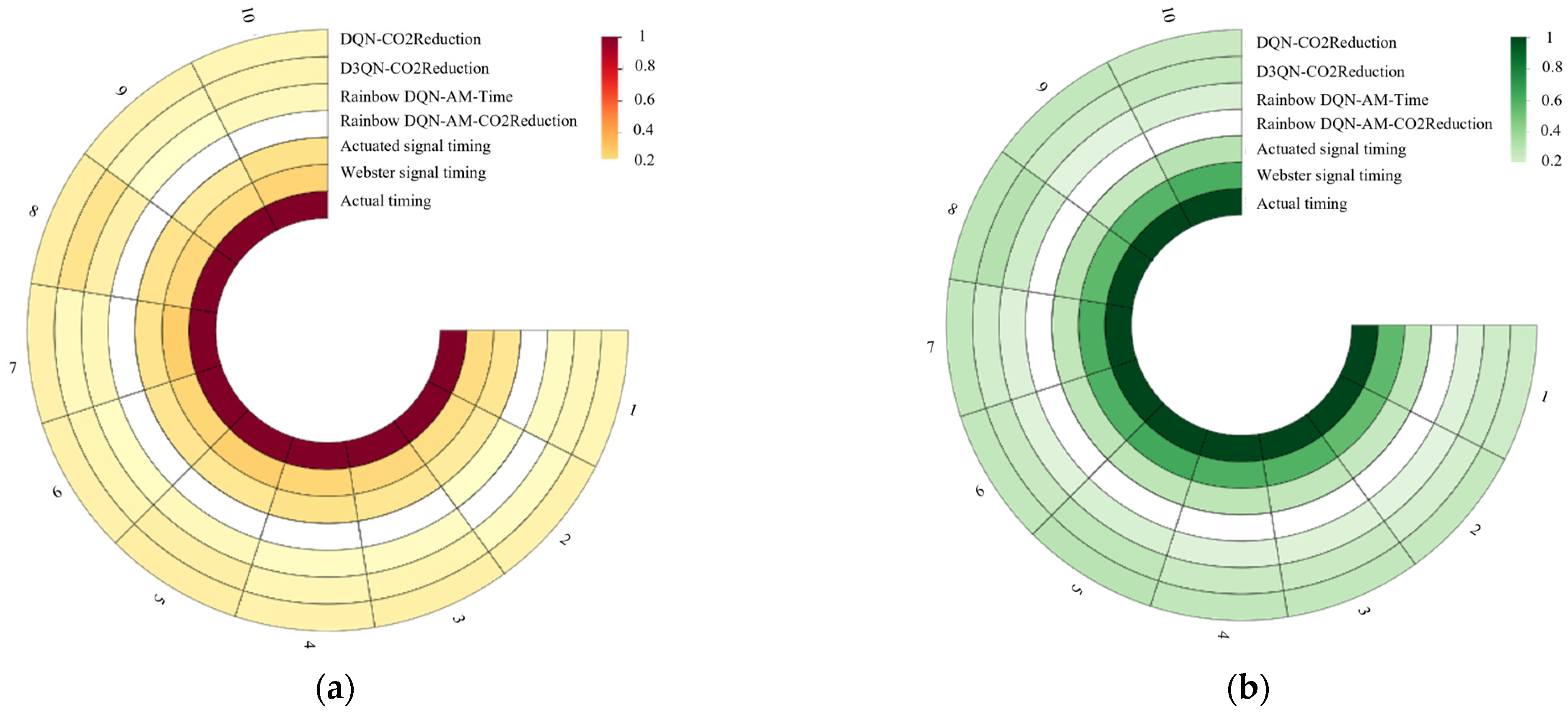
Using peak hour traffic data (4576 pcu/h) and the collected real traffic flow vehicle turn ratios, 10 sets of test traffic flows were randomly generated. The validity of the proposed signal control scheme was confirmed by assessing the average CO₂ emissions and vehicle waiting times throughout the simulation period.

Figure 8 shows a comparison of average vehicle CO₂ emissions and average waiting times. Min–Max normalization was applied to both metrics, and the results are presented as a heatmap. Each ring in the heatmap represents the optimization effectiveness of a signal control scheme, with lighter colors indicating better optimization results. Figure 8a shows the results for average vehicle waiting time. Compared to traditional signal control methods and actual signal timing, the DRL-based signal control methods provided better optimization for average vehicle waiting time at intersections. Among these, the Rainbow DQN_AM-CO2Reduction scheme performed the best, only slightly outperformed by the Rainbow DQN_AM_Time scheme in the second round of testing. Figure 8b displays the optimization effects on average vehicle CO₂ emissions. Similar to the results in the left figure, deep reinforcement learning control schemes generally outperformed traditional signal control algorithms across all test rounds. Furthermore, the Rainbow DQN_AM-CO2Reduction scheme consistently showed the best CO₂ reduction effects across all 10 test rounds. The results indicate that the two schemes using the Rainbow DQN_AM algorithm outperform the deep reinforcement learning schemes using D3QN and DQN.

A statistical significance analysis was conducted on the results for two indicators: average vehicle waiting time and average CO₂ emissions across different models. The Rainbow DQN_AM-CO2Reduction algorithm represents the optimized result, while the others serve as control groups. Data from 10 sets of traffic flow were used to perform an analysis of variance (ANOVA) to compare the indicator values from the control groups and the Rainbow DQN_AM-CO2Reduction algorithm. The results, shown in

Table 7. Statistical significance analysis of optimization indicators.

Control Method	Average Waiting Time	Average CO2 Emissions
	p-Value	p-Value
Actual signal timing	0.002	0.000
Webster signal timing	0.000	0.000
Actuated signal timing	0.000	0.000
Rainbow DQN_AM-Time	0.003	0.000
DQN-CO2 Reduction	0.000	0.000
D3QN-CO2 Reduction	0.000	0.000

, demonstrate that there are significant differences between the control group models and the proposed model in both average waiting time and average CO₂ emissions, with p-values less than 0.05. This indicates that the optimization effects of the model are statistically significant and representative.

To analyze the optimization degree of different schemes and the model’s robustness under real traffic conditions, box plots of the average vehicle waiting time and average CO₂ emissions are shown in Figure 9. Figure 9a shows that the average waiting time for vehicles for the Rainbow DQN_AM-CO2Reduction signal control scheme is 19.30 s. This represents reductions in 7.48%, 14.50%, and 27.58% compared with the Rainbow DQN_AM-Time scheme, the D3QN-CO2Reduction scheme, and the actuated signal timing scheme, respectively. Compared to the actual timing scheme, the reduction is as high as 57.95%. As shown in Figure 9b, the average CO₂ emissions per vehicle for the Rainbow DQN_AM-CO2Reduction scheme are only 190.33 g, which is 4.37%, 6.40%, and 7.34% lower than the Rainbow DQN_AM-Time scheme, the D3QN-CO2Reduction scheme, and the actuated signal timing scheme, respectively. In a scenario where electric vehicles account for 29% of the traffic, the average CO₂ emissions are optimized to a lesser extent than the average waiting time due to the low-emission nature of the electric vehicles themselves. Additionally, the Rainbow DQN_AM-CO2Reduction scheme shows standard deviations of 0.56 for average vehicle waiting time and 1.06 for average CO₂ emissions, significantly outperforming the Rainbow DQN_AM-Time scheme, which uses the same algorithm but with a different reward function. These results indicate that a reward function considering both waiting time and CO₂ emissions helps the agent learn a more reliable control strategy.

By analyzing the data on average waiting time and average CO₂ emissions, it is evident that in the simulation scenario using real traffic flow data, the proposed Rainbow DQN_AM-CO2Reduction model demonstrates clear superiority. Compared to the DQN and D3QN models, it reduces average waiting time by approximately 17.16% and 14.22%, respectively, and decreases average CO₂ emissions by about 6.94% and 6.39%.

To provide a comprehensive comparative analysis of the model, the results of this study are critically compared with those of related literature. Given that reinforcement learning models are influenced by various factors such as state space and reward functions, which can lead to differences in outcomes, we selected a study [35] as a comparison due to its similarities in state space, reward function, and other aspects with the proposed model. The model in [35] considers a mixed traffic scenario with Connected and Autonomous Vehicles (CAVs) and Human-driven Vehicles (HVs), using a D3QN framework with a CNN module. The state space includes vehicle position, speed, and acceleration, while the reward function considers average vehicle waiting time and CO₂ emissions with fixed weight parameters. A comparison of the optimization results between the proposed model and the model in [35], in relation to the optimization of signal timing with actuated signal control, is shown in

Table 8. Comparison of model optimization levels.

	Rainbow DQN_AM-CO2Reduction	D3QN_CNN
Average waiting time	27.58%	12%
Average CO2 emissions	7.34%	3.5%

. It is evident that, in the scenario based on real traffic data, the proposed model outperforms the D3QN_CNN model in terms of optimization. This suggests that the Rainbow DQN algorithm, as an integrated model, demonstrates superior performance in real-time signal optimization compared with the D3QN algorithm. Furthermore, the ACmix module introduced in this study enhances the model’s processing capabilities more effectively than the CNN module used in [35]. Additionally, compared with the fixed weighting of the reward function in [35], the dynamic adjustment of the queue length coefficient in the proposed model also contributes to the improved optimization performance. However, it is important to note that there are still some differences between the intersection scale, entry lane configuration, and traffic data used in [35] and those in this study. Furthermore, the mixed traffic scenario in [35] focusing on CAVs and HVs differs from the mixed traffic scenario with gasoline and electric vehicles in this study. Therefore, this comparison serves only as a reference.

4.6. Comparative Analysis of Different CO₂ Emission Factors for Electric Vehicles and Electric Vehicle Proportions

With the gradual development of electric vehicles (EVs), the proportion of EVs is expected to change in the future. At the same time, the CO₂ emission factors for electric vehicles published by the government vary annually. This section explores the model performance under different CO₂ emission factors for electric vehicles and varying proportions of electric vehicles, based on real traffic flow data.

4.6.1. Comparison Analysis Under Different CO₂ Emission Factors for Electric Vehicles

Due to the uncertainty in the future changes in CO₂ emission factors, this section selects the CO₂ emission factors for the years 2021, 2022, and 2023, as published by the Ministry of Ecology and Environment of China, to analyze their impact on the model results. 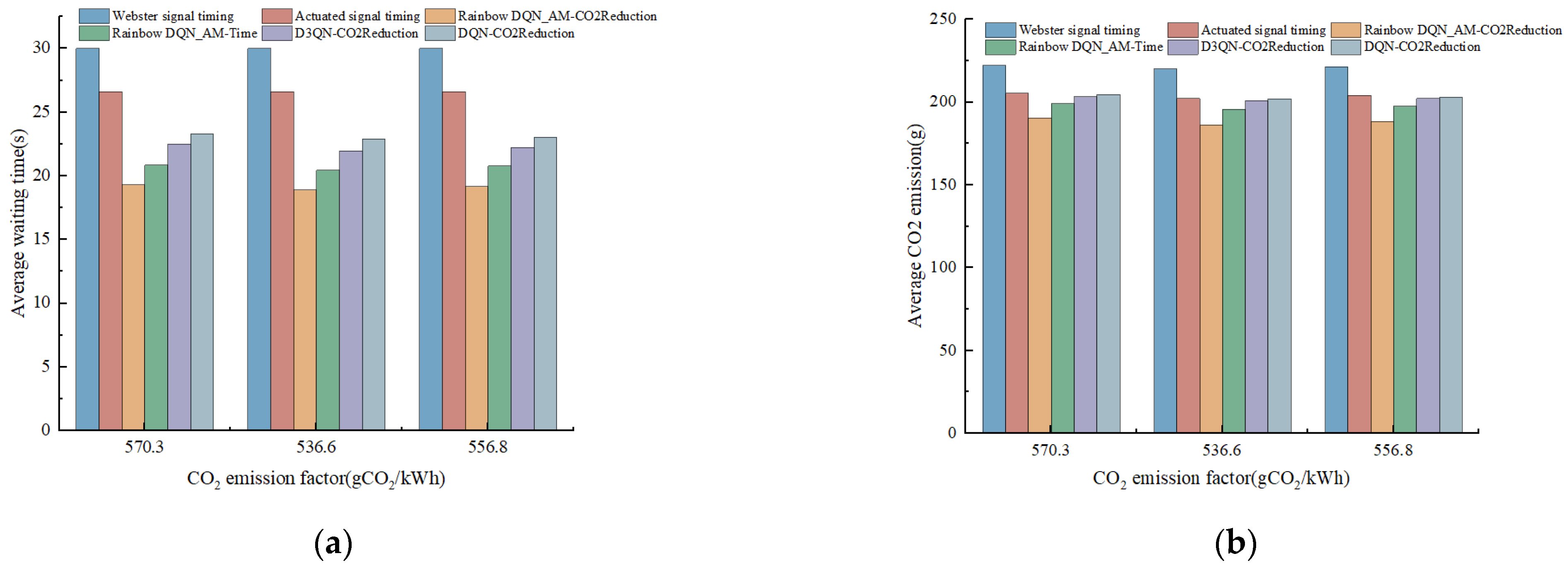The ratio of fuel vehicles to electric vehicles remains consistent with the assumptions, and the corresponding CO₂ emission factors are 556.8 g CO₂/kWh, 536.6 g CO₂/kWh, and 570.3 g CO₂/kWh, respectively. The changes in average vehicle waiting time and average CO₂ emissions under different CO₂ emission factors are shown in Figure 10. It can be clearly observed that, with variations in the CO₂ emission factor, there is no significant change in vehicle average waiting time, and the change in average CO₂ emissions is also relatively small. When the CO₂ emission factor is at its lowest value of 536.6 g CO₂/kWh, the Rainbow DQN-based optimization scheme shows the largest change in average CO₂ emissions, with variations reaching 3.46 g and 2.69 g, respectively. However, overall, there is no significant change. The average waiting time only changes by 0.3 s. This may be because, in the scenario where the proportion of electric vehicles is only 29%, changing the CO₂ emission factor has little impact on the vehicle’s average waiting time, and the change in CO₂ emissions is also minor. Furthermore, the logic of the reward function in this study involves dynamically weighting the differences in vehicle CO₂ emissions and waiting times between two consecutive time steps. When only the CO₂ emission factor for electric vehicles is altered, the relative differences between the two time steps are relatively small, so the reward function has little effect, and no significant change is observed.

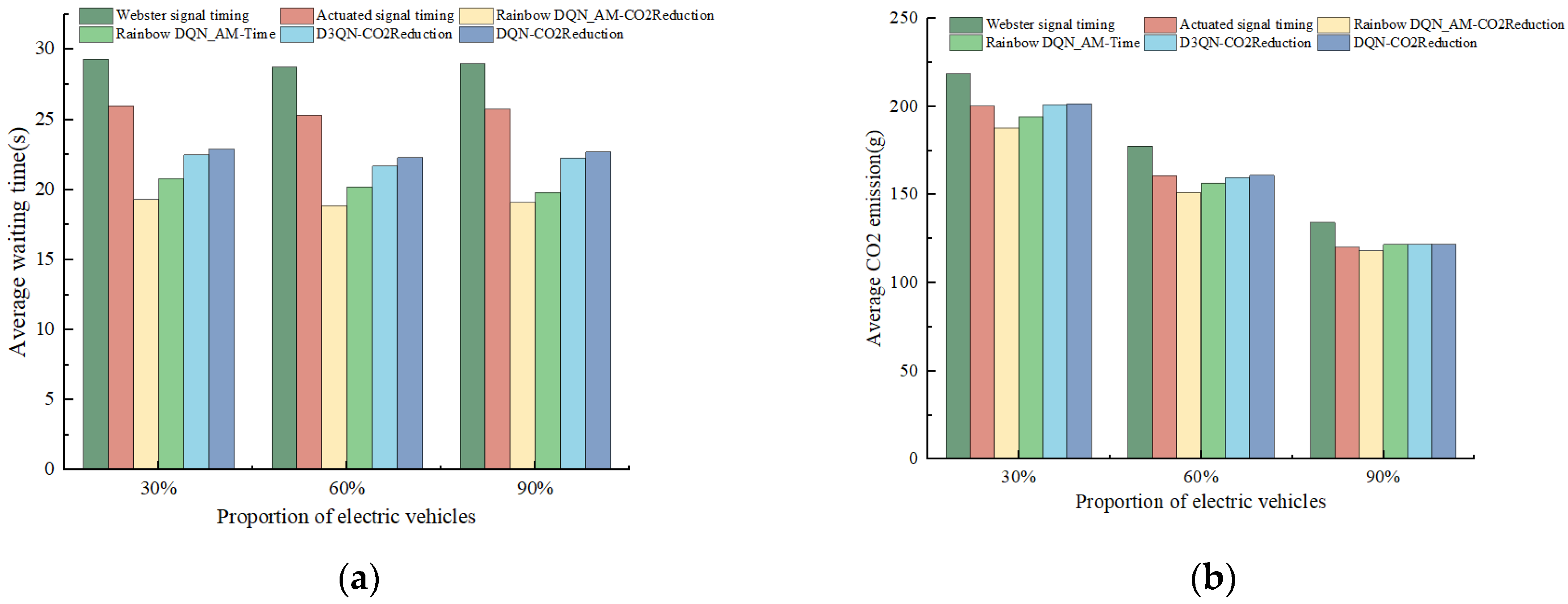
4.6.2. Comparison Analysis Under Different Proportions of Electric Vehicles

The proportion of electric vehicles was set to 30%, 60%, and 90% to explore the impact on the model’s optimization performance. The corresponding results for average vehicle waiting time and average CO₂ emissions are shown in Figure 11.

As shown in Figure 11a, the average waiting time for vehicles under different optimization schemes fluctuates as the proportion of electric vehicles increases. At 30% and 60% electric vehicle penetration, the Rainbow DQN_AM-CO2Reduction scheme reduces the average waiting time by more than 15% compared with the actuated signal timing. However, as the proportion of electric vehicles rises to 90%, the optimization effect of the proposed reward function weakens. The Rainbow DQN_AM-Time scheme, which focuses solely on the waiting time, maintains stable optimization performance. Additionally, due to the faster acceleration of electric vehicles, waiting times are reduced to some extent. Despite this, under the same reward function, the Rainbow DQN_AM-CO2Reduction method still achieves a more than 10% reduction in average waiting time compared with the DQN and D3QN models. As shown in Figure 11b, the increase in the proportion of electric vehicles leads to a natural decline in CO₂ emissions at the intersection. When the proportion of electric vehicles is 30%, 60%, and 90%, the corresponding average CO₂ emissions for the Rainbow DQN_AM-CO2Reduction scheme are 188.1 g, 151.44 g, and 118.3 g, respectively. As the proportion of electric vehicles increases, the optimization effect of the proposed scheme gradually weakens. At medium and low proportions, the scheme can reduce average CO₂ emissions by 4% to 7% compared with the actuated signal timing, but at a 90% electric vehicle proportion, the reduction is only about 2%. It is noteworthy that when the proportion of electric vehicles reaches 90%, the average CO₂ emissions from the D3QN-CO2Reduction and DQN-CO2Reduction optimization schemes show no significant difference compared with the actuated signal timing. This is because electric vehicles release much lower CO₂ emissions during idling, acceleration, and deceleration than conventional gasoline vehicles. At high electric vehicle proportions, the CO₂ emissions at the intersection are already at a low level, so the potential for further optimization is reduced.

4.7. Analysis of Experimental Outcomes Under Varying Traffic Volumes

Taking into account the significant variation in traffic flow at different times of the day on urban roads, this study not only validates the optimization effect of the model during peak hours but also compares and analyzes the performance of the intersection signal control strategy under three traffic intensities: 2400 pcu/h, 3600 pcu/h, and 4800 pcu/h. These traffic intensities correspond to vehicle arrival rates of 40 pcu/min, 60 pcu/min, and 80 pcu/min, respectively, simulating off-peak traffic conditions. By adjusting the green signal duration to 3 s and the yellow light duration to 2 s, the system can more effectively respond to varying traffic flow conditions.

As depicted in

Table 9. Average vehicle waiting time for different traffic intensities.

Control Method	Average Waiting Time (s)
	2400 pcu/h	3600 pcu/h	4800 pcu/h
Webster signal timing	13.51	20.51	35.91
Actuated signal timing	10.89	18.34	39.26
DQN-CO2Reduction	7.73	10.11	21.09
D3QN-CO2Reduction	4.85	7.45	22.70
Rainbow DQN_AM-Time	4.87	7.69	13.99
Rainbow DQN_AM-CO2Reduction	4.38	6.88	11.46

, the average vehicle waiting time increases with traffic flow, with the actuated signal timing scheme experiencing the greatest rise and the Rainbow DQN_AM-based scheme showing the least. The Rainbow DQN_AM-CO2Reduction scheme achieves the optimal optimization effect under all three traffic intensities, with waiting times of 4.38 s, 6.88 s, and 11.46 s, respectively. At traffic volumes of 2400 pcu/h and 3600 pcu/h, the D3QN-CO2Reduction scheme performs better than the Rainbow DQN_AM-Time scheme, with waiting times of 4.85 s and 7.45 s, respectively. At the highest traffic intensity, the optimization effectiveness of the timing schemes using the DQN and D3QN algorithms significantly declines, while the scheme based on the Rainbow DQN_AM algorithm demonstrates better robustness. Furthermore, the proposed scheme in this paper demonstrates the best optimization performance under high traffic intensity, reducing average waiting times by 18.08%, 45.66%, and 68.09% compared with the Rainbow DQN_AM-Time, DQN-CO2Reduction, and Webster signal timing schemes, respectively.

As shown in

Table 10. Average vehicle CO₂ emissions at different traffic intensities.

Control Method	Average CO2 Emissions (g)
	2400 pcu/h	3600 pcu/h	4800 pcu/h
Webster signal timing	190.55	200.30	218.26
Actuated signal timing	188.18	198.14	221.13
DQN-CO2Reduction	182.78	190.12	213.93
D3QN-CO2Reduction	178.28	183.12	212.01
Rainbow DQN_AM-Time	178.65	186.26	204.85
Rainbow DQN_AM-CO2Reduction	175.18	180.53	192.02

, the average vehicle CO₂ emissions increase overall with rising traffic flow. Consistent with the trend in vehicle waiting time, the Rainbow DQN_AM-CO2Reduction scheme achieves the best optimization results for average vehicle CO₂ emissions across all three traffic intensities, with values of 175.18 g, 180.53 g, and 192.02 g, respectively. In the 2400 pcu/h and 3600 pcu/h scenarios, the proposed scheme reduces CO₂ emissions by 1.73% and 1.41%, respectively, compared with the next best scheme, D3QN_CO2Reduction. In the 4800 pcu/h scenario, emissions are reduced by 6.26% compared with the next best scheme, Rainbow DQN_AM-Time. In medium and low traffic intensity scenarios, the optimization performance of the D3QN-CO2Reduction and DQN-CO2Reduction models, which are based on the same reward function, is inferior to that of the Rainbow DQN_AM-CO2Reduction scheme. As traffic intensity increases, the performance gap in model optimization widens further. Under high traffic intensity, the proposed model reduces average CO₂ emissions by 9.42% and 13.16% compared with D3QN-CO2Reduction and actuated signal timing schemes, respectively.

Under different traffic volume conditions, the Rainbow DQN_AM-CO2Reduction model demonstrated significant advantages in both the algorithm and reward function compared with classical DRL algorithms and reward functions. This confirmed its effectiveness in reducing the average vehicle waiting time and average CO₂ emissions at signalized intersections under mixed traffic conditions.

4.8. Analysis of Results Considering Different Autonomous Vehicle Penetration Rates

With the rapid development of autonomous driving technology, the proportion of autonomous vehicles in future transportation systems is expected to gradually increase. This trend will impact traffic flow characteristics, carbon emissions, and traffic efficiency. Therefore, it is necessary to analyze and compare the optimization effects of signal control schemes under different autonomous vehicle penetration rates.

Table 11. Current market penetration rate of vehicles.

	Human-Driven Vehicle	L2 Autonomous Connected Vehicle
fuel-powered vehicle (%)	51.4	19.6
electric vehicle (%)	13.7	15.3

presents global autonomous vehicle penetration rate data for 2023, and the market penetration rate of autonomous vehicles is expected to continue to rise in the future [54]. Based on this, this study assumes that the growth in autonomous vehicle market penetration will come primarily from autonomous electric vehicles, while the share of other vehicle types will decrease. A traffic flow of 4576 pcu/h is set, with manually driven vehicles modeled using the IDM model and autonomous vehicles modeled using the CACC model. Mixed traffic flows with 75%, 50%, and 25% connected vehicle penetration rates are randomly generated for testing. Additionally, the optimization effects of various signal control schemes are compared under two non-mixed traffic flow conditions: 100% and 0% penetration rates.

To accurately illustrate the performance differences of signal control schemes under varying penetration rates, Figure 12 shows that traditional signal control schemes, such as Webster and actuated signal control, perform less effectively in terms of average vehicle waiting time optimization in mixed traffic environments compared with non-mixed traffic environments. This is because, in mixed traffic conditions, especially under low penetration rates, connected autonomous vehicles cannot form an effective collaborative driving environment. In contrast, the proposed scheme in this study demonstrates more stable control strategies in mixed traffic environments. As the penetration rate increases, the average vehicle waiting time decreases. Specifically, at a 50% penetration rate, the average waiting time is 19.63 s, which is 6.35% lower compared with the scheme with the same algorithm but a different reward function, 14.20% lower compared with the scheme with the same reward function but a different algorithm, and 25.78% lower compared with the actuated signal control scheme.

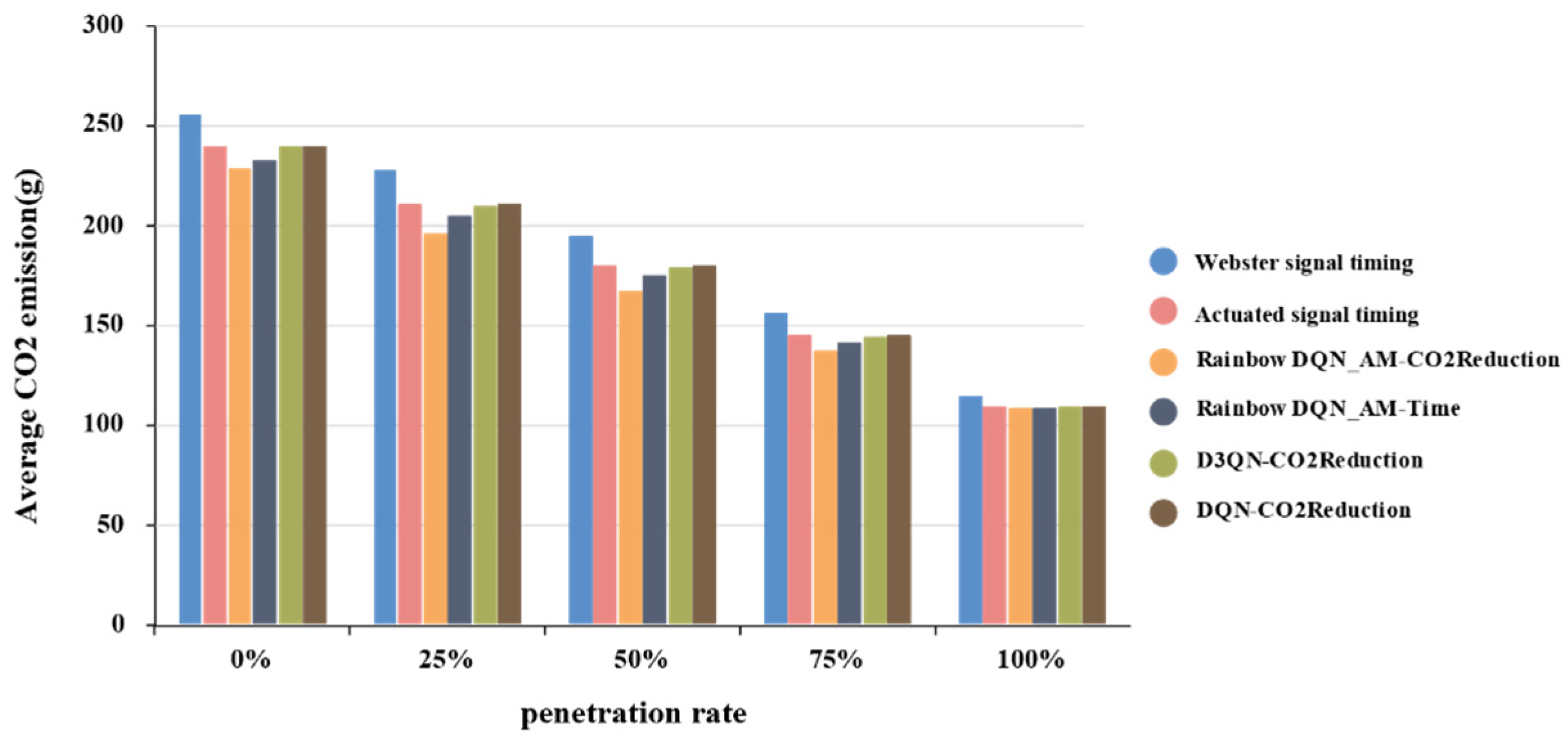
Figure 13 shows the trend of average vehicle CO₂ emissions under different penetration rates. Similar to Figure 12, the proposed optimization scheme performs best at a 50% penetration rate, where the average vehicle CO₂ emissions are 167 g. Compared to the Rainbow DQN_AM-Time scheme, D3QN-CO2Reduction, and the actuated signal timing scheme, emissions are reduced by 4.58%, 6.60%, and 6.97%, respectively. This is because, in a mixed-traffic environment, connected autonomous vehicles require frequent acceleration and deceleration, and other control schemes fail to learn the correct strategies effectively. It is noteworthy that at a 100% penetration rate, the CO₂ emissions component in the reward function is smaller, and thus, the performance difference between the proposed scheme and the Rainbow DQN_AM-Time scheme is not significant.

5. Discussion, Conclusions, and Limitations

5.1. Discussion

This study focuses on the mixed traffic scenario of gasoline vehicles and electric vehicles, aiming to propose an intersection signal timing optimization strategy based on deep reinforcement learning (Rainbow DQN) to improve intersection vehicle throughput and reduce CO₂ emissions.

Theoretically, this study utilizes the state-of-the-art Q-learning model, Rainbow DQN, providing a novel theoretical framework for optimizing traffic signal timing. Considering the increasing proportion of electric vehicles in real-world scenarios, this study fills the gap in existing literature by addressing the mixed traffic scenario involving both electric and gasoline vehicles. It incorporates the emission differences between gasoline and electric vehicles, selects appropriate carbon emission models, and designs a multi-objective reward function considering both traffic efficiency and CO₂ emissions. Additionally, the introduction of the ACmix module, which combines convolutional and self-attention mechanisms, enhances the model’s computational efficiency and expressive power. This also provides insights into mitigating the high computational and decision-making costs of real-time optimization while improving the potential application of reinforcement learning algorithms in complex traffic signal control problems.

In addition, by applying reinforcement learning algorithms to real-time traffic signal optimization, this study significantly improved traffic throughput and reduced CO₂ emissions through the dynamic adjustment of intersection signals. This provides an efficient, low-carbon, and intelligent optimization solution for intersection signal timing, offering valuable practical insights for urban traffic management. Through SUMO simulations, the optimization effects of the model were analyzed under different electric vehicle proportions and traffic volumes. In scenarios with a high proportion of electric vehicles, the optimization effect of the model weakened, and the performance of the DQN and D3QN models was lower than that of the conventional traffic signal control. This finding provides useful guidance for urban traffic managers in formulating strategies and further promotes the development of low-carbon cities, reducing traffic emissions. However, the model still needs to be validated in real-world traffic scenarios, and further consideration of the computational power required by the model is necessary to assess its applicability under real traffic conditions, providing stronger data support for broader future applications.

5.2. Conclusions and Limitations

This paper is based on the Rainbow DQN algorithm and utilizes the Reward–CO2 Reduction function for training to optimize intersection signal timing. The conclusions are as follows:

(1) Utilizing Rainbow DQN to explore real-time optimization of signal timing, the introduction of the Acmix module and self-attention mechanism significantly enhanced the model’s computational efficiency and performance. To facilitate efficient learning of signal control strategies by the agent, vehicle acceleration was incorporated into the state space modeling. The action space was defined based on variable phase sequences, while the reward function was formulated according to the average vehicle waiting time and CO₂ emissions. The calculation of CO₂ emissions at the intersection takes into account both the specific power model for fuel vehicles and the energy conversion model for electric vehicles, making it more reflective of real-world conditions.

(2) The model was validated using actual road intersection data, demonstrating the significant superiority of the Rainbow DQN_AM algorithm compared with signal timing based on DQN and D3QN algorithms. This also verified the effectiveness of the Reward-CO2 Reduction reward function. The proposed scheme reduces average vehicle waiting time by 7.48% and average CO₂ emissions by 4.37% compared with the Rainbow DQN_AM-Time scheme. It also achieves a reduction of approximately 27.58% in vehicle waiting time and about 7.34% in average CO₂ emissions compared with the actuated signal timing scheme.

(3) The impact of different CO₂ emission factors of electric vehicles on the model is not significant. As the proportion of electric vehicles increases, the optimization effect of the proposed reward function in this study decreases. At medium and low proportions of electric vehicles, compared with the actuated signal timing, the Rainbow DQN_AM-CO2Reduction method can reduce the average waiting time by more than 15% and decrease the average CO₂ emissions by 4% to 7%. Under varying traffic intensities, the Rainbow DQN_AM-CO2Reduction method adjusts its control strategy according to the traffic flow, reducing CO₂ emissions at the intersection and improving traffic efficiency. In the 3600 pcu/h traffic volume scenario, the proposed method shows the best optimization effect, but as traffic volume increases, the optimization effect decreases to some extent.

This study does have certain limitations. First, the research focuses solely on passenger cars and does not account for other types of vehicles. Future studies could include different vehicle types and categorize them based on their size and characteristics in the state input. Additionally, the model’s state–space input only considers factors such as vehicle position, speed, and acceleration. Previous studies [56] have demonstrated the feasibility of incorporating turn signal information into the state space. In the future, this information could be encoded as one of the state inputs to enhance the model’s adaptability at different intersections. Second, the model validation is primarily based on traffic flow data generated in a simulation environment and does not fully account for the complexities of real-world traffic scenarios, such as extreme weather conditions, unexpected events (e.g., traffic accidents), or fluctuations in pedestrian density. These factors may affect the model’s performance in actual environments, and further real-world testing is needed for validation. Lastly, the training process of Rainbow DQN is highly dependent on computational resources, especially in large-scale traffic networks. This could pose significant real-time challenges during training and deployment. Therefore, future research should incorporate real-world traffic data to improve the model’s generalization capability and explore more efficient algorithms to meet the demands of real-time optimization.