Abstract
This article outlines the results of comparison methods for representing complex data based on a redundant basis using the L0 norm and analyses the method of a modified MFNN (minimum fuel neural network) and the sparse representation method for the complex-data SL0 (smoothed L0 norm), based on the smoothed L0 norm. The example of numerical modeling for determining the direction of arrival (DOA) of sources received by an equidistant antenna array (ULA—Uniform Linear Array) shows that the SL0 method ensures a high convergence rate. However, unlike the MFNN-like neural network method, it does not guarantee convergence to the correct solution.
1. Introduction
In signal analysis, the direction of arrival (DOA) describes the direction from which a propagating wave usually arrives, reaching the point where the sensor set is located. This set of sensors forms the so-called sensor matrix. The DOA estimation is a widely used method for estimating the location of objects, for example, in a road scene formed by an automobile radar using the phase difference between signals received by different antenna elements included in an equidistant linear array. For a sensor matrix in the form of a linear array of antenna elements, the angular resolution of the signals for classical processing methods is limited by the ratio of the array size to the wavelength. This means that it is not possible to improve the resolution without increasing the size of the array. In some cases, this may not be feasible. At present, there is a sufficient number of research devoted to theoretical studies of direction-of-arrival estimation methods, their implementation options, as well as an assessment of the efficiency of using the methods to solve applied problems. Common examples of the DOA estimation method are the Capon method and the beamforming algorithm using the fast Fourier transform (FFT) [1,2,3,4]. The orthogonality of the eigenvectors of the noise part and the control vectors are used in the MUSIC (multiple signal classification algorithm) [5] and the more efficient ESPRIT (estimation of the signal parameters via the rotational invariance technique) [6] for determining the DOA of targets.
The mentioned DOA estimation algorithms [1,2,3,4,5,6] are based on an overdetermined system. Therefore, they have low resistance to errors or failure of individual receiving channels in the ULA, which is a factor that significantly worsens the DOA estimation results. In addition, these algorithms are not suitable for cases of highly correlated signals, which are signals reflected from objects.
In contrast, DOA estimation methods based on CS (compressed sensing) methods use the spatial sparsity of targets and are more reliable.
To estimate the DOA of received signals based on the CS (compressed sensing) method, an algorithm was proposed [7], which uses a vector of measurements of one or more snapshots of the received signal. Finding a solution with a minimum L0 norm is a problem whose complexity rapidly increases with increasing problem dimensionality and in the presence of noise in the input data. A fairly effective approach to solving this problem is the BP (basis pursuit) method [8,9], which allows finding a solution with a minimum L1 norm (i.e., a solution , for which the value is minimal), but it is still not fast enough, and it does not allow the use of complex data. The above methods provide the decomposition of data into weight components of the dictionary, which is an optimization problem with a basis of the L1 norm with linear constraints. Extending it to the complex space ℂ, we obtain the following:
where —input data, —basis components, and —the matrix of the redundant dictionary. . The input data b can be represented as follow:
where —is the residual vector, or error vector, the result of approximating b by the basis functions from the dictionary D, and is the i-th weighting factor of the corresponding basis component.
The solution to the optimization problem can be obtained by minimizing the norm of the loss function:
where —p-the norm, in general, is p = 2 (norm L2) or p = 1 (norm L1).
For the occasion p = 0: . Thus, L0 is the number of non-zero elements in x.
For the occasion p = 1: . Norm L1 represents the sum of the absolute values of elements in x.
The main difficulty in using the algorithms [7,8,9] is that they require large computational costs and the regularization parameter, which is associated with the cost function, strongly depends on the noise variance. If the noise variance used for the corresponding parameter does not meet the real noise variance, the efficiency of DOA estimation of the corresponding methods is reduced significantly.
In [10,11,12,13,14,15,16,17], the SL0 algorithm is presented, which implements a very fast method for searching for a sparse solution to an indefinite system of linear equations, including for data belonging to a complex space. The SL0 algorithm implements an estimated solution based on approximating the discontinuous function of the L0 norm with an arbitrary continuous function. In this case, the solution can be obtained from the global maxima of the corresponding function and the gradient method with a step-by-step projection of the result onto the space of admissible vectors. This method requires fewer computations than solving the problem of minimizing the L1 norm and does not require the exact noise variance. However, this algorithm is sensitive to the choice of the initial values of the coefficients and does not guarantee convergence to the optimal solution. The variant proposed in [14] makes it possible to significantly reduce the problem dimension without degrading the performance. In [15], a new model for representing a sparse signal using the lower left diagonals of the covariance matrix is proposed, and it demonstrates high performance in DOA estimation. An improved SL0 algorithm which uses correlation matrices and several signal snapshots instead of one is given in [16]. For performing sparse reconstruction using a single snapshot, traditional methods are ineffective due to the many neighboring targets and low signal-to-noise ratio. In [18], the problem of ill-conditioning when applying SL0 to Doppler range-angle estimates for a MIMO radar was studied and an efficient approach for MIMO radars based on using SL0 for this type of estimates was presented. A method that improves the efficiency of Doppler range imaging for a noisy radar was also presented in [19].
2. Smoothed L0 Norm Algorithm
In [10,11,12], there is Algorithm 1 SL0 (smoothed L0 norm), which implements a very fast method for searching for a sparse solution to an under-determined system of linear equations, including for data belonging to a complex space. The SL0 algorithm implements an approximate solution based on the gradient method, with a step-by-step projection of the result onto the space of feasible vectors [10]:
where K >> L, A is the selected matrix of the redundant basis, x is the solution vector, σ, μ, and are coefficients determining the speed of convergence, and H is the Hermitian conjugation symbol.
| Algorithm 1: SL0 |
, |
This algorithm was compared in [10] with L1-magic, one of the fastest implementations of the linear programming method (LP), and another fast iterative Re-weighted least squares algorithm (IRLS), using FOCUSS. The simulation results presented in [10] demonstrate the following relative convergence times (for SL0, the convergence time is assumed to be 1), as shown in Table 1.

Table 1.
The relative ratios of convergence times for a signal vector length of 1000 and a number of basis functions of 400.
The results of Table 1, as reported in [10], show that SL0 operates at a speed that is two orders of magnitude higher than that of LP or FOCUS, while achieving higher MSE values. The change in the normalized convergence rate for various modifications of SL0 is not significant and varies between 0.5 and 1.
3. Modified MFNN Algorithm
Along with the methods mentioned above, the decomposition of data into weighted components can be represented as a so-called “fuel minimization” problem or MFNN (minimum fuel neural network), as presented in [20], and its modified version for complex-valued data, proposed by the authors [21]. Cosine functions are used as a dictionary in [20]. It is shown that in the field of real numbers, ℝ, the neural network described by the system of differential equations gives a solution that is globally stable according to Lyapunov and approaches the exact solution of the problem (1). Despite the interesting results obtained, this approach has not been thoroughly investigated to date. The MFNN algorithm is described in more detail in [20], which provides a theoretical justification for an approach based on solving differential equations. The modified MFNN algorithm provides a solution for complex-valued data using a neural network approach with a modified initialization function, as described in [21]. It was demonstrated that by altering the initialization function for a neural network proposed in the paper, complex-valued data could be successfully represented using complex-valued basis elements.
The Algorithm 2 modified MFNN implements a solution for complex-valued data based on the neural network method:
where A is the selected matrix of the redundant dictionary, x is the solution vector, b the given signal, and is the initialization function.
| Algorithm 2: modified MFNN |
where , |
In fact, the MFNN algorithm implements a direct representation of a system of nonlinear differential equations describing the development of the state of a multidimensional dynamic system in the space of basis functions and can be represented as shown in the Figure 1:
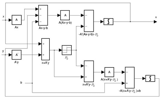
Figure 1.
Neural network architecture for MFNN.
As noted above, the SL0 method is sensitive to the choice of initial values of the coefficients and does not guarantee convergence to an optimal solution, unlike the modified MFNN.
4. Numerical Modeling
This section presents the results of a mathematical model of the modified MFNN algorithm and compares its effectiveness with the use of the SL0 algorithm. It solves the problem of determining the DOA for an equidistant antenna array with linear frequency modulation, where the input data are complex signals received by the elements of this array from several point sources. The received data can be represented as follows:
where γj = sin(θj) j = 1, 2, … J is the number of point external sources, d is the lattice element pitch normalized to the wavelength, m = 1,2, …M, M is the number of receiving elements of the antenna array, is the angular direction to the j-th source, is the amplitude of the j-th source, is the phase of the j-th source, and .
Then, the elements of the matrix, which comprise an overcomplete basic dictionary, can be represented as follows:
where , n = 1, 2, …, N is the dimension of the angular direction grid of the overcomplete basis dictionary, and m = 1, 2, …, M (M is the number of receiving elements of the antenna array).
To form the redundant basis A, a grid by angle N = 512 points was selected. The number of elements of the antenna array M = 16, and the step of the elements d = 0.5 wavelength. Numerical modeling was carried out using an Intel(R) Core (TM) i7-5960X CPU @ 3.00 GHz. and MATLAB ver. R2021b. Values from (7) were selected as elements of the excess basis matrix with N = 512, M = 16, and d = 0.5. The calculation results were output at the end of the cycle with a given number of iteration process steps, which varied from 250 to 10,000, with the total number of cycles being 100. The convergence rate of Algorithm 1 depends significantly on the coefficients that determine the parameters of the iteration process. The values of these coefficients were chosen as μ = 2.0 ÷ 3.9, = 0.3 ÷ 1.0 to ensure the maximum convergence rate without a loss of stability.
The following are the simulation results characterizing the accuracy and speed of Algorithm 2: Figure 2, Figure 3 and Figure 4 and Figure 5a,c,e,g and Algorithm 1: Figure 2, Figure 3, Figure 4 and Figure 5b,d,f,h. The simulation was carried out for various conditions. The number of point external sources with different amplitude and phase values varied from 1 to 6.
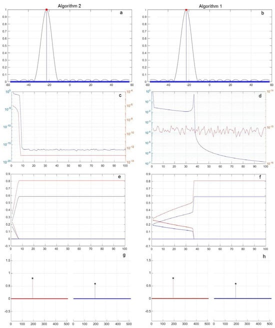
Figure 2.
Single-source 1, = −22.5°, with values of (a,b) |x|, (c,d) —blue, —red and (e,f) Re(x(t))—red, Im(x(t))—blue and (g,h) Re(x)—red, Im(x)—blue (*—shows the exact values). Algorithm 2—subfigure (a,c,e,g); Algorithm 1—subfigure (b,d,f,h).
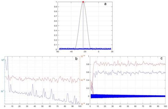
Figure 3.
Algorithm 1, single-source 1, = −22.5°, with values of (a) |x|, (b) —blue, —red and (c) Re(x(t))—red, Im(x(t))—blue, μ = 3.9, = 0.99.
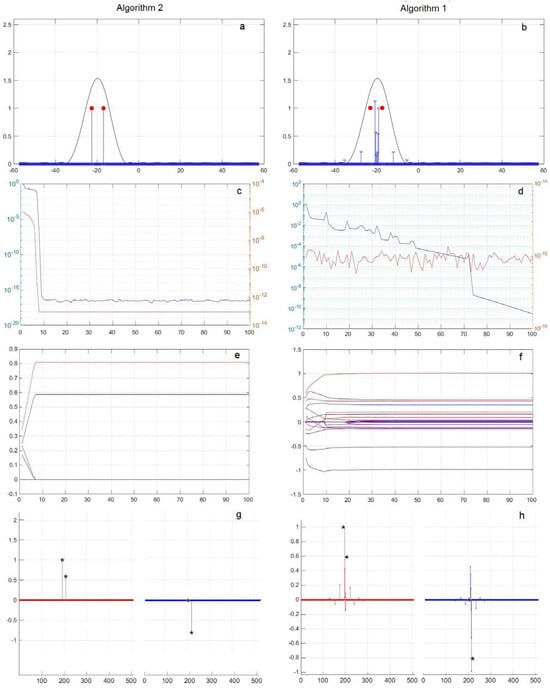
Figure 4.
Two sources of 1, = −22.5°, −16.88° and , with values of (a,b) |x|, (c,d) , and (e,f) Re(x(t))—red, Im(x(t))—blue and (g,h) Re(x)—red, Im(x)—blue (*—shows the exact values). Algorithm 2—subfigure (a,c,e,g); Algorithm 1—subfigure (b,d,f,h).
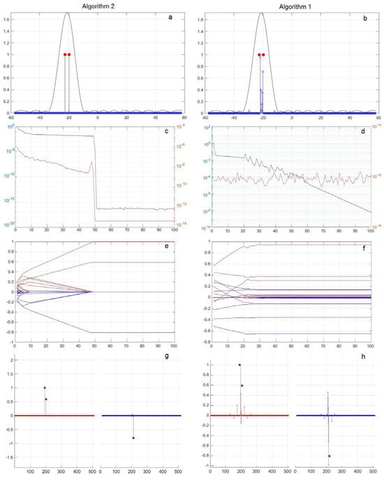
Figure 5.
Two sources of 1, = −22.5°, −19.69° and , with values of (a,b) |x|, (c,d) —blue, —red and (e,f) Re(x(t))—red, Im(x(t))—blue and (g,h) Re(x)—red, Im(x)—blue (*—shows the exact values). Algorithm 2—subfigure (a,c,e,g); Algorithm 1—subfigure (b,d,f,h).
In Figure 2a,b, Figure 3, Figure 4 and Figure 5a,b, the processing result (the vector of the coefficient modules |x| of the basis components upon completion of the algorithms) is shown in blue, and the result of standard processing using FFT with the Chebyshev weight distribution (a sidelobe level of −30 dB) is shown in black. The direction to the point sources, taking into account their amplitude, is depicted in red. The amplitude is plotted along the vertical axis, and the angular direction in degrees is represented along the horizontal axis.
Figure 2c,d, Figure 3, Figure 4 and Figure 5c,d show the maximum change for the current step of the solution process t of the vector elements of the basis components’ coefficients x. It is normalized from step to step to its value at the previous step and the current error in representing the input signals, which was defined as the loss function for norm L2. The current value is plotted along the vertical axis, and the current step number is plotted along the horizontal axis.
Figure 2e,f, Figure 3, Figure 4 and Figure 5e,f show the changes in the values of the real Re(x(t)) (red) and imaginary Im(x(t)) (blue) constituent elements of the vector x(t) of coefficients of the basis components by iteration steps. The current values of Re(x(t)) and Im(x(t)) are plotted along the vertical axis, and the current step number is shown along the horizontal axis.
Figure 2g,h, Figure 3, Figure 4 and Figure 5g,h outline the obtained values of the real (red) and imaginary (blue) components of the vector of coefficients of the basis components at the end of the iteration process and the values of the sources amplitudes (black asterisks). The values are plotted along the vertical axis, and the number of the basis components in the selected grid is depicted along the horizontal axis.
4.1. Single External Source
Below are the results of the numerical simulation of the operation of Algorithms 1 and 2 if there is the single point source with an amplitude of 1, an angle of arrival of θ1 = −22.5°, and phase . On the left, vertically, are the results for Algorithm 2 and on the right, vertically, are the results for Algorithm 2. For example, Figure 2b shows the plot for a FFT (black) and Algorithm 1 and resulting basis components coefficients |x| (blue).
It is evident from the obtained results that for the phase value , (i.e., provided that the phases of the basis functions (7) and the source phase do not coincide), the use of both algorithms leads to a solution with only one main non-zero basis coefficient, which corresponds to the amplitude, direction, and phase of the source, as shown in Figure 2a,b,g,h. In this case, the loss function characterizing the error in representing the input signals P becomes less than 10−13–10−15, and the rate of change of the coefficients for Algorithm 2 drops to 10−12, i.e., practically to zero. At the same time, the rate of change of the coefficients for Algorithm 1 decreases only to 10−7, which means that the process of changing the coefficients continues even after reaching the exact value.
For Algorithm 1, the result for μ = 2, = 1 converges after 40 cycles of 25,000 steps, while Algorithm 2 converges after 10 cycles of 6000 steps. Increasing μ to a value greater than 4 leads to a divergence of the iteration process for Algorithm 1. Intermediate values of μ from 2 to 4 allow for acceleration of the convergence, but require selecting α, and lead to a significant increase in random fluctuations in the coefficient values. They can be seen in Figure 3b, which shows the change in the iteration steps of (blue) and P(t) (red), and in Figure 3c, which shows the change in Re(x(t)) (red) and Im(x(t)) (blue), for μ = 3.9, α = 0.99.
Table 2 shows the number of excess basis coefficients, the value of which is normalized to the maximum value exceeding 0.1, 0.01, and 0.001.
Table 2.
Number of excess basis coefficients with a level exceeding 0.1, 0.01, and 0.001 for single source.
From the obtained results, it follows that for single sources, Algorithm 1 not only has no advantage over Algorithm 2 in terms of speed, but also, when using universal values μ = 2, α = 1, which ensure stability and small fluctuations in the coefficients, it turns out to be 17 times slower.
One more peculiarity of the coefficient behaviors for Algorithm 1 can be noted: shown in Figure 2d,f—the bulk of the coefficient values that differ from the exact solution very quickly become negligibly small, and during the same time, the loss function P also falls almost to zero, and the main coefficients stop changing much later. At the same time, for Algorithm 2, the changes in the coefficients and the loss function, as seen in Figure 2c,e, change in the same way and reach a stationary value simultaneously.
4.2. Two Separated External Sources
Next, Figure 4 (similar to Figure 2) show the results of a numerical simulation of the operation of Algorithms 1 and 2 if there are two point sources with an amplitude of 1, with angles of arrival of , , (angle difference 5.6 and the corresponding phase values for sources are = 0° and = −0.3π. On the left, vertically, are the values for Algorithm 2 and on the right, vertically, the values for Algorithm 1 are depicted. For example, Figure 4b shows the plot obtained for an FFT (black) and Algorithm 1 and resulting basis components coefficients |x| (blue).
In Figure 4a,b the angular directions in degrees are plotted along the horizontal axis (in the grid of angular directions of an overcomplete basic dictionary); along the vertical axis are the module values of the resulting basic components |x|, obtained as a result of processing using Algorithms 1 and 2. The modules of the radiation pattern values obtained using FFT (black) are shown in the same angular grid. The position of the point sources with the amplitudes and is represented by red dots.
From the result obtained in this case, the radiation pattern formed using FFT does not allow resolving sources at an angular distance equal to 5.38°.
The received results show that the use of Algorithm 2 leads to a solution with only two main non-zero basis coefficients, which correspond to the amplitude, direction, and phase of the sources, as shown in Figure 4a,h. In this case, the loss function characterizing the error in representing the input signals P(t) becomes less than 10−14, and the rate of change of the coefficients drops to 10−16, that is, actually to zero, and the results stop changing after 10 cycles of 6000 steps.
At the same time, for Algorithm 1, with the selected values μ = 2, α = 0.3, the rate of change of the coefficients 10−11, and the loss function P(t) becomes less than 10−14, as can be seen from Figure 4b,g, and the results themselves practically stop changing after 30 cycles of 6000 steps. Thus, for the case under consideration, the convergence time of Algorithm 2 is approximately three times less than for Algorithm 1. But, what is more important is that Algorithm 1 did not allow an exact solution to be found to the problem, which led to the appearance of a larger number of coefficients different from zero with their values of the amplitudes of angular directions and phases that do not coincide with the values for the two sources. In this case, the number of non-zero coefficients significantly exceeds 2.
Table 3 shows the number of excess basis coefficients, the value of which is normalized to the maximum value exceeding 0.1, 0.01 and 0.001.
Table 3.
Number of excess basis coefficients with a level exceeding 0.1, 0.01, and 0.001 for two separated sources.
From the obtained results, it follows that for paired sources, Algorithm 1 does not allow the finding of a global minimum in accordance with the L0 norm and gives a solution with a fairly significant error; this is unlike Algorithm 2, which gives two non-zero coefficients, which is the exact solution whose real and imaginary values coincide with the corresponding values of the sources.
4.3. The Case of Two Close Sources
Next, Figure 5 (similar to Figure 2 and Figure 4) show the results of a numerical simulation of the operation of Algorithms 1 and 2 if there are two point sources with an amplitude of 1, angles of arrival of , (angle difference 2.8 and the corresponding phase values for sources are = 0° and = −0.3π. On the left, vertically, are the values for Algorithm 2 and on the right, vertically, are the values for Algorithm 1. For example, Figure 5b shows the plot obtained for FFT (black) and Algorithm 1 and resulting basis components coefficients |x| (blue).
In Figure 5a,b the angular directions in degrees are plotted along the horizontal axis (in the grid of angular directions of an overcomplete basic dictionary); along the vertical axis are the module values of the resulting basic components |x|, obtained as a result of processing using Algorithms 1 and 2. The modules of the radiation pattern values obtained using FFT (black) are shown in the same angular grid. The position of the point sources with the amplitudes and is represented by red dots.
From the result received in this case, the radiation pattern formed using FFT does not allow resolving sources at an angular distance between them equal to 5.38°.
It is evident from the results that the use of Algorithm 2 leads to a solution with only two main non-zero basis coefficients, which correspond to the amplitude, direction, and phase of the sources, as shown in Figure 5a,h. In this case, the loss function characterizing the error in representing the input signals P(t) becomes less than 10−14, a and the rate of change of the coefficients drops to 10−16, that is, actually to zero, and the results stop changing after 50 cycles of 15,000 steps.
At the same time, for Algorithm 1, with the selected values of μ = 1.5, α = 0.3, the rate of change of the coefficients 10−9, and the loss function P(t) becomes less than 10−15, as can be seen from Figure 5b,g, and the results themselves practically stop changing after 30 cycles of 15,000 steps. Thus, for the case under consideration, the convergence time of Algorithm 2 is approximately three times less than for Algorithm 1. Algorithm 1, similar to the case in Section 4.3, did not allow an exact solution to be found to the problem, which led to the appearance of a larger number of non-zero coefficients with their own values of the amplitudes of angular directions and phases that do not coincide with the values for two sources. In this case, the number of non-zero coefficients significantly exceeds 2, and the angular shift of the two main coefficients was 0.50° and −0.25°, respectively.
Table 4 shows the number of excess basis coefficients, the value of which is normalized to the maximum value exceeding 0.1, 0.01 and 0.001.
Table 4.
Number of excess basis coefficients with a level exceeding 0.1, 0.01, and 0.001 for two close sources.
It follows from the obtained results that Algorithm 1 also does not allow the finding of a global minimum in accordance with the L0 norm for the paired close sources. This suggests a solution with a rather significant error; this is in contrast to Algorithm 2, which finds an exact solution with two non-zero coefficients, the real and imaginary values of which coincide with the corresponding values of the sources, while the speeds of the algorithms are close.
4.4. A Large Number of Sources
Next, Figure 6 (similar to Figure 2, Figure 4 and Figure 5) show the results of a numerical simulation of the operation of Algorithms 1 and 2 if there are six point sources with an amplitude of , an angles of arrival of , and the corresponding phase values for sources are . On the left, vertically, there are the values for Algorithm 2 and on the right, vertically, the values for Algorithm 12 are given. For example, Figure 5b shows the plot obtained for FFT (black) and Algorithm 1 and resulting basis components coefficients |x| (blue).
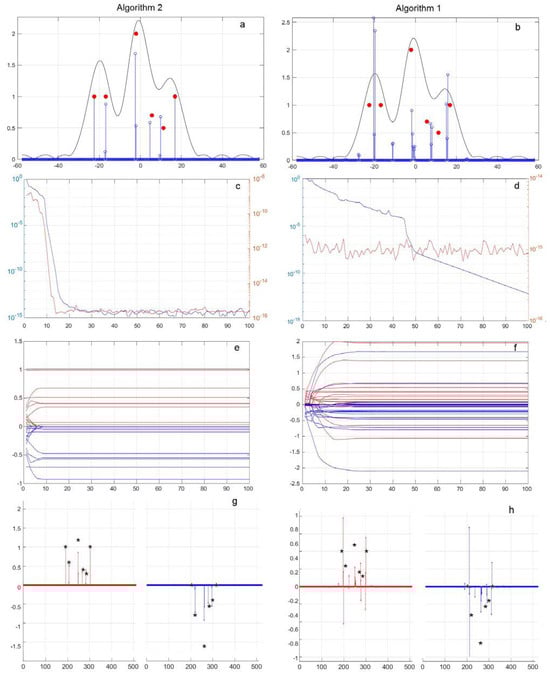
Figure 6.
Six sources with values of (a,b) |x|, (c,d) —blue, —red and (e,f) Re(x(t))—red, Im(x(t))—blue and (g,h) Re(x)—red, Im(x)—blue (*—shows the exact values). Algorithm 2—subfigure (a,c,e,g); Algorithm 1—subfigure (b,d,f,h).
In Figure 6a,b the angular directions in degrees are plotted along the horizontal axis (in the grid of angular directions of an overcomplete basic dictionary); along the vertical axis are the module values of the resulting basic components |x|, obtained as a result of processing using Algorithms 1 and 2. The modules of the radiation pattern values obtained using FFT (black) are shown in the same angular grid. The position of the point sources with the amplitudes is represented by red dots.
From the result obtained in this case, the radiation pattern formed using FFT does not allow resolving sources. Instead of the position corresponding to six sources on the FFT graph, only three peaks can be determined.
From the received results, it is clear that the use of Algorithm 2 leads to a solution with seven main non-zero basis coefficients, which are close in amplitude, direction, and phase to the corresponding values of the sources, as shown in Figure 5a,h. The loss function characterizing the error in representing the input signals P(t) becomes less than 10−16, and the rate of change of the coefficients drops 10−15, that is, actually to zero, and the results stop changing after 15 cycles of 300,000 steps.
At the same time, for Algorithm 1, with the selected values of μ = 1.5, α = 0.3, the rate of change of the coefficients decreases to 10−9, and the loss function P(t) becomes less than 10−15, as can be seen from Figure 6b,g, and the results themselves practically stop changing after 30 cycles of 70,000 steps. Thus, for the case under consideration, the convergence time of Algorithm 2 is approximately two times less than for Algorithm 1. However, Algorithm 1 did not allow an exact solution to be found to the problem, which led to the appearance of a larger number of non-zero coefficients with their own values of the amplitudes of angular directions and phases that do not coincide with the values for six sources. In this case, the number of non-zero coefficients significantly exceeds six, and the angular shift of the main coefficients varies from 3.50° to −0.5°.
Table 5 shows the number of excess basis coefficients, the value of which is normalized to the maximum value exceeding 0.1, 0.01, and 0.001.
Table 5.
Number of excess basis coefficients with a level exceeding 0.1, 0.01, and 0.001 for six close sources.
It follows from the obtained results that, for several sources, Algorithm 1 also does not allow the finding of a global minimum in accordance with the L0 norm. This gives a solution with a significant error, in contrast to Algorithm 2. Although this Algorithm also does not find an exact solution with six non-zero coefficients, the real and imaginary values of which coincide with the corresponding values of the sources; however, the deviations from the exact solution in directions do not exceed 0.5°, while the speeds of the algorithms are close.
5. Conclusions
This article considers the results of comparing two algorithms for representing data from the complex space based on an excess basis using the L1 norm. Algorithm 1 based on the sparse representation method for complex data SL0 (smoothed L0 norm), based on the smoothed L0 norm, and Algorithm 2 based on the method using a modified MFNN are analyzed. Using numerical modeling for determining the DOA and direction of sources received by an equidistant antenna array (ULA—Uniform Linear Array), it is shown that the solutions implemented in the form of Algorithm 1, based on the SL0 method, are dependent on the choice of the values of the coefficients μ, α. It should be underlined that the choice of universal optimal values of these coefficients is difficult. At the same time, the modified MFNN method allows for high accuracy in finding the optimal solution for different values of positions, amplitudes, phases, and the number of sources, and the convergence rate of the modified MFNN method implemented in the form of Algorithm 2 is in some cases higher than the convergence rate of the SL0 method. Thus, it can be concluded that algorithm 2 is preferable in terms of the stability and accuracy of the solution, and its convergence rate characteristics are close to those of Algorithm 1.
In subsequent studies, there is a plan to conduct a detailed analysis of the convergence rate and stability of the method, as well as an experimental study of its characteristics for data processing using dictionaries based on functions other than exponential ones.
Author Contributions
Methodology, N.V.P.; software, N.V.P. and I.A.K.; writing—original draft preparation, N.V.P. and A.Y.N.; writing—review and editing, N.V.P. and A.V.K. All authors have read and agreed to the published version of the manuscript.
Funding
This research was funded by the Ministry of Science and Higher Education of the Russian Federation within the framework of state assignment No. FZRR-2023-0008.
Institutional Review Board Statement
Not applicable.
Informed Consent Statement
Not applicable.
Data Availability Statement
The raw data supporting the conclusions of this article will be made available by the authors on request.
Conflicts of Interest
The authors declare no conflicts of interest.
References
- Li, Y.; Cichocki, A.; Amari, S.I. Sparse component analysis for blind source separation with less sensors than sources. In Proceedings of the ICA2003, Nara, Japan, 1–4 April 2003; pp. 89–94. [Google Scholar]
- Georgiev, P.G.; Theis, F.J.; Cichocki, A. Blind source separation and sparse component analysis for over-complete mix-tures. In Proceedings of the ICASSP’04, Montreal, QC, Canada, 17–21 May 2004; pp. 493–496. [Google Scholar]
- Gribonval, R.; Lesage, S. A survey of sparse component analysis for blind source separation: Principles, perspectives, and new challenges. In Proceedings of the ESANN’06, Bruges, Belgium, 26–28 April 2006; pp. 323–330. [Google Scholar]
- Mehrpooya, A.; Karbasi, S.M.; Nazari, M.; Abbasi, Z.; Nayebi, M.M. 3D inverse synthetic aperture radar image quality improvement using sparse signal representation. IET Radar Sonar Navig. 2023, 17, 388–407. [Google Scholar] [CrossRef]
- CandÁes, E.J.; Tao, T. Decoding by linear programming. IEEE Trans. Inf. Theory 2005, 51, 4203–4215. [Google Scholar] [CrossRef]
- Haardt, M.; Nossek, J.A. Simultaneous Schur Decomposition of Several Nonsymmetric Matrices to Achieve Automatic Pair-ing in Multidimensional Harmonic Retrieval Problems. IEEE Trans. Signal Process. 1998, 46, 161–169. [Google Scholar] [CrossRef]
- Donoho, D.L. For most large underdetermined systems of linear equations the minimal 𝓁1-norm solution is also the sparsest solution. Commun. Pure Appl. Math. 2006, 59, 797–829. [Google Scholar] [CrossRef]
- Malioutov, D.; Cetin, M.; Willsky, A. A sparse signal reconstruction perspective for source localization with sensor arrays. IEEE Trans. Signal Process. 2005, 53, 3010–3022. [Google Scholar] [CrossRef]
- Zhang, C.; Yin, Z.; Chen, X.; Xiao, M. Signal overcomplete representation and sparse decomposition based on re-dundant dictionaries. Chin. Sci. Bull. 2005, 50, 2672–2677. [Google Scholar] [CrossRef]
- Mohimani, H.; Babaie-Zadeh, M.; Jutten, C. A fast approach for overcomplete sparse decomposition based on smoothed ℓ0 norm. IEEE Trans. Signal Process 2008, 57, 289–301. [Google Scholar] [CrossRef]
- Mohimani, G.H.; Babaie-Zadeh, M.; Jutten, C. Complex-valued sparse representation based on smoothed l0 norm. In Proceedings of the IEEE International Conference on Acoustics, Speech and Signal Processing, Las Vegas, NV, USA, 31 March–4 April 2008; pp. 3881–3884. [Google Scholar] [CrossRef]
- Wang, L.; Yin, X.; Yue, H.; Xiang, J. A regularized weighted smoothed L0 norm minimization method for underdetermined blind source separation. Sensors 2018, 12, 4260. [Google Scholar] [CrossRef] [PubMed]
- Oxvig, C.S.; Pedersen, P.S.; Arildsen, T.; Larsen, T. Improving Smoothed l0 Norm in Compressive Sensing Using Adaptive Parameter Selection. Available online: https://arxiv.org/abs/1210.4277 (accessed on 10 October 2024).
- Xiang, J.; Yue, H.; Yin, X.; Wang, L. A New Smoothed L0 Regularization Approach for Sparse Signal Recovery. Math. Probl. Eng. 2019, 2019, 1978154. [Google Scholar] [CrossRef]
- Han, Y.; Wang, J. Adaptive beamforming based on compressed sensing with smoothed l0 norm. Int. J. Antennas Propag. 2015, 2015, 1–10. [Google Scholar]
- Cai, J.; Bao, D.; Li, P. DOA estimation via sparse recovering from the smoothed covariance vector. J. Syst. Eng. Electron. 2016, 27, 555–561. [Google Scholar] [CrossRef]
- Paik, J.W.; Lee, J.-H.; Hong, W. An Enhanced Smoothed L0-Norm Direction of Arrival Estimation Method Using Covariance Matrix. Sensors 2021, 21, 4403. [Google Scholar] [CrossRef]
- Chen, J.; Li, W.; Li, J.; Zhu, Y. Robust smoothed l0-norm based approach for MIMO radar target estimation. IET Radar So-Nar Navig. 2017, 11, 1170–1179. [Google Scholar] [CrossRef]
- Lu, X.; Gu, H.; Su, W. Noise radar range doppler imaging via 2D generalized smoothed-l0. Electron. Lett. 2021, 57, 448–450. [Google Scholar] [CrossRef]
- Wang, Z.S.; Cheung, J.Y.; Xia, Y.S.; Chen, J.D.Z. Minimum fuel neural networks and their applications to overcomplete signal representations. IEEE Trans. Circuits Syst. I Fund. Theory Appl. 2000, 47, 1146–1159. [Google Scholar] [CrossRef]
- Panokin, N.V.; Averin, A.V.; Kostin, I.A.; Karlovskiy, A.V.; Orelkina, D.I.; Nalivaiko, A.Y. Method for Sparse Representation of Complex Data Based on Overcomplete Basis, l1 Norm, and Neural MFNN-like Network. Appl. Sci. 2024, 14, 1959. [Google Scholar] [CrossRef]
Disclaimer/Publisher’s Note: The statements, opinions and data contained in all publications are solely those of the individual author(s) and contributor(s) and not of MDPI and/or the editor(s). MDPI and/or the editor(s) disclaim responsibility for any injury to people or property resulting from any ideas, methods, instructions or products referred to in the content. |
© 2025 by the authors. Licensee MDPI, Basel, Switzerland. This article is an open access article distributed under the terms and conditions of the Creative Commons Attribution (CC BY) license (https://creativecommons.org/licenses/by/4.0/).