Condition-Based Maintenance Decision-Making for Multi-Component Systems with Integrated Dynamic Bayesian Network and Proportional Hazards Model

Abstract

A condition-based maintenance decision-making framework for multi-component systems is proposed in this work by integrating dynamic Bayesian network (DBN) with proportional hazards model (PHM). The framework is designed to address the challenge of handling mixed failure types and complex failure dependencies, which often lead to inaccurate maintenance decisions in existing methods. In this integrated model, the DBN captures the failure evolution and both dynamic and static dependencies among components, while the PHM enhances the capability to characterize mixed failure interactions, thereby enabling the coverage of three common types of failure dependencies in multi-component systems. The model is formulated and solved using a finite-horizon Markov decision process (MDP), with the optimal maintenance strategy obtained by maximizing the total expected reward. Numerical case studies demonstrate the framework’s flexibility in handling mixed failures and complex dependencies, showing its potential to effectively support condition-based maintenance decision-making for complex multi-component systems.

1. Introduction

In modern industrial systems, unplanned downtime of critical equipment due to failures can result in significant economic losses and serious safety incidents. As a result, developing effective condition-based maintenance (CBM) strategies that balance system risk and maintenance costs has become a central focus in reliability engineering. Accurate maintenance decisions rely heavily on the precise assessment of system failure states. However, traditional single-component failure models and maintenance policies are often inadequate for multi-component systems commonly encountered in engineering practice. Moreover, the prevalence of failure dependencies, such as structural, stochastic, and economic dependencies [1,2], makes the assumption of component independence unrealistic, frequently leading to biased state estimation and suboptimal maintenance decisions. Thus, designing accurate and efficient maintenance strategies for multi-component systems remains a key challenge.

Existing research on maintenance decision-making for multi-component systems primarily addresses two issues: (1) capturing the failure states of individual components, and (2) quantifying failure dependencies among components. Component failures are generally classified as either discrete (hard failures) or degradation-based (soft failures), and are commonly modeled using failure rate functions, Markov processes, or other stochastic models [3,4]. To represent failure interactions, commonly used approaches include copula functions, proportional hazards models (PHM), and state-space models [5]. Copula functions are particularly suitable for capturing dependencies among multiple degrading components. For example, Xu [6] applied a copula to model stochastic dependence in a K-out-of-N system with degrading components and developed an optimized CBM strategy within a Markov decision process (MDP) framework. Similarly, Li [7] used a Nested Lévy copula to represent hierarchical stochastic dependencies in a four-component system and derived a corresponding maintenance policy.

The PHM incorporates covariate effects into the baseline hazard function, allowing for the representation of diverse and dynamic failure dependencies. Xu [8] extended the PHM to include state-dependent covariates, constructing a joint failure rate model for a two-component system and applying it to optimize gearbox bearing maintenance. Zhou [9] integrated a non-homogeneous Poisson process into the PHM covariates to support maintenance decisions for systems subject to competing dependent risks—minor and major failures. Hu [10] incorporated a degradation process as a time-varying covariate in the PHM to estimate the failure rate of a hard failure system, enabling online maintenance decisions based on remaining useful life distribution.

Bayesian Networks, as probabilistic graphical models, offer a flexible way to represent failure dependencies among components. Dynamic Bayesian networks (DBNs) can further capture time-varying dependencies, making them well-suited for reliability modeling and maintenance planning of multi-component systems [11,12,13,14]. Hu et al. [15] combined DBNs with Hazard and Operability analysis for opportunistic predictive maintenance planning. Cai et al. [16] used DBNs to compare perfect repair, imperfect repair, and preventive maintenance strategies for a subsea blowout preventer. Özgür-Ünlüakın [17] incorporated maintenance action nodes into a DBN to model stochastic, structural, and economic dependencies, and designed proactive maintenance policies for a thermal power plant. Faddoul [18] and Morato [19] integrated Bayesian networks with MDPs and used dynamic programming and decision trees to optimize maintenance and inspection policies.

As multi-component systems grow in structural and dependency complexity, recent research has trended toward incorporating more components and multiple dependency types. However, multivariate copulas are limited to representing a single type of joint distribution and struggle with mixed failure modes and dynamic dependencies. While PHMs accommodate dynamic covariates, they lack flexibility in modeling multiple coexisting dependency types across many components. DBNs naturally support scalable and dynamic dependency modeling, yet existing DBN-based maintenance models often assume a single failure type per component.

To address these limitations, this paper introduces an integrated modeling framework that combines DBN with PHM for CBM of complex multi-component systems. A comparative analysis that systematically organizes representative works in multi-component system maintenance decision-making is given in

Table 1. Limitations of Existing Methods and Comparison with This Study.

Method	Ability to Model Mixed Discrete and Degradation Failures	Multi-Component Scalability	Ability to Model Multiple Failure Dependency Types	Dynamic Modeling Nature
Copula (Xu 2021 [6], Li 2022 [7])	No (only degradation failures)	Poor (single component type)	No	No
PHM (Xu 2018 [8], Zhou 2023 [9], Hu 2020 [10])	Yes	Poor (generally single component or no more than two components)	Medium (low flexibility)	Yes
BN/DBN (Hu 2012 [15], Cai 2013 [16], Özgür-Ünlüakın 2021 [17])	Yes	Medium (no mixed component type assumed)	Medium (no mixed dependency)	Yes
BN/DBN with MDP (Morato 2022 [19], Faddoul 2013 [18])	Yes	Medium (no mixed component type assumed)	Medium (no mixed dependency)	Yes
Our study (DBN-PHM with MDP)	Yes	Good	Good (all dependency types covered)	Yes

. The main contributions of this study are as follows:

• The proposed framework offers greater flexibility in capturing complex failure interactions, especially mixed-type failure dependencies.
• It remains compatible with MDP-based maintenance optimization, enabling practical and scalable decision support.

The remainder of this paper is organized as follows: Section 2 introduces the DBN-PHM hybrid model for mixed failure modeling. Section 3 presents the MDP-based maintenance decision method built on this model framework. Section 4 presents a numerical case study demonstrating the model’s effectiveness in handling mixed failures and optimizing maintenance decisions. Lastly, Section 5 presents the conclusions and future research directions.

2. Model Description

2.1. Description of Multi-Component Systems

This study focuses on multi-component systems consisting of components with different failure types, i.e., some components experience discrete (hard) failures, while others undergo degradation (soft) failures. The failure probability or degradation process of these components may be affected by the external environment and operational loads. Moreover, due to factors such as functional dependence, load sharing, and environmental coupling, there may be underlying failure interaction relationships among components.

For components subject to discrete failures, the failure can be represented by a binary state variable, denoted as $C_i(t)\in \left\{\mathrm{0,1}\right\}$, where $C_i(t)=0$ indicates that the component i is functioning normally, and $C_i(t)=1$ indicates that hard failure has occurred. It is commonly assumed that the failure time follows a probability distribution such as the exponential or Weibull distribution.

For components exhibiting degradation failures, the degradation state is represented by a degradation index $Y_j(t)$, which can typically be modeled using a multi-state Markov process or stochastic process, such as the Wiener process or gamma process. When $Y_j(t)=0$, the component j is considered to be in a new condition; when $Y_j(t)$ reaches a predefined threshold, the component is regarded as having experienced a soft failure, meaning it can no longer meet functional or performance requirements. Taking the linear Wiener process as an example, the degradation process of component j is expressed as:

$$Y_j(t)={\lambda }_j\cdot t+{\sigma }_j\cdot B(t),$$

(1)

where ${\lambda }_j$ is the drift parameter, ${\sigma }_j$ is the diffusion parameter, and $B(t)$ denotes standard Brownian motion. The probability density function of ${\mathrm{Y}}_{\mathrm{j}}(\mathrm{t})$ is

$$f_{Y_j}\left(y\right)=\left\{\begin{array}{cc}{\displaystyle \frac{\exp \left(-(y-{\lambda }_{j}t{)}^2/2{\sigma }_j^{2}t\right)}{\sqrt{2\pi {\sigma }_j^{2}t}}}& \mathrm{f}\mathrm{o}\mathrm{r}\mathrm{ }t>\mathrm{ }0\\ 0& \mathrm{f}\mathrm{o}\mathrm{r}\mathrm{ }t\le 0\end{array}\right.,$$

(2)

2.2. Representation of Component Failure Interactions

In multi-component systems, three types of failure interaction can be derived based on the combination between different component failure types:

• Interactions between discrete component failures;
• Interaction between degradation-related failures;
• Mixed failure interaction between discrete and degradation components.

Bayesian network uses nodes to represent individual components and directed edges to denote the static dependency among components. As a result, it can model the first two types of failure interactions, as well as the influence of discrete component failures on degrading components. Furthermore, DBN extends Bayesian networks to model temporal processes by discretizing the system’s operating timeline into slices and assuming that state transitions between consecutive slices are homogeneous and Markovian [20]. Meanwhile, PHM is capable of capturing the effects of degrading components on discrete-component failures [10]. It has also been shown that a PHM can be equivalently represented as a Bayesian network [21]. Therefore, integrating PHM into the DBN enables the comprehensive characterization of all component failure types and their interactions, as well as the dynamic evolution of failures over time.

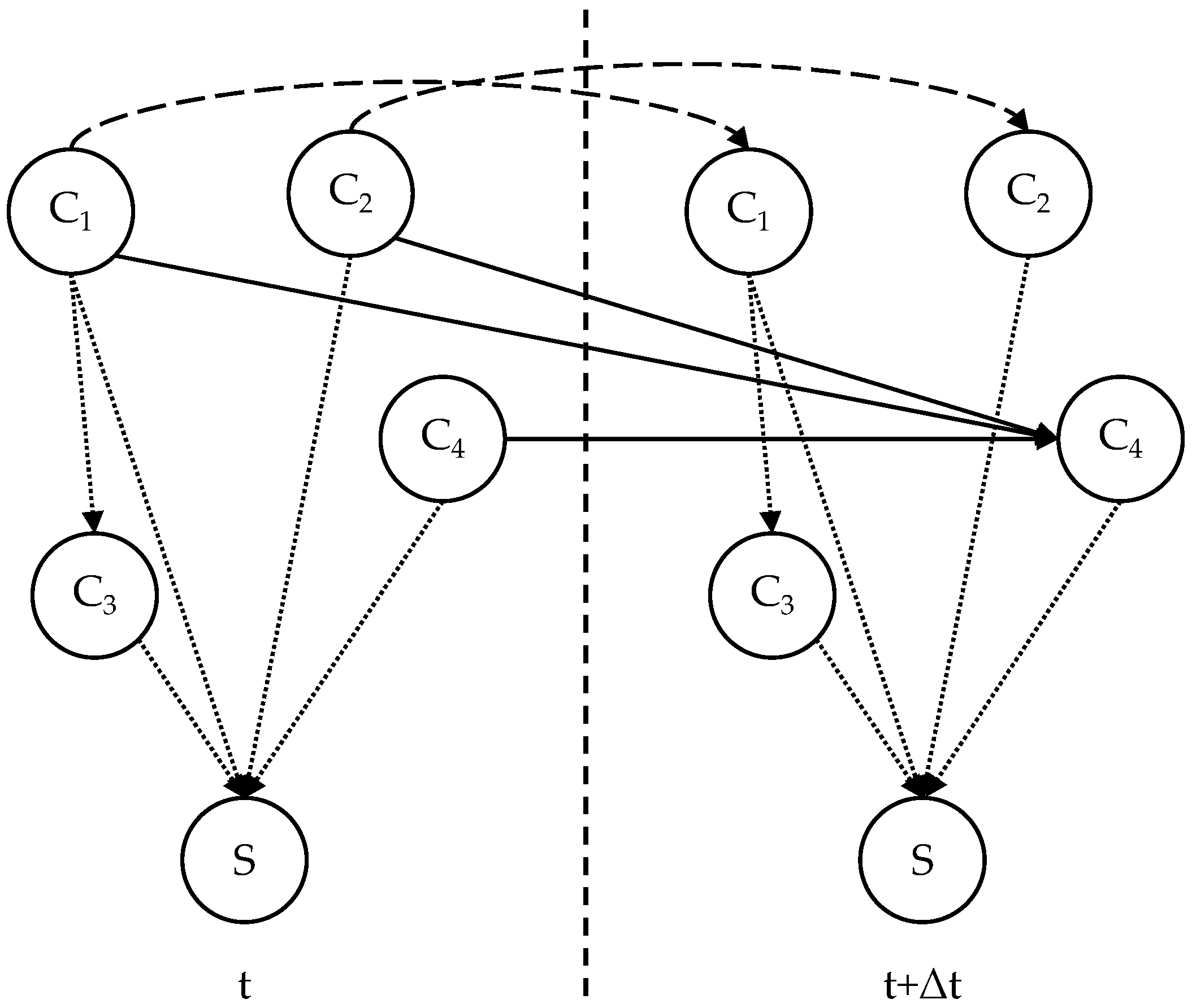
Without loss of generality, a PHM-DBN model is designed as shown in Figure 1 to illustrate the aforementioned properties. The system includes four components, represented by nodes C₁ to C₄, and a system-level node S. The failure type and state space of each node are defined in

Table 2. Assumptions of each node.

Node	Node Type	State Space
C1	Discrete	2 states
C2	Degradation	Continuous stochastic process
C3	Degradation	K discrete states
C4	Discrete	2 states

.

The DBN contains three types of directed edges, representing three different meanings, as detailed below.

• Static failure interaction between components

Dotted edges between nodes within the same time slice represent static failure dependencies between components, which are quantified using conditional probability tables (CPTs). For example, the directed edge C₁ → C₃ is defined by the CPT in

Table 3. CPT of C₁ → C₃.

State of C1	State of C3
	0	1	…	K − 1
0	a00	a01	…	a0K−1
1	a10	a11	…	a1K−1

, where $a_{ij}\ge 0$ and $\sum _{j=0}^{K-1}{a}_{ij}=1$, i = 0, 1.

As the failure of any component leads to system malfunction, the CPT of {C₁, C₂, C₃, C₄} → S is defined as follows:

$$S=\left\{\begin{array}{cc}0& \mathrm{N}\mathrm{o}\mathrm{ }\mathrm{c}\mathrm{o}\mathrm{m}\mathrm{p}\mathrm{o}\mathrm{n}\mathrm{e}\mathrm{n}\mathrm{t}\mathrm{s}\mathrm{ }\mathrm{f}\mathrm{a}\mathrm{i}\mathrm{l}\mathrm{i}\mathrm{n}\mathrm{g}\\ 1& \mathrm{o}\mathrm{t}\mathrm{h}\mathrm{e}\mathrm{r}\mathrm{w}\mathrm{i}\mathrm{s}\mathrm{e}\end{array}\right.,$$

(3)

2.

Dynamic evolution of single component failure process

Dashed edges connecting the same component across consecutive time slices represent the temporal evolution of its failure process. The time interval Δt is assumed sufficiently small such that no state transition occurs within it. For the discrete component C₁, the CPT of C₁(t) → C₁(t + Δt) is given in

Table 4. CPT of $C_1(t)\to C_1(t + \mathsf{\Delta }t)$.

$\mathbf{State} \mathbf{of} {\mathit{C}}_1(\mathit{t})$	$\mathbf{State} \mathbf{of} {\mathit{C}}_1(\mathit{t} + \mathit{\Delta }\mathit{t})$
	0	1
0	${\displaystyle \frac{R_1(t + \mathsf{\Delta }\mathrm{t})}{R_1(t)}}$	$1-{\displaystyle \frac{R_1(t + \Delta t)}{R_1(t)}}$
1	0	1

, where R₁(·) is the reliability function of C₁.

For the degrading component C₂, its continuous stochastic degradation process is discretized into a multi-state Markov process [22], and then the Markov transition probability can be represented using CPT. The steps are as follows: Assume that the state space of degradation component i is divided into $\{\mathrm{0,1},\dots ,M_i\}$, with a failure threshold is set as D_i. Let $d_i={\displaystyle \frac{D_i}{M_i}}$ denote the interval width for discretizing the degradation process. For $\forall m_i\in \{\mathrm{0,1},\dots ,M_i-1\}$, if $Y_i(t)\in [m_i{d}_i,(m_i+1)d_i)$, the component is considered to be in state ${\mathrm{m}}_{\mathrm{i}}$, whereas if $Y_i(t)\in [D_i,+\infty )$, the component is considered to be in state $M_i$, i.e., the failure state, which is the absorbing state of the Markov process. After discretization, the CPT of C₂(t) → C₂(t + Δt) is given in

Table 5. CPT of C₂(t) → C₂(t + Δt).

$\mathbf{State} \mathbf{of} {\mathit{C}}_2(\mathit{t})$	$\mathbf{State} \mathbf{of} {\mathit{C}}_2(\mathit{t} + \mathsf{\Delta }\mathit{t})$
	0	1	2	…	${\mathit{M}}_2$
0	$P_{(\mathrm{0,0})}^2$	$P_{(\mathrm{0,1})}^2$	$P_{(\mathrm{0,2})}^2$	…	$P_{(0,M_2)}^2$
1	$P_{(\mathrm{1,0})}^2$	$P_{(\mathrm{1,1})}^2$	$P_{(\mathrm{1,2})}^2$	…	$P_{(1,M_2)}^2$
2	$P_{(\mathrm{2,0})}^2$	$P_{(\mathrm{2,1})}^2$	$P_{(\mathrm{2,2})}^2$	…	$P_{(2,M_2)}^2$
…	…	…	…	…	…
$M_2$	0	0	0	…	1

, where

$$P_{(j,k)}^i=\left\{\begin{array}{cc}{\int }_{j{d}_i}^{(j+1)d_i}{f}_{Y_j}\left(y-(j+0.5)d_i\right)\mathrm{d}y,& \mathrm{f}\mathrm{o}\mathrm{r}\mathrm{ }j=0,\mathrm{ }1,\mathrm{ }\dots ,\mathrm{ }{M}_i-1;\mathrm{ }k=0,\mathrm{ }1,\mathrm{ }\dots ,M_i-1\\ {\int }_{D_i}^{+\mathrm{\infty }}{f}_{Y_j}\left(y-(j+0.5)d_i\right)\mathrm{d}y,& \mathrm{f}\mathrm{o}\mathrm{r}\mathrm{ }j=0,\mathrm{ }1,\mathrm{ }\dots ,\mathrm{ }{M}_i-1;\mathrm{ }k=M_i\end{array}\right.,$$

(4)

and $f_{Y_j}(\cdot )$ is defined in Equation (2).

3.

Dynamic failure interactions between components

Solid edges in Figure 1 connect nodes C₁, C₂, and C₄ across time slices, representing dynamic and mixed failure interactions. These are modeled using a PHM:

$$h_4\left(t,\mathit{Z}(t)\right)=h_{40}\left(t\right)\phi (\mathit{\gamma },\mathit{Z}(t)),$$

(5)

where $h_{40}\left(t\right)$ is the baseline hazard rate of C₄, which depends on the failure distribution of C₄. $\phi (\mathit{\gamma },\mathit{Z}(t))$ is the link function capturing the effect of covariates on the failure process of C₄, γ is the coefficient and Z(t) represents the covariates based on the states of C₁ and C₂. Then, the conditional reliability function of C₄ is:

$$R_4(t+\Delta t|t,\mathit{Z}(t))=P\left(\zeta \ge t+\Delta t|\zeta \ge t, \mathit{Z}(t)\right)=\mathbb{E}\left[\exp \left(-{\int }_t^{t+\Delta t}{h}_{40}(s)\phi (\mathit{\gamma },\mathit{Z}(s)) \mathrm{d}s\right)|\mathit{Z}(t)\right],$$

(6)

As the number of covariates and state increases, obtaining an analytical solution for Equation (6) becomes challenging. Therefore, an approximation method is adopted [23] with the following assumptions:

(1)

The component state deteriorates continuously over time; that is, the baseline hazard function is nondecreasing.

(2)

The covariate process is nondecreasing, meaning Z(t + Δt) ≥ Z(t) for any Δt > 0. This is reasonable in most practical scenarios, as covariates in this context correspond to the states of other components. This implies that both the link function and the hazard rate function are also nondecreasing.

The above assumptions align with engineering practice, leading to:

$${\int }_t^{t+\Delta t}{h}_{40}(s)\phi (\mathit{\gamma },\mathit{Z}(s)) \mathrm{d}s\ge {\int }_t^{t+\Delta t}{h}_{40}(s)\phi (\mathit{\gamma },\mathit{Z}(t)) \mathrm{d}s=\phi (\mathit{\gamma },\mathit{Z}(t)){\int }_t^{t+\Delta t}{h}_{40}(s) \mathrm{d}s,$$

(7)

$${\int }_t^{t+\Delta t}{h}_{40}(s)\phi (\mathit{\gamma },\mathit{Z}(s)) \mathrm{d}s\le {\int }_t^{t+\Delta t}{h}_{40}(s)\phi (\mathit{\gamma },\mathit{Z}(t+\Delta t)) \mathrm{d}s=\phi (\mathit{\gamma },\mathit{Z}(t+\Delta t)){\int }_t^{t+\Delta t}{h}_{40}(s) \mathrm{d}s,$$

(8)

$$\underset{\Delta \mathit{t}\to 0}{\lim }\phi (\mathit{\gamma },\mathit{Z}(t+\Delta t))-\phi (\mathit{\gamma },\mathit{Z}(t))=0.$$

(9)

Given the assumption that no state transitions occur within Δt when $\Delta t$ is sufficiently small, Equations (7) and (8) are very close and build the upper and lower bound of Equation (6). Thus, Equation (6) can be approximated to:

$$R_4(t+\Delta t|t,\mathit{Z}(t))=\mathbb{E}\left[\exp \left(-{\int }_t^{t+\Delta t}{h}_{40}\left(s\right)\phi (\mathit{\gamma },\mathit{Z}(s)) \mathrm{d}s\right)|\mathit{Z}(t)\right]\approx \exp \left(-\phi (\mathit{\gamma },\mathit{Z}(t)) {\int }_t^{t+\Delta t}{h}_{40}\left(s\right)\mathrm{d}s\right).$$

(10)

Equation (10) allows the PHM to be converted into CPT. The CPT for the edge {C₁(t), C₂(t), C₄(t)} → C₄(t + Δt) is provided in

Table 6. CPT of {C₁(t), C₂(t), C₄(t)} → C₄(t + Δt).

$\mathbf{State} \mathbf{of} {\mathit{C}}_1(\mathit{t}),{\mathit{C}}_2(\mathit{t}),{\mathit{C}}_4(\mathit{t})$	$\mathbf{State} \mathbf{of} {\mathit{C}}_4(\mathit{t} + \mathit{\Delta }\mathit{t})$
	0	1
$C_4(t)=0,\mathit{Z}(t)=C_1(t),C_2(t)$	$R_4(t+\mathsf{\Delta }t|t,\mathit{Z}(t))$	$1-R_4(t+\mathsf{\Delta }t|t,\mathit{Z}(t))$
$C_4(t)=1,\mathit{Z}(t)=C_1(t),C_2(t)$	0	1

.

2.3. Parameter Learning of the PHM-DBN Model

Since all the above failure models and failure interactions have been transformed into the DBN representation, the parameter learning of the PHM-DBN model essentially involves parameter learning for the DBN model. This includes two aspects: (1) Parameter learning for the component nodes’ failure models; and (2) Parameter learning for the directed edges representing failure interactions, which can be performed independently.

The parameter learning method for each component node’s failure model depends on the component’s failure type and pre-defined failure model.

Table 7. Parameter learning of component nodes.

Component Node	Failure Type	Failure Model	Data Source	Parameter Learning Method
C1, C4	Discrete	Failure time distribution function	Component failure time data	Maximum Likelihood estimation (MLE), Bayesian estimation
C2	Degradation	Continuous stochastic process	Component condition monitoring data	MLE, Bayesian estimation
C3	Degradation	Multi-state Markov process	Component condition monitoring data	Frequency count method, MLE, Expectation maximization, Bayesian estimation

summarizes the required data sources and applicable parameter learning methods. Among these methods, techniques such as Maximum Likelihood Estimation (MLE) and Bayesian estimation are standardized processes in the reliability engineering field, and detailed implementations can be found in references [24,25].

As described in Section 2.2, the three types of directed edges in the model are all converted into CPT. The first type of CPT represents the conditional probabilities of failure states between components. The second type denotes the state transition probabilities of the same node over time. The third type directly transforms the covariate-hazard rate relationship estimated by the PHM into a DBN-compatible CPT, which is the centerpiece of the PHM-DBN coupling and achieves mathematical compatibility between the two models. Thus, the CPT can be derived directly from the PHM parameter learning results without additional parameter estimation.

Table 8. Parameter learning of directed edges.

Directed Edge Type	CPT Representation	Data Source	Parameter Learning Method
Type 1	Conditional probability	State or failure data of parent nodes and child nodes (require strictly synchronous collection)	MLE, Bayesian estimation, expert elicitation
Type 2	State transition probability	Component time-series state data	MLE, Bayesian estimation, or derived from component failure model
Type 3	PHM	Component failure data along with covariates’ time-series state data (require strictly synchronous collection)	MLE, Bayesian estimation

lists the required data sources and available parameter learning methods for these CPTs, which follow standardized procedures in both DBN and PHM research. Since this study focuses on optimal maintenance decision-making, the detailed steps for CPT and PHM parameter learning are not elaborated further and can be referred to in [26,27,28,29,30,31].

3. MDP-Based Maintenance Decision Formulation

The DBN model in Section 2 characterizes the state space and probability transition of multi-component systems. By further incorporating elements such as maintenance actions and associated costs, a five-tuple Markov Decision Process model can be constructed, thereby enabling the optimization of maintenance policies [17].

3.1. State and Action Spaces

The overall state space of system is denoted as S = {C₁, C₂, …, C_N}, where C_i (i = 1, 2, …, N) represents the state of component i, corresponding to node states in the DBN. If component i has a discrete failure mode, its state space is C_i ∈ {0, 1}, whereas if component i is a degradation component, the discretized state space is C_i ∈ {0, 1, …, M_i}.

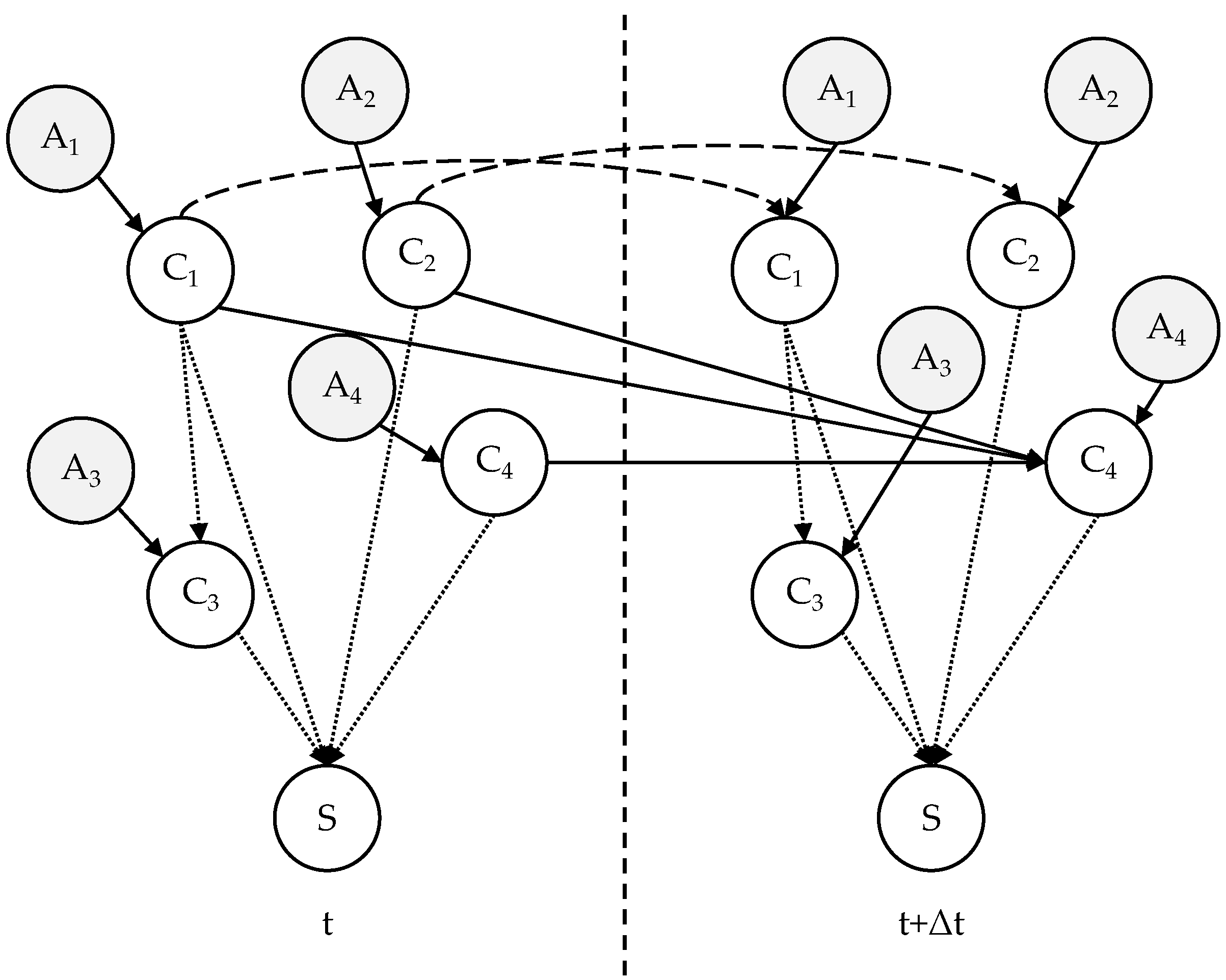
Action nodes can be introduced into DBN to define the state-action transition probabilities [23]. As shown in Figure 2, each component node is associated with an action node A_i, connected via a directed edge. The collective action space of the system is A = {A₁, A₂, …, A_N}. A single action A_i is performed on component i with A_i ∈ {0, CM_i, PM_i}, defined as follows:

A_i = 0: Do nothing. The state of component i remains unchanged.

A_i = CM_i: Corrective maintenance. Applied when a discrete component has failed or a degrading component has reached state M_i. This action resets the age of a discrete component or the degradation state of a degrading component to 0.

A_i = PM_i: Preventive maintenance. This action is only available for degrading components. It reduces the degradation state proportionally; i.e., ${Y_i}^{\prime }(t)=\alpha \cdot Y_i(t)$, where α ∈ (0,1) is the reduction factor.

3.2. State-Action Transition Probabilities

When the states of all action nodes within the same time slice are specified, the state-action transition probabilities of component nodes can be deterministically defined using CPT. It is assumed that maintenance actions take effect immediately; that is, the node state at $t+\mathsf{\Delta }t$ is determined based on the post-maintenance state at time t. Taking nodes C₁ and C₂ as examples, the state-action transition probabilities are defined in

Table 9. State-action transition probabilities of C₁, given ${ A}_1(t)={CM}_1$.

$\mathbf{State} \mathbf{of} {\mathit{C}}_1(\mathit{t})$	$\mathbf{State} \mathbf{of} {\mathit{C}}_1(\mathit{t} + \mathsf{\Delta }\mathit{t})$
	0	1
$C_1(t)=0$ or $C_1(t)=1$	${\displaystyle \frac{R(\mathsf{\Delta }t)}{R(0)}}$	$1-{\displaystyle \frac{R(\mathsf{\Delta }t)}{R(0)}}$

,

Table 10. State-action transition probabilities of C₂, given ${ A}_2(t)={CM}_2$.

$\mathbf{State} \mathbf{of} {\mathit{C}}_2(\mathit{t})$	$\mathbf{State} \mathbf{of} {\mathit{C}}_2(\mathit{t} + \mathsf{\Delta }\mathit{t})$
	0	1	2	…	${\mathit{M}}_2$
$C_2(t)=\mathrm{0,1},2,\dots ,M_2$	$P_{(\mathrm{0,0})}^2$	$P_{(\mathrm{0,1})}^2$	$P_{(\mathrm{0,2})}^2$	…	$P_{(0,M_2)}^2$

and

Table 11. State-action transition probabilities of C₂, given ${ A}_2(t)={PM}_2$.

$\mathbf{State} \mathbf{of} {\mathit{C}}_2(\mathit{t})$	$\mathbf{State} \mathbf{of} {\mathit{C}}_2(\mathit{t} + \mathsf{\Delta }\mathit{t})$
	0	1	2	…	${\mathit{M}}_2$
0	$P_{(\mathrm{0,0})}^2$	$P_{(\mathrm{0,1})}^2$	$P_{(\mathrm{0,2})}^2$	…	$P_{(0,M_2)}^2$
1	$P_{({\alpha }_1,0)}^2$	$P_{({\alpha }_1,1)}^2$	$P_{({\alpha }_1,2)}^2$	…	$P_{({\alpha }_1,M_2)}^2$
2	$P_{({\alpha }_2,0)}^2$	$P_{({\alpha }_2,1)}^2$	$P_{({\alpha }_2,2)}^2$	…	$P_{({\alpha }_2,M_2)}^2$
…	…	…	…	…	…
$M_2$	$P_{({\alpha }_{M_2},0)}^2$	$P_{({\alpha }_{M_2},1)}^2$	$P_{({\alpha }_{M_2},2)}^2$	…	$P_{({\alpha }_{M_2},M_2)}^2$

.

Where ${\alpha }_m(m=\mathrm{1,2},\dots ,M_2)$ quantifies the effect of preventive maintenance on the component state under imperfect maintenance, which is determined according to the interval in which ${Y_2}^{\prime }(t)$ falls by Equation (4).

Similarly, the state–action transition probabilities of nodes C₃ and C₄ can be derived via DBN inference, given the states of their parent nodes (including action nodes and other component nodes).

3.3. Reward Setting

The cost associated with maintenance actions at each decision epoch consists of the following:

Corrective Maintenance (CM) Cost: Includes unplanned downtime cost $c_d$ and maintenance cost $c_i^c$ for component undergoing CM. The total cost is $c_{\mathrm{d}}+\sum _{i\in \mathit{C}\mathit{M}}{c}_i^c$, where CM is the set of components receiving CM.

Preventive Maintenance (PM) Cost: Includes a fixed setup cost $c_s$ and maintenance cost $c_j^p$ for component undergoing PM. The total cost is $c_s+\sum _{j\in \mathit{P}\mathit{M}}{c}_j^p$, where PM is the set of components receiving PM.

Then the immediate cost $R(s,a)$ at each decision epoch is defined as:

$$R(\mathit{S},\mathit{A})=\left\{\begin{array}{cc}0& if \mathit{C}\mathit{M}=\mathit{\varnothing }\mathit{ }\&\mathit{ }\mathit{P}\mathit{M}=\mathit{\varnothing }\\ -\left[c_d+c_s+\sum _{i\in \mathit{C}\mathit{M}}{c}_{i,C}+\sum _{j\in \mathit{P}\mathit{M}}{c}_{j,P}\right]& \mathrm{e}\mathrm{l}\mathrm{s}\mathrm{e}\end{array}\right..$$

(11)

3.4. MDP Maintenance Optimization

The transition probabilities of the proposed MDP model are non-stationary. Therefore, the maintenance policies are optimized using a finite horizon discrete time MDP framework. Given a planning horizon T and time step Δt, the number of decision epochs H is $H=\lfloor T/∆t\rfloor +1$. The selection of planning horizon is guided by two core engineering principles: one aligns with component reliability characteristics, meaning the time horizon must cover at least one complete “degradation-failure-maintenance” cycle of critical components to ensure optimal decisions account for long-term reliability. The other reflects industrial maintenance practices, planning horizon is typically developed for fixed short-to-medium-term cycles to balance decision flexibility and resource planning, enabling adaptation to real-time state changes while avoiding myopic decision-making.

The objective is to maximize the total expected reward over the horizon. This is achieved using backward induction in dynamic programming. The process starts from the final epoch H and proceeds backward to the first epoch. The Bellman equation for the state-value function at each decision epoch h = {1, 2, …, H} is constructed as follows:

$$V_h(\mathit{S})=\underset{a\in A}{\max }[R(\mathit{S},\mathit{A})+\gamma {\sum }_{s^{\prime }\in S}{P}_h({\mathit{S}}^{\prime }|\mathit{S},\mathit{A})V_{h+1}({\mathit{S}}^{\prime })],$$

(12)

where $V_{\mathrm{H}}(s)=0$ for all terminal states. The discount factor $\gamma$ (0 ≤ $\gamma$ ≤ 1) is typically used to balance the weight of immediate and future rewards, $\gamma$ < 1 avoids infinite total reward and ensures the convergence of value iteration. However, for finite-horizon MDP, the decision-making process is bounded by a clear time endpoint, and future rewards within the horizon are equally relevant to the overall optimization objective, so $\gamma$ can be set to 1 in this study. The optimal policy at each state s and epoch h is

$${\pi }_h(\mathit{S})=\underset{a\in A}{\mathrm{arg max}}[R(\mathit{S},\mathit{A})+\gamma {\sum }_{s^{\prime }\in S}{P}_h({\mathit{S}}^{\prime }|\mathit{S},\mathit{A})V_{h+1}({\mathit{S}}^{\prime })].$$

(13)

At each decision epoch h, $P_h({\mathit{S}}^{\prime }|\mathit{S},\mathit{A})$ is the probability of transitioning to state $s^{\prime }$ given action a at state s.

In traditional MDP formulations for multi-component systems, state space complexity constitutes the primary computational bottleneck. This is because the total number of system states equals the product of the state counts of individual components, which grows exponentially with N, and increases the cost of calculating state transition probabilities. However, the DBN model is designed to decompose the joint state space using conditional independence assumptions, thereby reducing computational complexity [18]. In DBN model, each component’s state depends only on its parent nodes, not all other components. Mathematically, the joint probability of the system state $\mathit{S}(t)=\{C_1(t),C_2(t),\dots ,C_N(t)\}$ can be decomposed as:

$$P(\mathbf{S})={\displaystyle {\prod }_{i=1}^N}P(C_i\mid \mathrm{P}\mathrm{a}\mathrm{r}\mathrm{e}\mathrm{n}\mathrm{t}\mathrm{s}(C_i)),$$

(14)

where $\mathrm{P}\mathrm{a}\mathrm{r}\mathrm{e}\mathrm{n}\mathrm{t}\mathrm{s}(C_i(t))$ are the parent nodes of component i in the DBN. This decomposition reduces the number of parameters needed to describe the joint state.

The transition probability can also be decomposed using the DBN’s time-slice dependencies:

$$P({\mathit{S}}^{\prime }|\mathit{S},\mathit{A})={\displaystyle {\prod }_{i=1}^N}P(C_i(t+\mathsf{\Delta }t)\mid \mathrm{P}\mathrm{a}\mathrm{r}\mathrm{e}\mathrm{n}\mathrm{t}\mathrm{s}(C_i(t)),\mathit{A}),$$

(15)

Each component’s transition is computed independently using its CPT, eliminating the need to enumerate all possible joint state transitions. Leveraging this characteristic, the DBN structure significantly reduces the computational burden associated with state transition probability calculations. A formal complexity comparison between the proposed framework and traditional MDP is provided in

Table 12. Computational complexity comparison.

Metric	Traditional MDP	MDP with DBN Inference
Joint State Parameters	$O(\prod _{i=1}^N{C}_i)$	$O\left(\sum _{i=1}^N\left(C_i\times {\prod }_{\mathrm{p}\mathsf{ϵ}\mathrm{P}\mathrm{a}\mathrm{r}\mathrm{e}\mathrm{n}\mathrm{t}\mathrm{s}(C_i)}{C}_p\right)\right)$
Transition Probability Calculations	$O\left({\left(\prod _{i=1}^N{C}_i\right)}^2\right)$	$O\left({\prod }_{\mathrm{p}\mathsf{ϵ}\mathrm{P}\mathrm{a}\mathrm{r}\mathrm{e}\mathrm{n}\mathrm{t}\mathrm{s}(C_i\left(\mathrm{t}+\mathsf{\Delta }t\right))}{C}_p\right)$

.

4. Numerical Study

Here, we present a numerical case study in which the proposed model is applied to the CBM of multi-component systems. The target system for demonstration remains the DBN illustrated in Figure 1. Thanks to its flexibility, this system can represent various types of industrial assets, such as manufacturing systems, rotating machinery, power systems, and transportation equipment, and can be extended with additional nodes and attributes tailored to specific practical scenarios.

4.1. Model Definition of the Target System

The proposed model for the target system utilizes data encompassing the failure model, the state space of each component node, interdependencies between node failures, the states of action nodes, and relevant costs. The costs include expenses related to unplanned downtime, planned downtime, and performing CM or PM actions, as shown in

Table 13. Definition of component nodes.

Component Node	Failure Type	Model Parameters	State Space
C1	Exponential distribution	$R(t)=e^{-\lambda t}$, $\lambda =0.02$	{0, 1}
C2	Gamma process	$f_Y\left(y\right)=Ga(y|\nu ,u)={\displaystyle \frac{u^v{y}^{\nu -1}{e}^{-uy}}{\mathsf{\Gamma }(\nu )}},y\ge 0$ $\nu =0.04,u=6,D=7$	{0, 1, 2, …, 7}
C3	Multistate Markov process	$P\left(C_3(t+∆t)|C_3(t)\right)=\left[\begin{array}{ccc}0.7& 0.2& 0.1\\ 0.1& 0.6& 0.3\\ 0& 0& 1\end{array}\right]$	{0, 1, 2}
C4	Weibull distribution	$R(t)=e^{-{\left({\displaystyle \frac{t}{\eta }}\right)}^{\beta -1}},\eta =200,\beta =1.5$	{0, 1}

,

Table 14. Failure interactions between relevant nodes.

Failure Interaction	Definition
C1 → C3	$P\left(C_3(t)|C_1(t)\right)=\left[\begin{array}{ccc}0.8& 0.1& 0.1\\ 0.1& 0.5& 0.4\end{array}\right]$
{C1, C2} → C4	$h_4\left(t,C_1(t),C_2(t)\right)={\displaystyle \frac{\beta }{\eta }}{\left({\displaystyle \frac{t}{\eta }}\right)}^{\beta -1}\ast \mathrm{e}\mathrm{x}\mathrm{p}({\gamma }_1{C}_1(t)+{\gamma }_2{C}_2(t))$ $\eta =200,\beta =1.5,{\gamma }_1=0.1,{\gamma }_2=0.4$

and

Table 15. Definition of action nodes and costs.

Action Node	Action Space	Costs
A1	{0, CM1}	$c_1^c=500$, $c_2^c=750$, $c_3^c=500$, $c_4^c=800$, $c_2^P=100$, $c_3^P=200$, $c_d=5000$, $c_s=350$
A2	{0, CM2, PM2}
A3	{0, CM3, PM3}
A4	{0, CM4}

.

The methodology proceeds in two main steps. First, the DBN model of the system is established, and the states of its nodes are inferred using the BNT toolbox in MATLAB R2020a [32]. Second, the optimal maintenance policies are obtained by solving the MDP model through the backward induction algorithm.

4.2. Results Discussion and Comparison

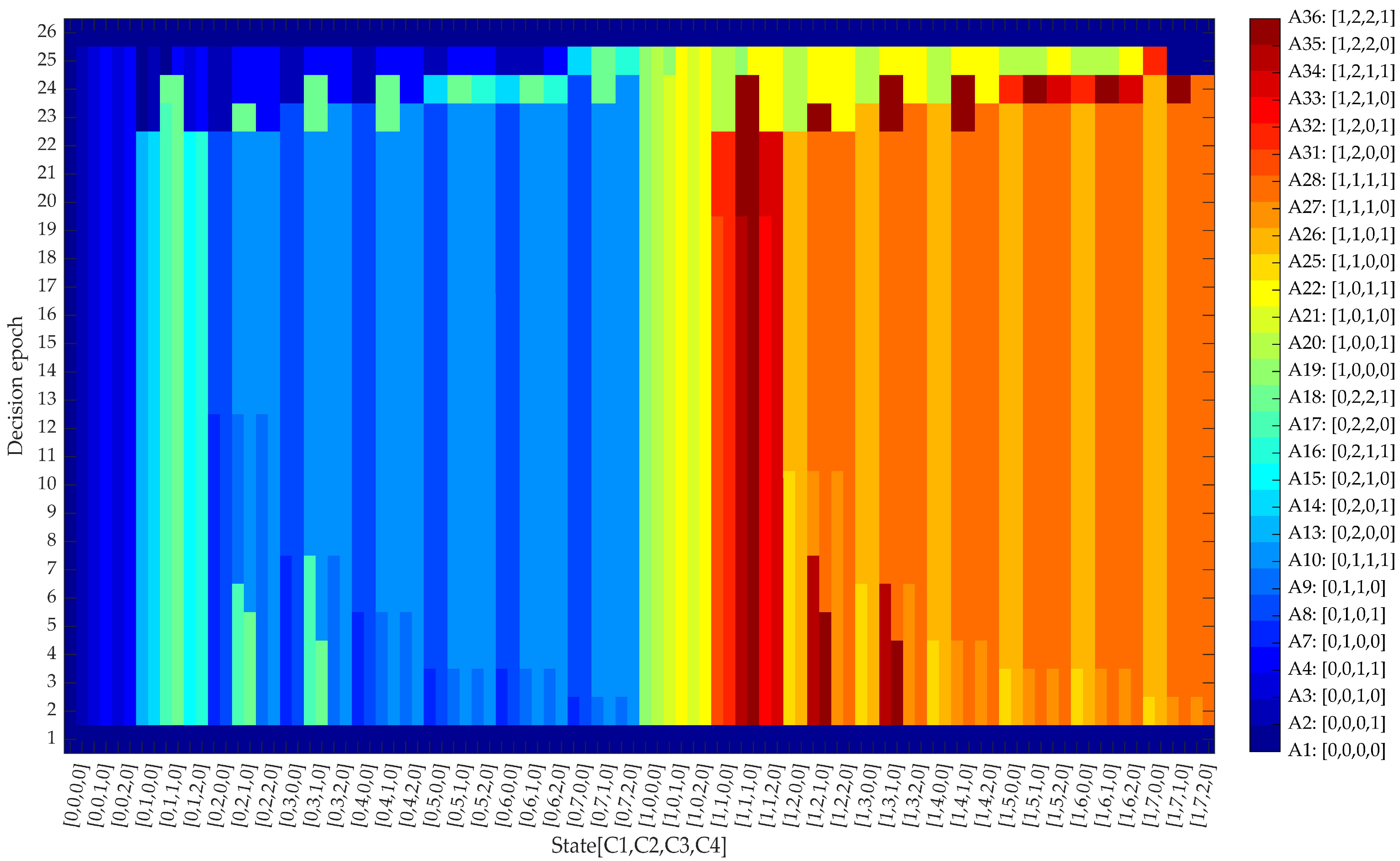
The maintenance planning horizon is set to T = 500 with a discrete time step of Δt = 20. For different initial system states, the optimal maintenance actions are derived directly from the MDP solution and visualized as a heatmap in Figure 3. The key insights from the results are summarized as follows:

• As the initial degradation state of component C₂ increases, the optimal strategy shifts progressively from PM₂ to CM₂. This indicates that postponing corrective maintenance too long becomes economically unfavorable for an aged component.
• When C₂ begins in a degraded state (C₂ ≥ 2), the maintenance strategy over time includes CM₄ for component C₄,even before C₄ has failed. This is due to the failure dependence between C₂ and C₄, which elevates the failure risk of C₄. Thus, performing joint maintenance yields greater long-term benefits than maintaining a single component.
• When multiple components require maintenance simultaneously, joint corrective or preventive actions are generally more cost-effective than maintaining components individually. This advantage stems from the sharing of downtime and setup costs. Despite the additional maintenance expenses incurred, the overall long-term value is improved.
• As the system ages, the maintenance strategy increasingly prioritizes short-term gains. Consequently, in the later stages of the planning horizon, actions with minimal immediate cost tend to be selected—including, in some cases, the option of performing no maintenance.

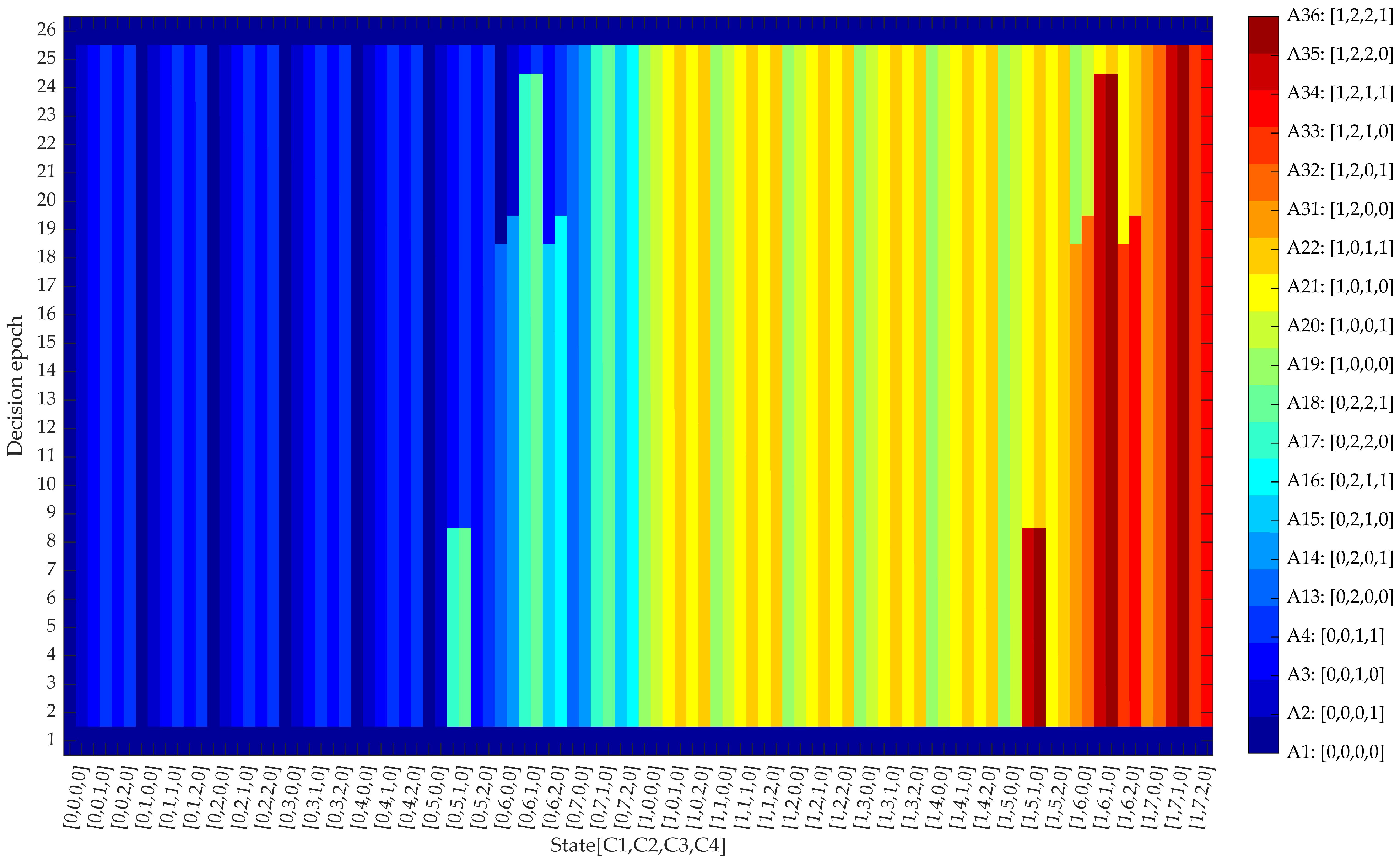
A comparative study between the independence assumption and our proposed model was conducted. Under the independence assumption, failure interactions between components are ignored, and the resulting optimal maintenance strategy derived from the MDP solution is shown in Figure 4. In contrast to the strategy in Figure 3, the independence-based approach tends to focus more on the long-term benefit of individual components, exhibits greater conservatism in joint maintenance, and only triggers maintenance when the degradation state becomes more severe. For example, C₂ and C₃ are initiated only when C₂ > 5 and C₃ = 1. Moreover, due to the neglect of failure impact, the maintenance strategy does not consider adding CM action for C₄.

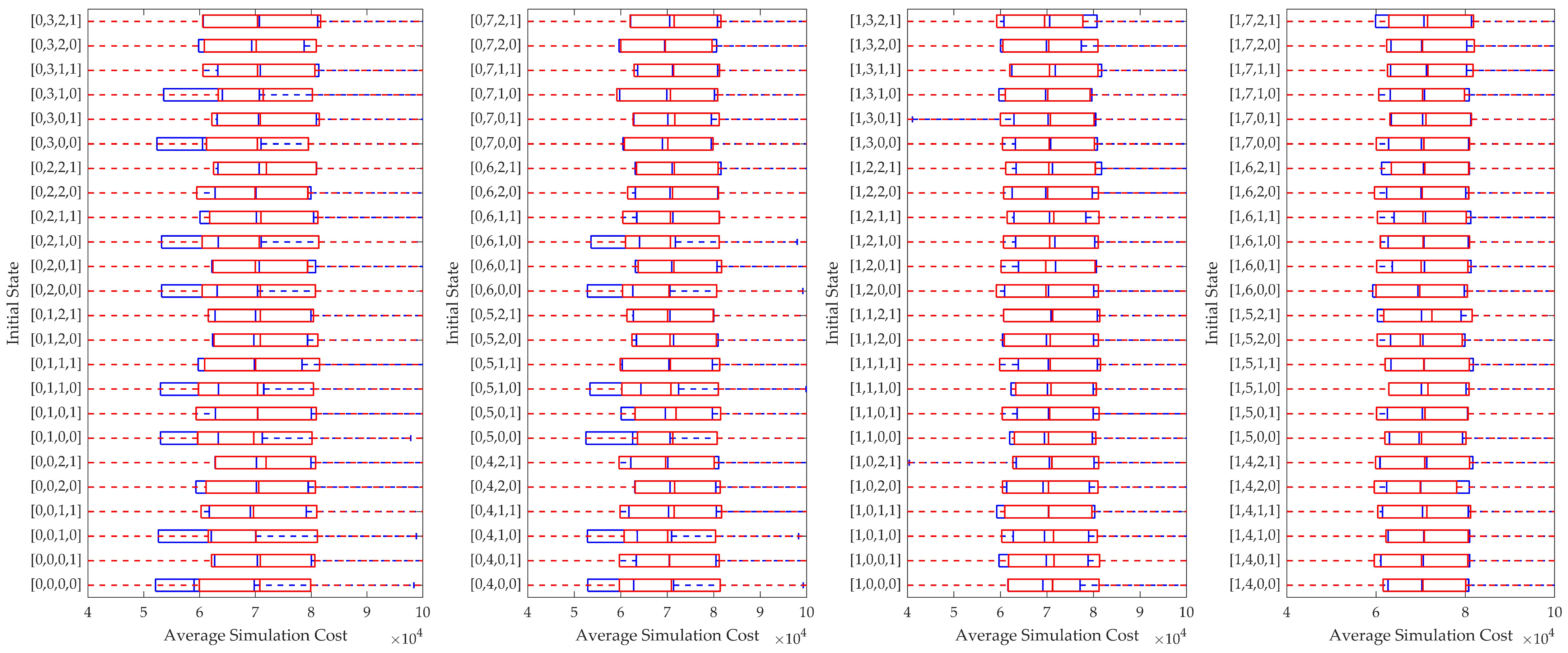
Additionally, a comparative analysis of system operating costs under the independence assumption and the proposed dependency-aware assumption was conducted. The system operation was simulated 500 times for each of 96 different initial states, and the average operating costs under the two assumptions were calculated, as shown in Figure 5, where the blue and red boxplots represent the average operating costs of the proposed model and the independence assumption, respectively. The results indicate that in 59 out of the 96 initial states, the proposed method reduces the average operating cost by 10%.

To comprehensively verify the effectiveness and practical superiority of the proposed framework, we conducted comparative experiments against two maintenance policies, which cover the most widely adopted maintenance paradigms in engineering practice, ensuring the comparison reflects real-world decision scenarios. All experiments were performed via 500 independent Monte Carlo simulations, with results reported as total expected cost and system availability. The baseline policies selected for comparison are defined as follows:

(1)

Corrective Maintenance (CM-only): Maintenance actions are only initiated after a component fails, with no preventive measures.

(2)

Threshold Based Proactive Maintenance via DBN [17] (ThPM-DBN): A predictive maintenance strategy that considers the system reliability; if system reliability is less than a given threshold, a proactive maintenance is scheduled.

The comparative performance of the proposed framework and baseline policies is summarized in Table 15. Compared to the best in policy

Table 16. Comparative Results Against Baseline Policies.

Maintenance Policy	Total Expected Cost	System Availability
CM-only	70,062 ± 12,608	0.7707 ± 0.0066
ThPM-DBN (threshold = 0.99)	66,567 ± 13,955	0.9611 ± 0.0055
ThPM-DBN (threshold = 0.95)	68,906 ± 13,323	0.9168 ± 0.0042
ThPM-DBN (threshold = 0.9)	70,201 ± 14,411	0.8764 ± 0.0051
Our model	61,610 ± 13,908	0.9788 ± 0.0043

, our framework still delivers at least 8.1% reduction in total expected cost, with a modest 1.8% improvement in system availability. It demonstrates that the proposed PHM-DBN-MDP framework outperforms traditional maintenance policies in both cost reduction and availability improvement. The core advantage lies in its ability to integrate mixed failure type modeling, dependency quantification, and state-aware optimization. These results confirm the framework’s practical effectiveness and competitiveness for industrial condition-based maintenance decision-making.

4.3. Sensitivity Analysis

Component-related costs including PM cost, CM cost, and system downtime cost are critical inputs for the MDP reward function. In industrial practice, these costs are often estimated with uncertainties. To evaluate the framework’s robustness to such variations, we tested three cost fluctuation levels: ±20%, ±40% relative to the baseline cost parameters in

Table 17. Sensitivity Results to Component Cost Fluctuations.

Maintenance Policy	Total Expected Cost	System Availability
40%	84,749 ± 18,234	0.9791 ± 0.0046
20%	73,462 ± 16,491	0.9788 ± 0.0051
0% (baseline)	61,610 ± 13,908	0.9788 ± 0.0043
−20%	50,240 ± 9986	0.9783 ± 0.0044
−40%	35,822 ± 7161	0.9794 ± 0.0042

. For each level, all component costs were adjusted simultaneously to simulate systemic cost variations, and the framework’s performance was compared to the baseline. Table 16 presents the sensitivity results to component cost fluctuations.

It can be seen that the total expected cost changes proportionally with cost fluctuations, confirming that the MDP reward function correctly incorporates cost inputs without bias. Meanwhile the system availability remains nearly constant across all cost fluctuation levels, which means the framework’s ability to ensure system reliability is not compromised by cost estimation uncertainties. The results indicate that the framework’s performance is linearly responsive to component cost fluctuations but maintains stable decision logic and high robustness.

5. Conclusions

This study proposes a maintenance decision framework for multi-component systems. addressing the core challenge of modeling mixed failure types (discrete/degradation) and complex failure dependencies (static/dynamic/mixed) that limit the applicability of existing methods. By innovatively integrating the proportional hazards model into a dynamic Bayesian network and coupling the hybrid model with a finite-horizon Markov Decision Process, the framework achieves characterization of failure evolution, dependency quantification, and maintenance optimization. A systematic numerical study was conducted to validate the framework’s effectiveness, with comprehensive comparisons against baseline policies. Compared to the best result of CM and DBN-based PM policy, the proposed framework reduces total expected cost by 8.1%, while improving system availability by 1.8%, confirming the framework’s superiority in balancing cost efficiency and system reliability.

The primary innovation of this work lies in the dynamic, mathematically compatible coupling mechanism between DBN and PHM. This coupling enables three key breakthroughs: (1) comprehensive coverage of all three typical failure dependencies in multi-component systems, resolving the limitation of traditional DBNs in modeling mixed-type interactions and PHMs in handling multi-component scalability; (2) direct transformation of PHM’s covariate-hazard rate relationship into DBN’s CPT via approximation, achieving seamless integration with DBN’s probabilistic inference; and (3) a unified MDP-DBN framework that embeds maintenance actions and cost structures, enabling end-to-end condition-based decision-making.

Despite its effectiveness, the framework has three notable limitations that guide future refinement. (1) Fixed operating environment assumption: The study assumes a static operating environment, failing to account for the dynamic nature of real-world conditions (e.g., variable loads, environmental fluctuations) that can dynamically alter component degradation states and failure risks. (2) Lack of inspection integration: The current model only considers CM and PM actions, without incorporating inspection processes. This limits the ability to obtain accurate real-time component state information, hindering refined maintenance decision-making. (3) Scalability constraints for large-scale systems: As the number of components and maintenance action types increases, the state space of the MDP expands significantly. Although the conditional independence of DBN mitigates partial computational burden, the framework still faces challenges in efficiently handling large-scale systems with extensive components and complex interactions.

To enhance practical applicability and address the above limitations, future work will focus on three verifiable objectives aligned with industrial needs: (1) Extend the model to incorporate time-varying operating environments and analyze their impacts on component degradation and failure dependencies, developing adaptive maintenance strategies that respond to real-time environmental variations. (2) Introduce inspection nodes and related costs into the DBN-PHM-MDP framework, optimizing inspection frequency and timing based on component degradation states. This will improve the accuracy of state estimation and enable more targeted, cost-effective maintenance decisions. (3) Explore advanced algorithms such as factored MDP [33], approximate dynamic programming, or deep reinforcement learning to address the state space explosion problem. This will enhance the framework’s scalability and computational efficiency for large-scale multi-component systems.

References

1. Olde Keizer, M.C.A.; Flapper, S.D.P.; Teunter, R.H. Condition-Based Maintenance Policies for Systems with Multiple Dependent Components: A Review. Eur. J. Oper. Res. 2017, 261, 405–420. [Google Scholar] [CrossRef]
2. Zhao, J.; Gao, C.; Tang, T. A Review of Sustainable Maintenance Strategies for Single Component and Multicomponent Equipment. Sustainability 2022, 14, 2992. [Google Scholar] [CrossRef]
3. Li, R.; Cai, B.; Zhao, Y.; Liu, Y.; Zhang, Y.; Kong, X.; Liu, Y. Condition-Based Maintenance Method for Multi-Component Systems under Discrete-State Condition: Subsea Production System as a Case. Ocean Eng. 2024, 306, 118166. [Google Scholar] [CrossRef]
4. Duan, C.; Deng, T.; Song, L.; Wang, M.; Sheng, B. An Adaptive Reliability-Based Maintenance Policy for Mechanical Systems under Variable Environments. Reliab. Eng. Syst. Safe 2023, 238, 109396. [Google Scholar] [CrossRef]
5. Meango, T.J.-M.; Ouali, M.-S. Failure Interaction Models for Multicomponent Systems: A Comparative Study. SN Appl. Sci. 2019, 1, 66. [Google Scholar] [CrossRef]
6. Xu, J.; Liang, Z.; Li, Y.-F.; Wang, K. Generalized Condition-Based Maintenance Optimization for Multi-Component Systems Considering Stochastic Dependency and Imperfect Maintenance. Reliab. Eng. Syst. Safe 2021, 211, 107592. [Google Scholar] [CrossRef]
7. Li, H.; Zhu, W.; Dieulle, L.; Deloux, E. Condition-Based Maintenance Strategies for Stochastically Dependent Systems Using Nested Lévy Copulas. Reliab. Eng. Syst. Safe 2022, 217, 108038. [Google Scholar] [CrossRef]
8. Xu, M.; Jin, X.; Kamarthi, S.; Noor-E-Alam, M. A Failure-Dependency Modeling and State Discretization Approach for Condition-Based Maintenance Optimization of Multi-Component Systems. J. Manuf. Syst. 2018, 47, 141–152. [Google Scholar] [CrossRef]
9. Zhou, H.; Li, Y. Optimal Replacement in a Proportional Hazards Model with Cumulative and Dependent Risks. Comput. Ind. Eng. 2023, 176, 108930. [Google Scholar] [CrossRef]
10. Hu, J.; Chen, P. Predictive Maintenance of Systems Subject to Hard Failure Based on Proportional Hazards Model. Reliab. Eng. Syst. Safe 2020, 196, 106707. [Google Scholar] [CrossRef]
11. Wang, Q.-A.; Chen, J.; Ni, Y.; Xiao, Y.; Liu, N.; Liu, S.; Feng, W. Application of Bayesian Networks in Reliability Assessment: A Systematic Literature Review. Structures 2025, 71, 108098. [Google Scholar] [CrossRef]
12. Cai, B.; Kong, X.; Liu, Y.; Lin, J.; Yuan, X.; Xu, H.; Ji, R. Application of Bayesian Networks in Reliability Evaluation. IEEE Trans. Ind. Inf. 2019, 15, 2146–2157. [Google Scholar] [CrossRef]
13. Luo, X.; Li, Y.; Bai, X.; Tang, R.; Jin, H. A Novel Approach Based on Fault Tree Analysis and Bayesian Network for Multi-State Reliability Analysis of Complex Equipment Systems. Proc. Inst. Mech. Eng. Part O J. Risk Reliab. 2024, 238, 812–838. [Google Scholar] [CrossRef]
14. Ait Mokhtar, E.H.; Laggoune, R.; Chateauneuf, A. Benefit and Customer Demand Approach for Maintenance Optimization of Complex Systems Using Bayesian Networks. Proc. Inst. Mech. Eng. Part O J. Risk Reliab. 2017, 231, 558–572. [Google Scholar] [CrossRef]
15. Hu, J.; Zhang, L.; Liang, W. Opportunistic Predictive Maintenance for Complex Multi-Component Systems Based on DBN-HAZOP Model. Process Saf. Environ. 2012, 90, 376–388. [Google Scholar] [CrossRef]
16. Cai, B.; Liu, Y.; Fan, Q.; Zhang, Y.; Yu, S.; Liu, Z.; Dong, X. Performance Evaluation of Subsea BOP Control Systems Using Dynamic Bayesian Networks with Imperfect Repair and Preventive Maintenance. Eng. Appl. Artif. Intel. 2013, 26, 2661–2672. [Google Scholar] [CrossRef]
17. Özgür-Ünlüakın, D.; Türkali, B. Evaluation of Proactive Maintenance Policies on a Stochastically Dependent Hidden Multi-Component System Using DBNs. Reliab. Eng. Syst. Safe 2021, 211, 107559. [Google Scholar] [CrossRef]
18. Faddoul, R.; Raphael, W.; Soubra, A.-H.; Chateauneuf, A. Incorporating Bayesian Networks in Markov Decision Processes. J. Infrastruct. Syst. 2013, 19, 415–424. [Google Scholar] [CrossRef]
19. Morato, P.G.; Papakonstantinou, K.G.; Andriotis, C.P.; Nielsen, J.S.; Rigo, P. Optimal Inspection and Maintenance Planning for Deteriorating Structural Components through Dynamic Bayesian Networks and Markov Decision Processes. Struct. Saf. 2022, 94, 102140. [Google Scholar] [CrossRef]
20. Schenkelberg, K.; Seidenberg, U.; Ansari, F. Analyzing the Impact of Maintenance on Profitability Using Dynamic Bayesian Networks. Procedia CIRP 2020, 88, 42–47. [Google Scholar] [CrossRef]
21. Kraisangka, J.; Druzdzel, M.J. A Bayesian Network Interpretation of the Cox’s Proportional Hazard Model. Int. J. Approx. Reason. 2018, 103, 195–211. [Google Scholar] [CrossRef] [PubMed]
22. Zheng, R.; Chen, B.; Gu, L. Condition-Based Maintenance with Dynamic Thresholds for a System Using the Proportional Hazards Model. Reliab. Eng. Syst. Safe 2020, 204, 107123. [Google Scholar] [CrossRef]
23. Zheng, R.; Najafi, S.; Zhang, Y. A Recursive Method for the Health Assessment of Systems Using the Proportional Hazards Model. Reliab. Eng. Syst. Safe 2022, 221, 108379. [Google Scholar] [CrossRef]
24. Gebraeel, N.Z.; Lawley, M.A.; Li, R.; Ryan, J.K. Residual-Life Distributions from Component Degradation Signals: A Bayesian Approach. IIE Trans. 2005, 37, 543–557. [Google Scholar] [CrossRef]
25. Kvam, P.; Lu, J.-C. Statistical Reliability with Applications. In Springer Handbook of Engineering Statistics; Pham, H., Ed.; Springer: London, UK, 2006; pp. 49–61. [Google Scholar]
26. Zhao, S.; Makis, V.; Chen, S.; Li, Y. Health Assessment Method for Electronic Components Subject to Condition Monitoring and Hard Failure. IEEE Trans. Instrum. Meas. 2019, 68, 138–150. [Google Scholar] [CrossRef]
27. Man, J.; Zhou, Q. Prediction of Hard Failures with Stochastic Degradation Signals Using Wiener Process and Proportional Hazards Model. Comput. Ind. Eng. 2018, 125, 480–489. [Google Scholar] [CrossRef]
28. Rebello, S.; Yu, H.; Ma, L. An Integrated Approach for System Functional Reliability Assessment Using Dynamic Bayesian Network and Hidden Markov Model. Reliab. Eng. Syst. Safe 2018, 180, 124–135. [Google Scholar] [CrossRef]
29. Niculescu, R.S.; Mitchell, T.M.; Rao, R.B. Bayesian Network Learning with Parameter Constraints. J. Mach. Learn. Res. 2006, 7, 1357–1383. [Google Scholar]
30. Özgür-Ünlüakın, D.; Türkali, B.; Karacaörenli, A.; Çağlar Aksezer, S. A DBN Based Reactive Maintenance Model for a Complex System in Thermal Power Plants. Reliab. Eng. Syst. Safe 2019, 190, 106505. [Google Scholar] [CrossRef]
31. Abeygunawardane, S.K.; Jirutitijaroen, P.; Xu, H. Adaptive Maintenance Policies for Aging Devices Using a Markov Decision Process. IEEE Trans. Power Syst. 2013, 28, 3194–3203. [Google Scholar] [CrossRef]
32. Bayes Net Toolbox for Matlab. Available online: https://github.com/bayesnet/bnt (accessed on 29 October 2025).
33. Guestrin, C.; Koller, D.; Parr, R.; Venkataraman, S. Efficient Solution Algorithms for Factored MDPs. J. Artif. Intell. Res. 2003, 19, 399–468. [Google Scholar] [CrossRef]
Figure 1. Schematic of the PHM-DBN model.
Applsci 15 12793 g001
Figure 2. DBN model with action nodes.
Applsci 15 12793 g002
Figure 3. Optimal actions derived from the MDP solution.
Applsci 15 12793 g003
Figure 4. Optimal maintenance actions under the independence assumption.
Applsci 15 12793 g004
Figure 5. Average simulated cost: Proposed model vs. independence assumption.
Applsci 15 12793 g005