Article

Analyzing the Contribution of Bare Soil Surfaces to Resuspended Particulate Matter in Urban Areas via Machine Learning

1
Department of Mathematics, University of Architecture, Civil Engineering and Geodesy, 1164 Sofia, Bulgaria
2
Department of Meteorology and Geophysics, Faculty of Physics, Sofia University ‘St. Kliment Ohridski’, 1164 Sofia, Bulgaria
3
Department of Urban Planning, University of Architecture, Civil Engineering and Geodesy, 1164 Sofia, Bulgaria
4
Health and Quality of Life in a Green and Sustainable Environment Research Group, Strategic Research and Innovation Program for the Development of the Medical University of Plovdiv, 4002 Plovdiv, Bulgaria
5
Environmental Health Division, Research Institute at Medical University of Plovdiv, 4002 Plovdiv, Bulgaria
6
Department of Geodesy, National Institute of Geophysics, Geodesy and Geography, 1113 Sofia, Bulgaria
7
Department of Meteorology, National Institute of Meteorology and Hydrology, 1784 Sofia, Bulgaria
*
Author to whom correspondence should be addressed.
Appl. Sci. 2025, 15(23), 12783; https://doi.org/10.3390/app152312783
Submission received: 24 October 2025 / Revised: 26 November 2025 / Accepted: 29 November 2025 / Published: 3 December 2025
(This article belongs to the Special Issue Air Quality Monitoring, Analysis and Modeling)

Abstract

Particulate matter (PM) pollution is high in most Bulgarian regions, especially large urban areas. In a previous study covering one year of data collection and analysis by source apportionment techniques such as positive matrix factorization we show that the main source of high PM10 (PM with a diameter of 10 μm or less) concentration in the city of Sofia is soil and road dust resuspension into the surface layer of the air. Resuspension has seasonal variations, with a relatively large impact (25%) associated with drying periods. In the present paper we combine classical indices (NDVI, BSI, NDMI) derived from Sentinel-2 imagery with meteorological and air quality data, as well as other related variables regarding yearly average traffic and inventory estimates, transportation infrastructure and demographic data, including motorized inhabitants and wood/coal stoves in use, by area. We apply statistical and machine learning methods to analyze the contribution of bare soil surfaces to the overall PM resuspension. Based on a series of stack ensemble meta-models with coefficient of determination R 2 0.9 we conclude that the contribution of bare soil surfaces to the overall PM10 resuspension is around 10 % (between 5 % and 15 % ), by our preliminary rough estimates.
PACS:
92.60.Sz; 92.30.Ef; 07.05.Mh

1. Introduction

Cities are becoming attractive centres for the youth population due to the greater opportunities provided for professional realization, but at the same time they are also becoming the largest sources of pollution and change of land use [1]. The concentration of human activities in cities leads to the production of emissions and anthropogenic heat flux, which alter the thermodynamic conditions and chemical composition of the air. The urban area differs significantly from the rural environment due to specifics in energy balance, temperature, humidity and rain runoff.
Particulate matter (PM) concentrations are elevated in most urban areas worldwide, and according to the World Health Organization (WHO), PM air pollutants have the strongest evidence of adverse health effects [2]. For air quality regulation purposes, two categories are used, based on the average aerodynamic diameter of fine particulate matter (PM). Emissions from solid fuels used for domestic heating (wood, coal) or biomass burning produce mainly PM having a diameter of 2.5 μm or less (PM2.5). PM having a diameter of 10 μm or less (PM10) includes PM2.5 and coarse particles, which are produced by natural sources (windblown dust and sea spray) and anthropogenic processes, such as industrial, agriculture, construction, mining and quarrying activities [3].
Traffic also contributes to PM2.5 concentrations from the combustion of gasoline, oil and diesel fuel (vehicle exhaust emissions) and is a significant source of PM10 concentrations through non-exhaust emissions such as resuspension of road dust, road surface attrition, brakes and tires wear [4,5,6,7]. PM10 is emitted directly from sources such as construction sites, unpaved roads, fields, chimneys or fires [8,9,10,11]. However, some particles are formed in the urban atmosphere as a result of complex reactions involving chemicals such as sulfur dioxide (SO2) and nitrogen oxides (NOX), which are pollutants emitted by power plants, industrial facilities and vehicles [6,12,13].
Muddy patches (a mixture of soil, water, dust and other particles) in urban environments can contribute significantly to PM10 resuspension. They appear in areas near streets or other public places having bare soil surfaces, usually after rainfall, snowfall or repeated suspension and accumulation of dust in certain areas. The areas covered by muddy patches vary significantly depending on weather conditions and human activity, and estimating emissions from this source is no easy task. All these factors interact in complex ways and change over time. On the one hand, during specific activities related to road and construction work, dust emissions increase significantly and become sources of muddy stains. In addition, cars parked in unpaved areas having bare soil carry dust when they enter the road network, which settles near the entry point and becomes a potential mud stain. The same applies to large trucks serving construction sites if the tires of the vehicles are not washed before entering the roadway. On the other hand, meteorological conditions have significantly affected the transport, diffusion, deposition and accumulation of PM [14,15]. For example, rain has cleaned the atmosphere, but it has led to the formation of muddy patches on bare soil, which, after drying out in the following days, become sources of dust. Mechanically, dust may be resuspended by abrasion or through the direct action of the wind on the surface [16] or entrainment from roadside or construction sites [17,18]. Increased runoff from impervious surfaces during rain or snowmelt can transport sediments, leading to the accumulation of mud [19]. High humidity can increase particle adhesion, while temperature affects the drying rate and stability of the mud. The location of the bare soil, wind speed and direction, and human activity are the main factors that contribute to the regeneration of dust from muddy patches.
Several articles have presented studies investigating the effect of tree canopy cover and meteorological conditions on PM concentration [20,21,22,23,24]. Tian et al. [25] investigated the temporal and spatial variations of PM10 and PM2.5 concentrations as a result of weather conditions and environmental management in Xi’an, the capital city of Shaanxi province in China. The authors found that precipitation, relative humidity and atmospheric temperature were the main factors contributing to the PM pollution pattern. Others focus on seasonality as an important factor determining the characteristics of runoff that affect PM air pollution [26,27,28,29,30,31,32,33,34]. In regions having long snowy winters, an increase in surface precipitation runoff is observed during spring melt [26,27,28,29,30]. The sedimentation process during winter in urban areas is amplified by increased road wear due to the use of studded tires [31,32]. Anti-icing agents on roads and sidewalks also become part of the sediment deposited there [29]. Winter burning of biomass and fossil fuels delivers large amounts of soot to the atmosphere [33,34].
The effect of exposure to high concentrations of pollutants on human health and mortality has been investigated in many studies [35,36,37]. Short-term elevated levels of PM have been associated with respiratory irritation and exacerbation of asthma in children [38,39]. Long-term exposure contributes to chronic bronchitis, reduced lung function and raised risk of lung cancer [40,41] as well as increased hospital admissions for cardiovascular disease and a high risk of ischemic heart disease and stroke [42]. The bare soil supports the richest diversity of microorganisms, and many airborne microbes affect human health [43,44,45]. Resuspension of dust due to various activities also introduces bioaerosols into the air, including pollen, fungal spores, animal and plant detritus, bacteria and viruses, which are associated with pulmonary inflammation, asthma, allergenic responses and respiratory infections and account for a significant part of PM. Some bioaerosols show significant seasonal temperature-dependent variation, and comparisons between urban and background sites reveal significant differences in PM10 concentration [44]. The authors of [44] conclude that urban areas serve as a source of bioaerosols and that wind-blown soil is an important factor for their high concentration in urban areas [44].
PM concentrations are elevated in most municipalities in Bulgaria, especially in large urban areas where air quality monitoring stations are located and measurements are available. A recent study of the distribution of PM10 sources using positive matrix factorization (PMF) shows that the main source of PM10 in Sofia city is soil and road dust resuspended in surface air [46]. Resuspension has been established to have seasonal variations, with a relatively large impact (25%) associated with drought periods. Accurate assessment of emissions from resuspension is an important factor for correct numerical modeling in urban areas, in particular, the city of Sofia. However, the interactions between bare soil surfaces, meteorological conditions and human activities make estimation of resuspension emissions very difficult. In addition, the diversity of physical processes, spatial and temporal scales, and the lack of data from observations make this process more complicated. Satellite remote sensing can potentially play a critical role for identification of bare soil and development of a proper model. Delaney et al. [47] present a review summarizing achievements in bare soil detection methodologies and conclude that advances in machine learning show significant potential to process complex datasets and identify bare soil by integrating multiple sources of validation—such as field observations, images and modeled data—which improves classification reliability.
The main objective of this study is an assessment of the contribution of bare soil areas to the resuspension of PM and the development of a model for the city of Sofia. More specific objectives are to better understand the main factors related to resuspension, varied in time and space, and to calculate averaged annual shares of the factors, thus supporting the assessment of the most appropriate parameters, emission factors and adjustments for dispersion modeling of otherwise more uniform European and global guidelines on the issue. Data was collected from many available sources and used with various machine-learning algorithms to achieve the best results. The presented study applies new techniques within a broader methodological framework focused on the specific needs of urban planning in the city of Sofia to support decision-making at the local level. The rest of the article is organized into several chapters: Section 2 describes the materials and methods, Section 3 presents the results, Section 4 provides a general discussion and Section 5 presents the conclusions.

2. Materials and Methods

2.1. In Situ Observational Data

The observation data used in this study were obtained by the National Automated System for Environmental Monitoring [48], managed by the Executive Environment Agency, Ministry of Environment and Water. According to the latest available report from 2023, 34 automatic measuring stations (including 4 in forest ecosystems), 5 differential optical absorption spectroscopy systems and 9 sites using manual sampling and subsequent laboratory analysis were in operation [49]. Five automatic air quality stations (AQSs) are available in the city of Sofia, located in the districts of Druzhba, Nadezhda, Pavlovo, Hipodruma and Mladost, and one AQS, Kopitoto, is located on the Vitosha mountain.
The AQSs collect data for all primary pollutants—PM, nitrogen dioxide (NO2), sulfur dioxide (SO2), ozone (O3) and carbon monoxide (CO)—and weather conditions: temperature, humidity, solar radiation, pressure, wind speed and direction. AQS Mladost lacks O3 concentration measurements and only AQS Hipodruma has PM2.5 measurements. Two of the stations (Mladost and Nadezhda) do not measure pressure. In addition, we use data provided by a local air quality monitoring system, including 22 sensor stations (with measurement of the air pollutants PM10, PM2.5, CO, NO2, SO2 and O3, as well as the atmospheric parameters temperature, humidity and pressure, but not solar radiation or NO) installed by Sofia Municipality and presented on the Open Data Platform. The system is part of the activities under the AIRTHINGS project funded by the European Union under the Balkan–Mediterranean Program. The locations of all the described stations are shown in Figure 1, indicated by different symbols listed in the map legend.
In order to maximize the volume and diversity of reliable data used in this study, we excluded some features having a large percentage of missing values, which left us only with those described in Table 1. The available observations were then subjected to a cleaning procedure that involved eliminating negative values (except temperature) and removing outliers using the 3-sigma rule. Note, however, that by including the data from Kopitoto station, which is on the outskirts of the city, we allowed plenty of variability and minimized the risk of overfitting. The average daily values were then calculated using the hourly means. Specific days corresponding to available satellite data were selected and used in this study.
Apart from these two, we also relied on several other sources of data, namely the following:
  • Population and activities distribution within inverse-distance weighted interpolation of 500 m, combining data from the Population and Housing Census in the Republic of Bulgaria, as well as Points Of Interest (POI) from a functional analysis performed and additionally weighted by functional types, both provided by Sofiaplan municipal enterprise and described in [50]. In particular, we exploit the ‘actuse’ feature, which corresponds to the estimated density of active users of motorized vehicles in a given area. It is related to both traffic-based PM10 concentration and the formation of muddy patches.
  • Number of households having solid-fuel heating (wood, coal and other related heating sources) within the inverse-distance weighted interpolation of 500 m. The data derive from the Population and Housing Census in the Republic of Bulgaria and were provided at the neighborhood level using small-scale urban polygons ( n = 4969 ) by the National Statistics Institute in 2024 under the ‘Strategic research and innovation program for the development of MU Plovdiv’ (SRIPD-MUP project), described in [51].
  • Modeled traffic on the basis of various data sources, described in [52].
We refer to Table 1 and Figure 1 for a brief illustration of the available data.

2.2. Factor Analysis

Source apportionment (SA) is a methodology that links emissions from a source (activity sector or area) to the concentration of a pollutant in ambient air. Positive matrix factorization (PMF) is the most commonly used factor analytical technique [53]. It resolves a weighted factorization problem with non-negativity constraints using known experimental uncertainties as input data, thereby allowing individual treatment (scaling) of a matrix. The PMF 5.0 software developed by the US Environmental Protection Agency solves the PMF problem using the Conjugate Gradient algorithm and includes procedures for estimating the optimal number of factors, testing rotational ambiguity and introducing constraints. The uncertainty and stability of the solution are evaluated using bootstrapping and displacement methods [54].
In a SA study presented in [46], the results show that the resuspension factor is the main factor contributing to the total mass of PM10 (25%), followed by biomass burning (23%), mixed S O 4 2 (19%), secondary aerosol (16%), traffic (9%), industry (4%), nitrate-rich sources (4%) and fuel oil burning (0.4%) in Sofia. This study was based on data for chemical composition of PM10 in Sofia, covering a one-year period (Jan 2019–Jan 2020). The data were analyzed with the PMF model using the observed concentrations and their uncertainties to solve the mass balance equation X = G × F + E , where X is the chemical composition matrix, G is the source contributions, F the factor profiles and E the residual.

2.3. Processing of Spectral Indices for Identification of Mud Patches in Sofia Municipality

For the successful planning and implementation of this work, it is essential not only to correctly select suitable satellite images but also to choose the spectral indices through which to determine the specific characteristics of the soil. All cloudless satellite images for the period 2018–2022 were selected, covering the study area: Sofia city and its surroundings. Multispectral analysis increases the data value, as it provides additional information about the land surface, in particular, types of soil and their condition. For the identification of mud patches on the territory of the Sofia Municipality, five main spectral indices were used. The selection was made taking into account their ability to highlight key characteristics of the soil cover, moisture content, vegetation and the degree of surface bareness, which are important to locate potential sources of dust.
  • The Normalized Difference Vegetation Index (NDVI) serves to quantitatively assess the density and health of the vegetation cover. In this study, it is used to exclude areas with dense vegetation from the analysis, since such areas do not represent a source of mud or dust pollution.
  • The Normalized Difference Moisture Index (NDMI) is used to assess the moisture content of soil and vegetation. Mud patches are usually characterized by increased moisture, making this index particularly suitable for their detection. NDMI facilitates the distinction between moist soil and dry, bare surfaces or paved surfaces such as asphalt.
  • The Bare Soil Index (BSI) also aims at detecting bare soil areas, but it uses additional spectral information from the blue and red ranges, which improves the accuracy of detecting bare and potentially dusty surfaces in urban environments (see Figure 1).
The combined use of these indices allows for precise identification of areas having a high probability of mud spots based on the filter NDVI < 0.2 , NDMI < 0.1 , BSI > 0.25 , r = 250 m.
To ensure the reliability of the spectral index calculations, only cloud-free Sentinel-2 scenes were selected for the analysis. Indices such as NDVI, NDMI and BSI rely on accurate measurements of surface reflectance in the visible, near-infrared and shortwave infrared regions. The presence of clouds, thin cloud cover or cloud shadows alters the recorded reflectance values by blocking or scattering incoming solar radiation, leading to distorted spectral responses and resulting in underestimated or overestimated index values. For NDVI and NDMI, cloud contamination can artificially reduce vegetation vigor or moisture estimates, while for BSI it can obscure or misrepresent bare soil reflectance. For the period from 1 January 2018 to 31 December 2022, a total of 346 Sentinel-2 scenes were available. Since cloud cover can significantly affect the accuracy of the NDVI, NDMI and BSI calculations, only cloud-free images were initially selected—90 scenes having cloud cover up to 20%. An additional 32 images having higher overall cloudiness were included, as the area of interest, Sofia City and Sofia Municipality, remained unaffected in these cases. Consequently, a total of 122 images were used for the analysis.

2.4. Statistics and Machine Learning

To begin with, we perform standard time series analysis on the supporting high frequency data, isolating the seasonal component from the trend using auto-correlation analysis. Then, we resort to machine learning models, as well as feature importance and SHAP analysis, in order to assess the contribution of urban traffic to the measured PM10 pollution.
To improve the predictive power, we use multimodal regression and model stacking in AutoGluon, Amazon’s open source AutoML module for Python 3.10. The performance of our models is evaluated based on the coefficient of determination R 2 and the ‘mean absolute percentage error’ (MAPE) given by the following expressions:
R 2 = 1 Δ X 2 X 2 , MAPE = | Δ X | | X |
where X denotes the mean value (or average) of the distribution X, while Δ X 2 is the mean square error (MSE) obtained by averaging the squares of all deviations from the actual values, and similarly, | Δ X | stands for the mean absolute error (MAE) of our prediction.
We use ensemble learning models based on decision trees, such as Random Forest that relies on bootstrapping and bagging to minimize the bias and thus avoid overfitting, or XGboost. which counts on gradient boosting to improve its efficiency by iteratively revisiting previous failures. As for data fusion and model stacking, without going into detail, we point out that multimodality is needed here to account for the date and time in the tabular data, while stacking improves the performance and minimizes the effect of overfitting as the different models in the weighted sum tend to balance out each other’s flaws. These are somewhat more advanced concepts in data science, but luckily AutoML provides excellent practical tools for implementing them in practice without being impeded by the theoretical complexity. AutoML [55] provides excellent opportunities especially when working with relatively small data sets and where there is a need to use some extra tricks from the machine learning toolkit: AutoGluon, for example (see [56]), trains and tests various models, and it tunes their hyperparameters without human aid. Then, it ranks them according to an evaluation metric of choice, and the best predictions are merged into a weighted sum, thus allowing for a reduction of the overall error. This technique is known as ‘stacking’ and can be used repeatedly, which we refer to as ‘multi-level stacking’. Figure 2 shows a simplified flow chart of the process. For a more detailed explanation, we refer to the review paper [57] and to [52] where the same concept has been used for modeling traffic.
Note that almost all ‘top learners’ are tree-based ensemble algorithms making collective decisions in one form or another. Their success is founded in the property that a large ensemble of clumsy, biased models, known as ‘weak learners’, can easily outperform much more advanced algorithms. Random Forest, for example, uses decision trees trained in parallel with biased sub-samples, reproduced using bootstrapping. Then, the output is given via aggregation, i.e., by a simple majority vote or a weighted sum. This whole process is usually referred to as bagging. Bagging algorithms have many advantages: apart from the increased predictive power, they are less sensitive to outliers and multicollinearity, do not require data normalization, are suitable for parallel processing and are very unlikely to overfit. However, computational efficiency is not their strength, particularly at the stage of hyperparameter tuning and optimization. Boosting algorithms, on the other hand, demonstrate excellent results in that respect. They rely on iterative corrections of statistical weights, assigned to the instances in a given data sample, thus providing an incentive for the model to concentrate on correcting its flaws at each iteration, without repeating the learned patterns. That is the core idea of adaptive boosting (AdaBoost). Other variations rely on gradient boosting, such as XGBoost that uses gradient descent to optimize the weights at each iteration, similarly to back-propagation in neural networks. It is rather fast and robust, which makes it a preferred solution in all sorts of machine learning problems. Additionally, it typically finds good balance in the ‘bias–variance trade-off’ and works well even with missing values, but it is more sensitive to outliers than bagging algorithms. CatBoost and LightGBM, which appear in our solutions below, are also gradient boosting algorithms, optimized for even greater speed and specific goals. Neural networks, such as NeuralNetTorch and NeuralNetFastAI, typically rank lower in such tasks (they easily overfit), while (grossly underfitting) linear models rank much lower.

3. Results

3.1. Descriptive Statistics and Time Series Analysis
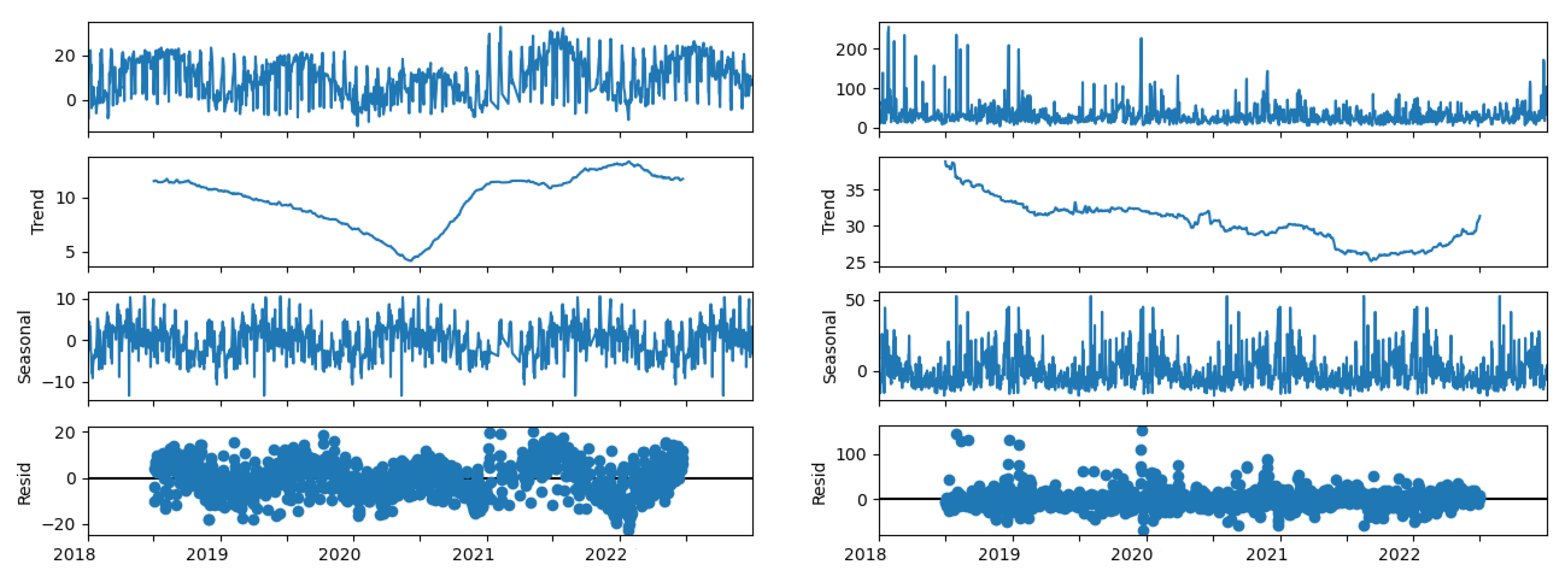
We begin with a straightforward examination of the data, noting that the five main stations provide daily averages for the period 2018–2022 and that there are another twenty stations placed in various locations for which we only have data for 2020. As Figure 4 shows, there is a clearly expressed seasonality (early cycles) and a downward trend in particulate matter pollution. The downward trends in pollution levels are better explained by warmer winters and stronger winds in the last years of the study period [58,59]. The COVID-19 pandemic had significant consequences, especially during the first lockdown between March and June 2020. Later rebounds were also observed, especially in some months of 2021 and 2022, due to the relatively short lockdowns in the country and the high elasticity of economic activity between them and after the periods of restrictions.
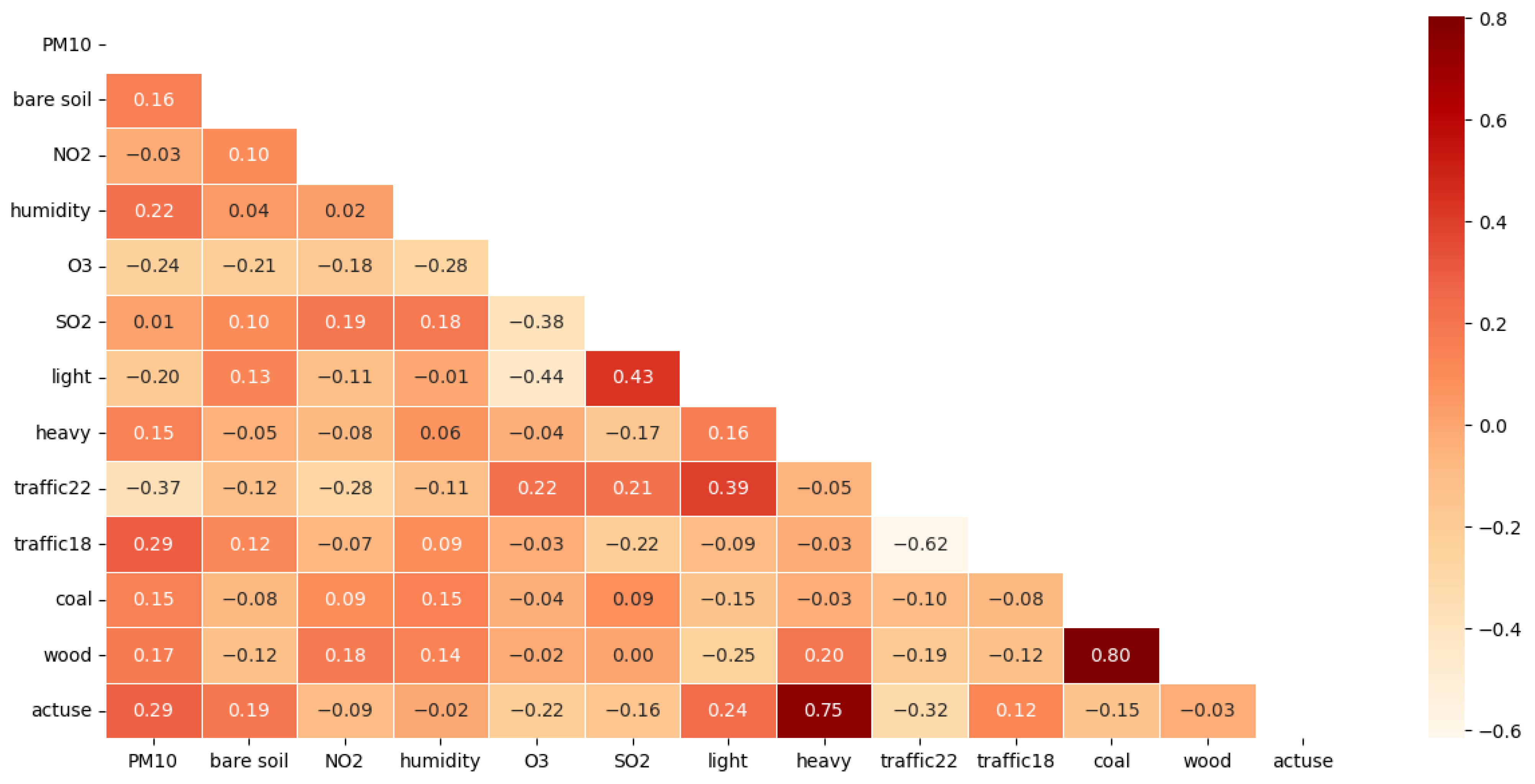
We also note that the meteorological parameters may vary greatly even for nearby stations, as is the case with wind speed. Sofia is located in a complex terrain and has a distinct urban morphology, which affects the microclimatic conditions in different areas of the city. We use both meteorological observations and pollutant concentration data that correspond to local wind conditions. This heterogeneity is taken into account by the models and should not affect the overall results. The correlation matrix is illustrated in Figure 3. Note the relatively high correlation between PM10 and NOX levels (which account for both NO and NO2) that is confirmed in the feature importance analysis for our models.
Elementary time series analysis reveals a clear pattern of seasonality in the PM10 levels, emphasized more in some locations than in others (see Figure 4), which has to do with the prevalence of meteorological factors. In the example above, we see distinct maxima in the warm and dry season for the station in Mladost district, while for the one in Hipodruma these maxima seem to be shifted to the cold and wet period. The explanation can be found in the significant micro-climate variations in the territory of Sofia Municipality: while the former area is open and windy, and thus a large part of its aerosol PM10 (which is low compared to other parts of the city) is attributed to resuspension, for the latter, traffic and heating play an essential role. Also, clearly, the signal-to-noise ratio and their amplitudes are quite different, as well as the trends: we see a clear downward trend in Mladost for the period 2018–2020, followed by a sharp re-bounce, while for Hipodruma both the decrease and increase of emissions are much more gradual, and the minimum is in 2021. This diversity makes it much harder to generalize the results. In any case, since both seasonality and long-term trend play a major role, our models reach higher evaluation metrics, in particular R 2 , when trained taking account of the date: it explains much of the variance by capturing the temporal dynamics, but since all the other features are spatially distributed, in the end we exclude it from the regression model.
Figure 4. Seasonality and trend in the PM10 levels from Mladost (left) and Hipodruma station (right).
Applsci 15 12783 g004

3.2. Data Pre-Processing

In order to achieve a meaningful result with just about a thousand data instances, we need to invest some effort in pre-processing. Firstly, we exclude features that have missing values above 10 % , such as wind speed and direction or air temperature (Table 1 shows the data after that has been done). The remaining gaps are quite manageable and can be dealt with using a simple proximity-based imputation method like KNN, for example. However, in this analysis we strive for high precision with limited resources, so a better choice would be the MICE (multiple imputation by chained equations) algorithm. It is somewhat more complex, but it takes into account the subtle relation between different features. After having tried both the KNN imputer with optimized number of neighbors k = 7 and MICE with BayesianRidge estimator, we chose to simply exclude rows having missing values (thus losing about 8.9 % of the data) as the inaccuracies they introduce contaminate the models.

3.3. Synthetic Data Generation

Here we also use the Gaussian Copula Synthesizer (GCS) to generate artificial data following the statistical distribution and inter-feature relations encoded in the raw data. It is a robust method using integral transforms based on the normal distribution. Data scientists often use it for their models, as it tends to preserve the correlations between features, which is important in studies like this (see, for example, [60,61]).
Finally, we need to take care of the data imbalances, in particular those in the bare soil area estimates, where almost 70 % of the instances are associated with no such spots within the buffer. Hence, the regression algorithm cannot ‘learn’ much from them. In order to do that, we use a famous algorithm known as SMOTER (synthetic minority oversampling technique for regression). Unlike conventional methods like bootstrapping which introduce bias in imbalanced data, SMOTER generates artificial data providing more instances of the underrepresented class, e.g., measurements near to bare soil surfaces. After applying the SMOTER algorithm, their share in the data set almost doubles—from 30.5 % to 59.3 % —although it does not target this specific feature but instead aims at all imbalances in the data. Apart from that, the synthetic minority oversampling increases its total volume from 1115 to 1689 instances, which is more than a 51 % increase, providing our regression models with a much better learning opportunity. In an alternative scenario, we include two more features (NO2 and sun radiation) while losing data rows due to missing values, in which case the model has to deal with only 875 instances. Note, also, that it is designed specifically not to introduce additional bias in the system and thus to minimize the risk of overfitting, which cannot be ignored if we use a more conventional technique such as bootstrapping. For further details on GCS and SMOTER we refer the reader, respectively, to [61,62].

3.4. Principal Component Analysis

Once the data is relatively balanced, we proceed to applying principal component analysis (PCA), which is often used as a dimensionality reduction technique, but in our case we need it purely for orthogonalization (for a comprehensive introduction to PCA with applications, we refer to [63]). This is important due to the relatively high correlations (Figure 3), which make it hard to assess the contribution of each individual feature to the predicted value of the target variable: e.g., if both sun radiation and humidity influence resuspension, but at the same time they are mutually entangled, so is their contribution to the process. To deal with this issue, PCA finds a canonical basis for the covariance matrix, in which it is diagonal, and the new features are the mutually orthogonal (e.g. non-correlated) eigenvectors, called principal components. They are ordered according to the magnitude of the corresponding eigenvalue, which yields the explained variance attributed to that particular component and, because of orthogonality, is not affected by the others. That particular feature of PCA is our main motivation to invoke it here, while the reduction argument is that as we reach some satisfactory level of explained variance, e.g., 85–95%, there is no practical point in adding more components, which allows us to work effectively with fewer features. Note also that PCA has the benefit of scaling the data, which is important for some algorithms, such as artificial neural networks, as well as eliminating multicollinearity that causes issues in linear models. Here we use neither of those, so these otherwise helpful features play no role in our analysis. Finally, it is important to note that along with its many advantages, PCA makes our task slightly more complicated: since the principal components are linear combinations of different features, interpreting the model is not so straightforward and one either has to invent new concepts or transform back to the original features, as we did. However, ‘bare soil’ happens to be almost identical with one of the components, namely PC4 (see Figure 5), so the contributions of the two overlap significantly. In the end, let us note that outliers are also kept, for the sake of generality: one meteorological station (Kopitoto) is outside the urban area and shows a different pattern.

3.5. Machine Learning Modeling

Next, we use several machine learning algorithms to build an acceptable regression model targeting the PM10 levels and then perform feature importance and SHAP analysis to assess the contribution of bare soil muddy patches in the resuspension of particulate matter, taking into account the previously obtained PMF results mentioned above [46]. We first use extreme gradient boosting, a standard ensemble learning model used extensively for both regression and classification problems. It yields high accuracy as long as we use all the available data. However, the satellite images are only accessible for certain days (cloudless days, etc.), and thus the number of rows in our filtered dataset is reduced from several thousand to several hundred. Consequently, more advanced methods are needed to perform a meaningful analysis in this case.
For this task, we resort to Amazon’s AutoGluon module, equipped with automated hyperparameter tuning, capabilities for multimodal machine learning and stacking of algorithms. Here we use mostly the latter, although AutoML is desirable if only for convenience. The idea behind stacking is essentially training multiple models on the dataset, ranking them according to their performance and then combining the best ones into a weighted ensemble (WE) meta-model. This can be done over and over again, hierarchically, and thus we speak of multi-level stacking, e.g., WE_L2 uses the predictions of WE_L1 as input data. This process increases the accuracy and reduces overfitting, but at a non-trivial computational cost. Additionally, after a few iterations, it naturally exhausts its ‘super powers’, so we never go beyond WE_L3: even WE_L2 performs quite well (Table 2).
Our base model uses the remaining 1115 data instances from real measurements, after removing the rows having missing values, and these data instances are then fed to a stacked ensemble regressor reaching a coefficient of determination R 2 0.8 ; or, alternatively, we can use data from only one of the platforms, which introduces some additional features, namely NO levels and sun radiation, but cuts the volume in half (563 instances). Therefore, model0 in our study corresponds to the former setting (with R 2 0.8 ), while model2 represents the latter, only with GCS and SMOTER in the pre-processing phase, to ensure more volume and improve the balance. Similarly, model1 is simply model0 using a SMOTER-balanced training set. The volume here is sufficient, but balancing via over-representation still adds around 40 % of the data. Finally, model1 and model2 are both supplemented by PCA in the pre-processing phase in order to separate the features better (eliminate multicollinearity) and assess the contribution of the new features independently. It turns out that for our dataset the ‘bare soil’ feature is almost coincident with one of the components (PC4) due to its relatively low correlations with the other features, and the corresponding SHAP values are quite close.

3.6. Feature Importance Analysis

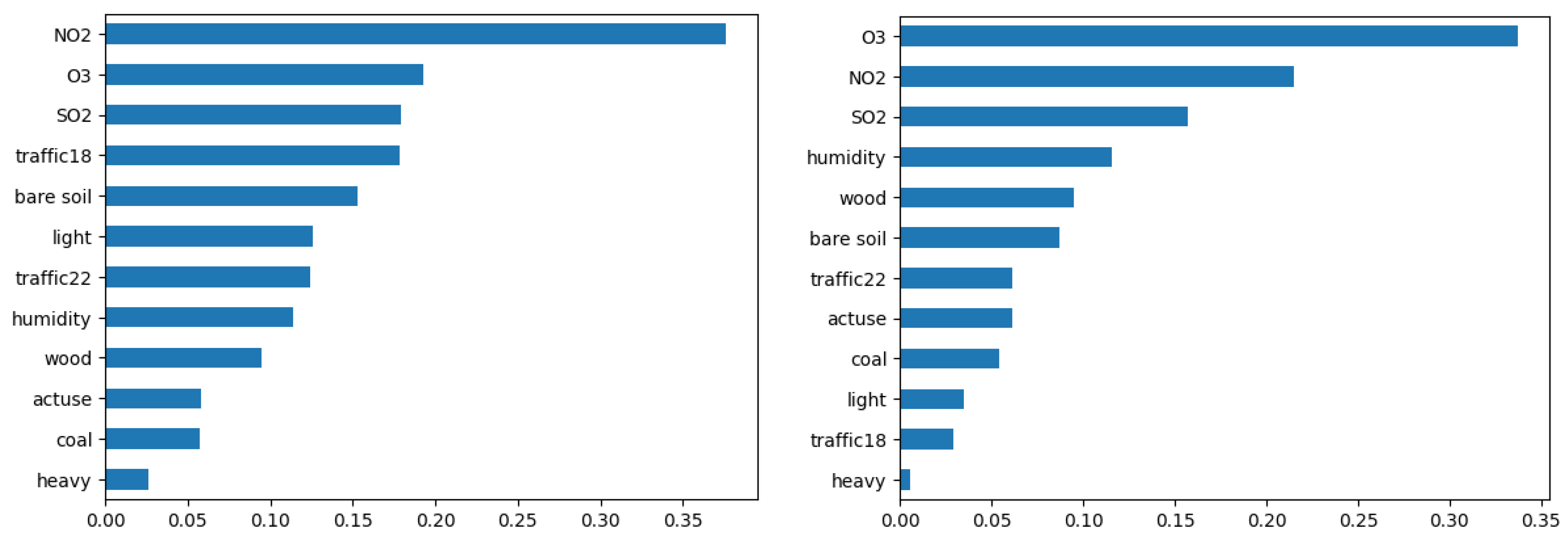
It is worth mentioning that the top performers in AutoGluon’s leaderboard are all based on ensemble learning: Random Forest, CatBoost, LightGBM, etc. Neural networks rank much lower. Of course, we ran multiple tests using different strategies, but for our best attempts the coefficient of determination stabilizes at R 2 0.9 , so before evaluating the contribution of bare soil surfaces, we need to take into account that our models explain only about 90 % of the target variable’s variance in the best case scenario. This makes all assessments quite rough, but we can still infer much: e.g., in optimally performing algorithms the bare soil contribution is below the middle and certainly after that of chemical compounds. In worse performing models it appears close to the top of the chart. Numerically, the feature importance for bare soil surfaces and PC4 varies between 0.05 and 0.2 (see Table 3 and Figure 6) while that of the leading feature (chemical compounds or traffic) reaches 0.3 and higher. Although one cannot directly link that number to causality, such a significant and persistent difference clearly indicates a stronger dependence for the PM pollution on human activities (industrial, traffic and heating) compared to natural sources of resuspension, with the possible exclusion of the regular transportation of Saharan dust.
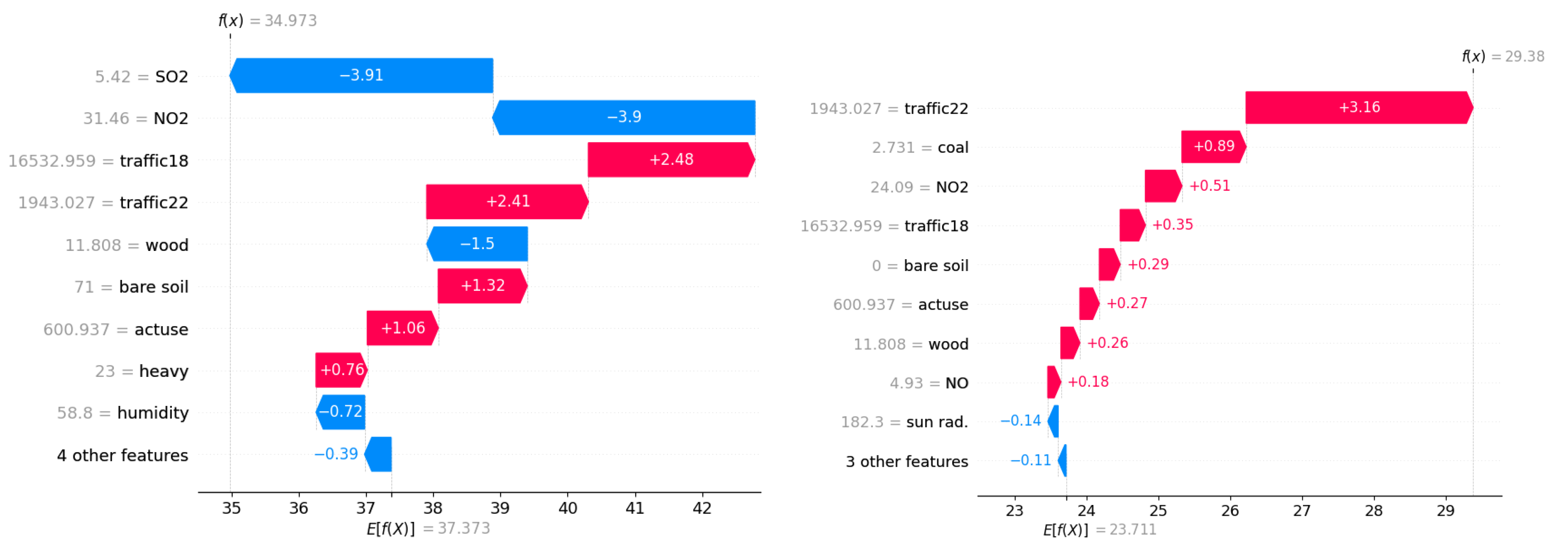
Another way to measure the contribution to the model is by running it with zero values for the corresponding feature and comparing the average for the predicted target variable (see Table 2). For the bare soil surfaces in particular, this yields a difference within the range of 1–4% and around 2.5 % for the best performing models. Taking into account also the conclusion of the chemical analysis [46] cited above, showing that resuspension contributes approximately 25 % of the total amount of aerosol PM10, we end up with a rough estimate of the contribution of bare soil surfaces to this process (and in that particular environment) with a ratio close to 10 % . Considering the heavy traffic, large number of active industrial and construction sites, and still quite common use of wood and coal stoves in the city, it is not hard to explain it, especially with the high correlations between particulate matter levels and chemical pollutants. However, that is more of a heuristic estimate than a precise calculation, since it is quite difficult to determine the confidence interval for that number: it could be quite large, although based on the model predictions we assume 5–15%, which agrees with the findings of similar studies for other urban areas, using different methods, but arriving at roughly the same prediction [64,65,66,67]. Finally, a third option is to use SHAP analysis, which shows among other things the effect each feature has on the average target value. An illustration is presented in Figure 7, with two waterfall charts representing the net effect of each feature on the target value.
Note that the SHAP estimate for ‘bare soil’ reaches the upper boundary of the interval determined by our naive approach, but Shapley values are expected to overshoot in the presence of multicollinearity, as is the case here. On the other hand, PCA-adjusted features, which eliminate this problem, hit the lower boundary, which is a common effect of the method, due to correlation spreading and scaling. Moreover, the interval 1–4% has been consistently confirmed by multiple experiments for that particular feature, while varying in quite a wide range for most others, thus making analogous estimates utterly unreliable in general.

4. Discussion

In this study, we consider a complex regression meta-model targeting PM10 aerosol levels, based on various features, including chemical compounds, humidity, estimated spatial distribution of the mean annual daily averaged traffic, wood and coal stoves, etc. With explained variance R 2 0.9 , SHAP and PCA analysis on the data in this study estimated that there is roughly a 5–15% contribution by bare soil areas to resuspension, and between 1 % and 4 % to the total PM10 levels. In comparison, factors such as resuspension due to traffic and wind blow or domestic heating may contribute up to 25–30% on seasonal bases according to previous studies [46], which is confirmed by the national report on the state and protection of the environment in the republic of Bulgaria [49] and other studies [6,7,68]. Features related to functional analysis, pollution inventory and chemical compounds in the atmosphere are highly correlational and used here only as a proxy to a different, hidden contributing factor. In any case, these numbers are, of course, preliminary and as mentioned before, the confidence interval is difficult to assess. Furthermore, the role of traffic in both mechanical distribution of mud and dispersion of deposited dust from all sources combined is a challenging linkage to be more precisely examined in the case of Sofia, again in relation to atmospheric conditions. This phenomenon requires more detailed in situ sampling and specific measurements and observations due to the large variance of parking and road surface conditions across the city space. The less-known role of muddy water runoff from poorly maintained terrains to parking and street surfaces, followed by drying and dispersion of the deposits, as well as the parallel leaf fall of street green, garden and park trees, and urban forests and the transformation of that biomass to wet or dry organic matter and its decomposition into dust throughout late autumn and winter, requires further investigation.
The main limitation in our study comes from the low spatial resolution of the available data, which also happens to contain a large portion of unreliable and missing values. That leads to the second issue: the dependence on modeled and interpolated data, as well as early averages being used as input data along with time-specific measurements, so the error propagates through the process, and on top of that we add synthetic data and oversampling using GCS and SMOTER. Although stacking ensemble learning algorithms allows us to build a fairly decent regression model even under these circumstances, the discrepancy surely may compromise our confidence in evaluating the contribution of a particular feature to the result. One way to address this is to conduct a large number of numerical experiments and apply standard statistical analysis on the resulting estimates. However, this is a time-consuming strategy even for a relatively small data set. That is why we use both different models and different estimates (naive, SHAP-based and PCA-aided) to obtain a rough preliminary assessment, meant to be further refined through more subtle analysis that we plan to conduct in future studies. A much better long-term solution is, of course, gathering more high-quality and diverse data, covering both temporal and spatial resolution criteria for a precise study, which is unfortunately in short supply in the region, even when an EU country capital is concerned. Bulgaria, along with other Balkan states, falls behind the trend for reliable and transparent real-time air quality monitoring, which is partly a reason for the excessive pollution-related mortality, respiratory diseases and overall reduced quality of life [51,69]. Moreover, the lack of reliable data impedes public awareness on actual risks and thus the pressure for solutions, which is a systemic problem for large urban populations.
The methods used in the study can be replicated in other cities and countries having similar problems related to higher proportions of bare soil surfaces, wet or dry, more contrasting seasons with stress on vegetation cover, low capacity for the increasing levels of motorization, illegal parking in public places and less coverage of open spaces with higher standards of public works. Southeastern Europe, the Middle East and many developing countries in the Global South can apply and adapt the approach. Meteorological and satellite imagery data are more universal, but census and cadastral data as well as traffic counts and statistical models are also easily accessible. If they are difficult to access, they can be replaced by more approximate but still relatively high-resolution datasets, such as the Global Human Settlement layers [70].

5. Conclusions

The present study suggests an approach to evaluate the contribution of bare soil areas to the resuspension of PM10 in an urban environment. For Sofia city, in particular, our results show around 10 % (between 5 % and 15 % ). Applied new techniques within a broader methodological framework focused on the specific needs of urban planning in the city to support decision-making at the local level. The actual air quality program of Sofia includes a set of at least five measures dedicated to reduce resuspension by inventory and mud patches through re-vegetation of undeveloped urban areas and voids, while also aiming to enforce vehicle parking bans in green areas [71].
There is no publicly available inventory yet, and the proposed approach may be helpful for more in-depth remote mapping and assessment of key areas to be addressed in the future, especially if combined with dispersion modeling and specific simulations. The measure is already being implemented, but without transparent prioritization and mostly based on random visual on-site inspections. Our study could be beneficial as a tool for supporting planning and decision-making, given the limited local resources and the vast number of urban surfaces in Sofia that still need to be inspected and regenerated. Additional selection criteria could be applied in relation to the population density and occupations, and the volume of traffic associated with some of the muddy patches, as well as their status in terms of ownership and designations in the local detailed development plans.
More direct and specific public health benefits will be further analyzed in future studies of multiple sources with their interactions and impacts. Well-targeted effective reduction of bare soils that represent muddy and/or dusty patches driven by natural and anthropogenic factors contributing to atmospheric resuspension of PM is manageable. Investment in public activities, better urban landscape, transport design and regulation could have a significant impact on public health, as nearly a quarter of PM10 is attributed to resuspension, and the majority of phenomena are related to local background sources and mechanical processes.

Author Contributions

Conceptualization, R.D. and A.B.; methodology, D.B., E.H. and A.B.; software, D.B. and E.H.; validation, D.B. and A.B.; formal analysis, D.B. and R.D.; investigation, D.B., A.B. and R.D.; resources, L.D., P.A.-K., E.H. and S.G.; data curation, A.B., L.D., P.A.-K., E.H. and S.G.; writing—original draft preparation, D.B., A.B. and R.D.; writing—review and editing, D.B. and R.D.; visualization, D.B.; supervision, A.B. and R.D.; project administration, R.D.; funding acquisition, R.D. All authors have read and agreed to the published version of the manuscript.

Funding

Reneta Dimitrova gratefully acknowledges the support provided by the UNITe project BG16RFPR002-1.014-0004, funded by PRIDST. The time devoted to this publication by D. Brezov, A. Burov, L. Dimova, S. Georgiev and E. Hristova was funded by the Bulgarian National Science Foundation (BNSF), under the project “Development of a methodology for assessing air quality and its impact on human health in urban environments”, grant number KΠ-06-H54/2.

Data Availability Statement

The raw data used in this study is publicly available and may be retrieved from Bulgaria’s system for informing the population about the quality of atmospheric air, on the webpage of the Executive Environment Agency (EEA) https://eea.government.bg/kav (accessed on 23 June 2025), as well as the Copernicus platform that gives access to the Sentinel-2 satellite image database https://dataspace.copernicus.eu/explore-data/data-collections/sentinel-data/sentinel-2 (accessed on 23 June 2025). The already processed data and predictions from previous models can be found in the cited literature, e.g., [46,52].

Conflicts of Interest

The authors declare no conflicts of interest.

Abbreviations

The following abbreviations are used in this manuscript:
NDVINormalized Difference Vegetation Index
NDMINormalized Difference Moisture Index
BSIBare Soil Index
PMparticulate matter
POIPoints Of Interest
AQSair quality station
SAsource appointment
PMFpositive matrix factorization
KNNk nearest neighbors (imputation)
MICEmultiple imputation by chained equations
GCSGaussian Copula Synthesizer
SMOTERsynthetic minority oversampling technique for regression
PCAprincipal component analysis
XGBoostextreme gradient boosting
WE_L2/L3level two/three weighted ensemble meta-models

References

  1. Romero-Lankao, P.; Dodman, D. Cities in Transition: Transforming Urban Centres from Hotbeds of GHG Emissions and Vulnerability to Seedbeds of Sustainability and Resilience: Introduction and Editorial Overview. Curr. Opin. Environ. Sustain. 2011, 3, 113–120. [Google Scholar] [CrossRef]
  2. World Health Organization. Air Pollution. In Compendium of WHO and Other UN Guidance on Health and Environment; World Health Organization: Geneva, Switzerland, 2022; Available online: https://www.urbanagendaplatform.org/sites/default/files/2023-04/WHO-HEP-ECH-EHD-22.01-eng.pdf (accessed on 23 June 2025).
  3. Oke, T.R.; Mills, G.; Christen, A.; Voogt, J.A. Urban Climates; Cambridge University Press: Cambridge, UK, 2017. [Google Scholar] [CrossRef]
  4. Lonati, G.; Crippa, M.; Gianelle, V.; Van Dingenen, R. Daily patterns of the multimodal structure of the particle number size distribution in Milan, Italy. Atmos. Environ. 2011, 45, 243–2442. [Google Scholar] [CrossRef]
  5. EEA. Air Quality in Europe—2019 Report; Publications Office of the European Union: Luxembourg, 2019; Available online: https://www.eea.europa.eu/en/analysis/publications/air-quality-in-europe-2019 (accessed on 23 June 2025).
  6. Petit, J.E.; Pallarés, C.; Favez, O.; Alleman, L.Y.; Bonnaire, N.; Rivière, E. Sources and geographical origins of PM10 in Metz (France) using oxalate as a marker of secondary organic aerosols by positive matrix factorization analysis. Atmosphere 2019, 10, 370. [Google Scholar] [CrossRef]
  7. Pio, C.; Alves, C.; Nunes, T.; Cerqueira, M.; Lucarelli, F.; Nava, S.; Calzolai, G.; Gianelle, V.; Colombi, C.; Amato, F.; et al. Source apportionment of PM2.5 and PM10 by Ionic and Mass Balance (IMB) in a traffic-influenced urban atmosphere, in Portugal. Atmos. Environ. 2020, 223, 117217. [Google Scholar] [CrossRef]
  8. Thorpe, A.; Harrison, R.M. Sources and properties of non-exhaust particulate matter from road traffic: A review. Sci. Total Environ. 2008, 400, 270–282. [Google Scholar] [CrossRef] [PubMed]
  9. Guttikunda, S.K.; Calori, G. A GIS based emissions inventory at 1 km × 1 km spatial resolution for air pollution analysis in Delhi, India. Atmos. Environ. 2013, 67, 101–111. [Google Scholar] [CrossRef]
  10. Faber, P.; Drewnick, F.; Borrmann, S. Aerosol particle and trace gas emissions from earthworks, road construction, and asphalt paving in Germany: Emission factors and influence on local air quality. Atmos. Environ. 2015, 122, 662–671. [Google Scholar] [CrossRef]
  11. Yan, H.; Li, Q.; Feng, K.; Zhang, L. The characteristics of PM emissions from construction sites during the earthwork and foundation stages: An empirical study evidence. Environ. Sci. Pollut. Res. 2023, 30, 62716–62732. [Google Scholar] [CrossRef]
  12. Charron, A.; Polo-Rehn, L.; Besombes, J.-L.; Golly, B.; Buisson, C.; Chanut, H.; Marchand, N.; Guillaud, G.; Jaffrezo, J.-L. Identification and quantification of particulate tracers of exhaust and non-exhaust vehicle emissions. Atmos. Chem. Phys. 2019, 19, 5187–5207. [Google Scholar] [CrossRef]
  13. Singh, V.; Srivastava, R.K.; Bhatt, A.K. Major Air Pollutants. In Battling Air and Water Pollution; Springer: Singapore, 2025. [Google Scholar] [CrossRef]
  14. Kupiainen, K.K.; Tervahattu, H.; Räisänen, M.; Mäkelä, T.; Aurela, M.; Hillamo, R. Size and composition of airborne particles from pavement wear, tires, and tractor sanding. Environ. Sci. Technol. 2005, 39, 699–706. [Google Scholar] [CrossRef]
  15. Norman, M.; Johansson, C. Studies of some measures to reduce road dust emissions from paved roads in Scandinavia. Atmos. Environ. 2006, 40, 6154–6164. [Google Scholar] [CrossRef]
  16. Casotti Rienda, I.; Alves, C.A. Road dust resuspension: A review. Atmos. Res. 2021, 261, 105740. [Google Scholar] [CrossRef]
  17. Denby, B.R.; Kupiainen, K.J.; Gustafsson, M. Chapter 9—Review of Road Dust Emissions. In Non-Exhaust Emissions; Amato, F., Ed.; Academic Press: Oxford, UK, 2018; pp. 183–203. [Google Scholar] [CrossRef]
  18. Amato, F.; Pandolfi, M.; Viana, M.; Querol, X.; Alastuey, A.; Moreno, T. Spatial and chemical patterns of PM10 in road dust deposited in urban environments. Atmos. Environ. 2009, 43, 1650–1659. [Google Scholar] [CrossRef]
  19. Yarmoshenko, I.; Malinovsky, G.; Baglaeva, E.; Seleznev, A. A Landscape Study of Sediment Formation and Transport in the Urban Environment. Atmosphere 2020, 11, 1320. [Google Scholar] [CrossRef]
  20. Chen, Z.; Chen, D.; Zhao, C.; Kwan, M.; Cai, J.; Zhuang, Y.; Zhao, B.; Wang, X.; Chen, B.; Yang, J.; et al. Influence of Meteorological Conditions on PM2.5 Concentrations Across China: A Review of Methodology and Mechanism. Environ. Int. 2020, 139, 105558. [Google Scholar] [CrossRef] [PubMed]
  21. Talepour, N.; Birgani, Y.T.; Kelly, F.J.; Jaafarzadeh, N.; Goudarzi, G. Analyzing Meteorological Factors for Forecasting PM10 and PM2.5 Levels: A Comparison between MLR and MLP Models. Earth Sci. Inform. 2024, 17, 5603–5623. [Google Scholar] [CrossRef]
  22. Huang, Y.; Cai, Y.; Jiao, J.; Pan, C.; Wang, G.; Li, C.; Jia, Z.; Chen, Z.; Zhou, Y.; Zhou, G. The Impact of Meteorological Factors and Canopy Structure on PM2.5 Dynamics Under Different Urban Functional Zones in a Subtropical City. Forests 2025, 16, 479. [Google Scholar] [CrossRef]
  23. Zhao, C.; Lin, Z.; Yang, L.; Jiang, M.; Qiu, Z.; Wang, S.; Gu, Y.; Ye, W.; Pan, Y.; Zhang, Y.; et al. A Study on the Impact of Meteorological and Emission Factors on PM2.5 Concentrations Based on Machine Learning. J. Environ. Manag. 2025, 376, 124347. [Google Scholar] [CrossRef] [PubMed]
  24. Liu, R.; Wang, M.; Chen, S.; Zhang, J.; Jin, X.; Ren, Y.; Chen, J. Historical Pollution Exposure Impacts on PM2.5 Dry Deposition and Physiological Responses in Urban Trees. Forests 2024, 15, 1614. [Google Scholar] [CrossRef]
  25. Tian, Y.; Zhang, L.; Wang, Y.; Song, J.; Sun, H. Temporal and Spatial Trends in Particulate Matter and the Responses to Meteorological Conditions and Environmental Management in Xi’an, China. Atmosphere 2021, 12, 1112. [Google Scholar] [CrossRef]
  26. Huber, M.; Welker, A.; Helmreich, B. Critical Review of Heavy Metal Pollution of Traffic Area Runoff: Occurrence, Influencing Factors, and Partitioning. Sci. Total Environ. 2016, 541, 895–919. [Google Scholar] [CrossRef]
  27. Brezonik, P.L.; Stadelmann, T.H. Analysis and Predictive Models of Stormwater Runoff Volumes, Loads, and Pollutant Concentrations from Watersheds in the Twin Cities Metropolitan Area, Minnesota, USA. Water Res. 2002, 36, 1743–1757. [Google Scholar] [CrossRef]
  28. Zhu, H.; Xu, Y.; Yan, B.; Guan, J. Snowmelt Runoff: A New Focus of Urban Nonpoint Source Pollution. Int. J. Environ. Res. Public Health 2012, 9, 4333–4345. [Google Scholar] [CrossRef]
  29. Westerlund, C.; Viklander, M. Particles and Associated Metals in Road Runoff During Snowmelt and Rainfall. Sci. Total Environ. 2006, 362, 143–156. [Google Scholar] [CrossRef]
  30. Hilliges, R.; Endres, M.; Tiffert, A.; Brenner, E.; Marks, T. Characterization of Road Runoff with Regard to Seasonal Variations, Particle Size Distribution and the Correlation of Fine Particles and Pollutants. Water Sci. Technol. 2017, 75, 1169–1176. [Google Scholar] [CrossRef] [PubMed]
  31. Furberg, A.; Arvidsson, R.; Molander, S. Dissipation of Tungsten and Environmental Release of Nanoparticles from Tire Studs: A Swedish Case Study. J. Clean. Prod. 2019, 207, 920–928. [Google Scholar] [CrossRef]
  32. Wang, Q.; Zhang, Q.; Dzakpasu, M.; Chang, N.; Wang, X. Transferral of HMs Pollution from Road-Deposited Sediments to Stormwater Runoff During Transport Processes. Front. Environ. Sci. Eng. 2019, 13, 13. [Google Scholar] [CrossRef]
  33. Doherty, S.J.; Dang, C.; Hegg, D.A.; Zhang, R.; Warren, S.G. Black Carbon and Other Light-Absorbing Particles in Snow of Central North America. J. Geophys. Res. Atmos. 2014, 119, 12807–12831. [Google Scholar] [CrossRef]
  34. Nazarenko, Y.; Fournier, S.; Kurien, U.; Rangel-Alvarado, R.B.; Nepotchatykh, O.; Seers, P.; Ariya, P.A. Role of Snow in the Fate of Gaseous and Particulate Exhaust Pollutants from Gasoline-Powered Vehicles. Environ. Pollut. 2017, 223, 665–675. [Google Scholar] [CrossRef]
  35. US EPA, Health and Environmental Effects of Particulate Matter (PM). Available online: https://www.epa.gov/pm-pollution/health-and-environmental-effects-particulate-matter-pm (accessed on 23 June 2025).
  36. Orellano, P.; Kasdagli, M.-I.; Pérez Velasco, R.; Samoli, E. Long-Term Exposure to Particulate Matter and Mortality: An Update of the WHO Global Air Quality Guidelines Systematic Review and Meta-Analysis. Int. J. Public Health 2024, 69, 1607683. [Google Scholar] [CrossRef]
  37. Health Effects Institute. State of Global Air 2024, a Special Report on Global Exposure to Air Pollution and Its Health Impacts, with a Focus on Children’s Health; Health Effects Institute; Boston, MA, USA, 2024; Available online: https://www.stateofglobalair.org/resources/archived/state-global-air-report-2024 (accessed on 23 June 2025).
  38. Weinmayr, G.; Romeo, E.; De Sario, M.; Weiland, S.K.; Forastiere, F. Short-term effects of PM10 and NO2 on respiratory health among children with asthma or asthma-like symptoms: A systematic review and meta-analysis. Environ. Health Perspect. 2010, 118, 449–457. [Google Scholar] [CrossRef]
  39. Dimitrova, R.; Lurponglukana, N.; Fernando, H.J.S.; Runger, G.C.; Hyde, P.; Hedquist, B.C.; Anderson, J.; Bannister, W.; Johnson, W. Relationship between particulate matter and childhood asthma–basis of a future warning system for central Phoenix. Atmos. Chem. Phys. 2012, 12, 2479–2490. [Google Scholar] [CrossRef]
  40. Pope, C.A., 3rd; Burnett, R.T.; Thun, M.J.; Calle, E.E.; Krewski, D.; Ito, K.; Thurston, G.D. Lung cancer, cardiopulmonary mortality, and long-term exposure to fine particulate air pollution. J. Am. Med. Assoc. 2002, 287, 1132–1141. [Google Scholar] [CrossRef]
  41. Neupane, B.K.; Acharya, B.K.; Cao, C.; Xu, M.; Bhattarai, H.; Yang, Y.; Wang, S. A systematic review of spatial and temporal epidemiological approaches, focus on lung cancer risk associated with particulate matter. BMC Public Health 2024, 24, 2945. [Google Scholar] [CrossRef]
  42. Global Burden of Cardiovascular Diseases and Risks 2023 Collaborators. Global, Regional, and National Burden of Cardiovascular Diseases and Risk Factors in 204 Countries and Territories, 1990–2023. J. Am. Coll. Cardiol. 2025, 86, 2167–2243. [Google Scholar] [CrossRef]
  43. Douwes, J.; Thorne, P.; Pearce, N.; Heederik, D. Bioaerosol health effects and exposure assessment: Progress and prospects. Ann. Occup. Hyg. 2003, 47, 187–200. [Google Scholar] [CrossRef]
  44. Rathnayake, C.M.; Metwali, N.; Baker, Z.; Jayarathne, T.; Kostle, P.A.; Thorne, P.S.; O’Shaughnessy, P.T.; Stone, E.A. Urban enhancement of PM10 bioaerosol tracers relative to background locations in the Midwestern United States. J. Geophys. Res. Atmos. 2016, 121, 5071–5089. [Google Scholar] [CrossRef]
  45. Yun, H.; Seo, J.H.; Kim, Y.-K.; Yang, J. Examining the bacterial diversity including extracellular vesicles in air and soil: Implications for human health. PLoS ONE 2025, 20, e0320916. [Google Scholar] [CrossRef] [PubMed]
  46. Hristova, E.; Veleva, B.; Georgieva, E.; Branzov, H. Application of Positive Matrix Factorization Receptor Model for Source Identification of PM10 in the City of Sofia, Bulgaria. Atmosphere 2020, 11, 890. [Google Scholar] [CrossRef]
  47. Delaney, B.; Tansey, K.; Whelan, M. Satellite Remote Sensing Techniques and Limitations for Identifying Bare Soil. Remote Sens. 2025, 17, 630. [Google Scholar] [CrossRef]
  48. Executive Environment Agency (EEA). System for Informing the Population About the Quality of Atmospheric Air. Available online: https://eea.government.bg/kav (accessed on 23 June 2025).
  49. Executive Environment Agency (EEA). National Report for the Condition and Preservation of the Environment: Pollutant Emissions and Quality of the Atmospheric Air. 2023. Available online: https://eea.government.bg/bg/soer/2024/1Air.pdf (accessed on 23 June 2025). (In Bulgarian)
  50. Burov, A.; Brezov, D. Transport Emissions from Sofia’s Streets—Inventory, Scenarios, and Exposure Setting. In Environmental Protection and Disaster Risks; Dobrinkova, N., Nikolov, O., Eds.; EnviroRISKs 2022: Lecture Notes in Networks and Systems; Springer: Cham, Switzerland, 2023; Volume 638. [Google Scholar] [CrossRef]
  51. Khomenko, S.; Burov, A.; Dzhambov, A.M.; de Hoogh, K.; Helbich, M.; Mijling, B.; Hlebarov, I.; Popov, I.; Dimitrova, D.; Dimitrova, R.; et al. Health Burden and Inequities of Urban Environmental Stressors in Sofia, Bulgaria. Environ. Res. 2025, 279, 121782. [Google Scholar] [CrossRef]
  52. Brezov, D.; Burov, A. Ensemble Learning Traffic Model for Sofia: A Case Study. Appl. Sci. 2023, 13, 4678. [Google Scholar] [CrossRef]
  53. Liu, X.; Zhang, X.; Jin, B.; Wang, T.; Qian, S.; Zou, J.; Dinh, V.N.T.; Jaffrezo, J.L.; Uzu, G.; Dominutti, P.; et al. Source Apportionment of PM10 Based on Offline Chemical Speciation Data at 24 European Sites. Npj Clim. Atmos. Sci. 2025, 8, 255. [Google Scholar] [CrossRef]
  54. Mircea, M.; Calori, G.; Pirovano, G.; Belis, C.A. European guide on air pollution source apportionment for particulate matter with source oriented models and their combined use with receptor models. In EUR 30082 EN; Publications Office of the European Union: Luxembourg, 2020; ISBN 978-92-76-10698-2. [Google Scholar]
  55. Hutter, F.; Kotthoff, L.; Vanschoren, J. Automated Machine Learning: Methods, Systems, Challenges; Springer: Berlin/Heidelberg, Germany, 2019; ISBN 9783030053185. [Google Scholar]
  56. Erickson, N.; Mueller, J.W.; Shirkov, A.; Zhang, H.; Larroy, P.; Li, M.; Smola, A. AutoGluon-Tabular: Robust and Accurate AutoML for Structured Data. arXiv 2020. [Google Scholar] [CrossRef]
  57. Ganaie, M.A.; Hu, M.; Malik, A.K.; Tanveer, M.; Suganthan, P.N. Ensemble Deep Learning: A Review. Eng. Appl. Artif. Intell. 2022, 115, 105151. [Google Scholar] [CrossRef]
  58. Gospodinov, I.; Tsenova, B. Some weather and climate facts for year 2020 in Bulgaria—Based on the Annual hydro-meteorological bulletin of NIMH. Bul. J. Meteo Hydro 2021, 25, 72–88. [Google Scholar]
  59. NIMH. The Changing Climate of Bulgaria—Data and Analyses; Marinova, T., Bocheva, L., Eds.; NIMH: Sofia, Bulgaria, 2023; ISBN 978-954-90537-3-9. (In Bulgarian). Available online: https://www.meteo.bg/meteo7/sites/storm.cfd.meteo.bg.meteo7/files/kniga_klim_promeni_23-12-2023_KM_ff.pdf (accessed on 23 June 2025).
  60. Benali, F.; Bodénès, D.; Labroche, N.; de Runz, C. MTCopula: Synthetic complex data generation using copula. In Proceedings of the 23rd International Workshop on Design, Optimization, Languages and Analytical Processing of Big Data (DOLAP ‘21), Nicosia, Cyprus, 23 March 2021; pp. 51–60. [Google Scholar]
  61. Masarotto, G.; Varin, C. Gaussian Copula Marginal Regression. Electron. J. Statist. 2012, 6, 1517–1549. [Google Scholar] [CrossRef]
  62. Torgo, L.; Ribeiro, R.P.; Pfahringer, B.; Branco, P. SMOTE for Regression. In Progress in Artificial Intelligence, Proceedings of the 16th Portuguese Conference on Artificial Intelligence, EPIA 2013, Angra do Heroísmo, Portugal, 9–13 September 2013, Proceedings; Correia, L., Reis, L.P., Cascalho, J., Eds.; Lecture Notes in Computer Science; Springer: Berlin/Heidelberg, Germany, 2013; Volume 8154. [Google Scholar] [CrossRef]
  63. Jolliffe, I.T.; Cadima, J. Principal Component Analysis: A Review and Recent Developments. Philos. Trans. A Math. Phys. Eng. Sci. 2016, 374, 20150202. [Google Scholar] [CrossRef] [PubMed]
  64. Linda, J.; Uhlík, O.; Köbölová, K.; Pospíšil, J.; Apeltauer, T. Recognition of Wind-Induced Resuspension of PM10 and Its Fractions PM10-2.5, PM2.5-1, and PM1 in Urban Environments. Aerosol Sci. Technol. 2025, 59, 567–579. [Google Scholar] [CrossRef]
  65. Boga, R.; Keresztesi, Á.; Bodor, Z.; Tonk, S.; Szép, R.; Micheu, M.M. Source identification and exposure assessment to PM10 in the Eastern Carpathians, Romania. J. Atmos. Chem. 2021, 78, 77–97. [Google Scholar] [CrossRef]
  66. Linda, J.; Pospíšil, J.; Köbölová, K.; Ličbinský, R.; Huzlík, J.; Karel, J. Conditions Affecting Wind-Induced PM10 Resuspension as a Persistent Source of Pollution for the Future City Environment. Sustainability 2022, 14, 9186. [Google Scholar] [CrossRef]
  67. Karagulian, F.; Belis, C.A.; Dora, C.F.C.; Prüss-Ustün, A.M.; Bonjour, S.; Adair-Rohani, H.; Amann, M. Contributions to Cities’ Ambient Particulate Matter (PM): A Systematic Review of Local Source Contributions at Global Level. Atmos. Environ. 2015, 120, 475–483. [Google Scholar] [CrossRef]
  68. Lawrence, S.; Sokhi, R.; Ravindra, K.; Mao, H.; Prain, H.D.; Bull, I.D. Source apportionment of traffic emissions of particulate matter using tunnel measurements. Atmos. Environ. 2013, 77, 548–557. [Google Scholar] [CrossRef]
  69. Dzhambov, A.; Dimitrova, V.; Germanova, N.; Burov, A.; Brezov, D.; Hlebarov, I.; Dimitrova, R. Joint associations and pathways from greenspace, traffic-related air pollution, and noise to poor self-rated general health: A population-based study in Sofia, Bulgaria. Environ. Res. 2023, 231, 116087. [Google Scholar] [CrossRef] [PubMed]
  70. Pesaresi, M.; Schiavina, M.; Politis, P.; Freire, S.; Krasnodębska, K.; Uhl, J.H.; Carioli, A.; Corbane, C.; Dijkstra, L.; Florio, P.; et al. Advances on the Global Human Settlement Layer by Joint Assessment of Earth Observation and Population Survey Data. Int. J. Digit. Earth 2024, 17, 2390454. [Google Scholar] [CrossRef]
  71. Comprehensive Program for Improving the Quality of Atmospheric Air of Sofia Municipality for the Period 2021–2026. Available online: https://www.sofia.bg/components-environment-air (accessed on 23 June 2025). (In Bulgarian).
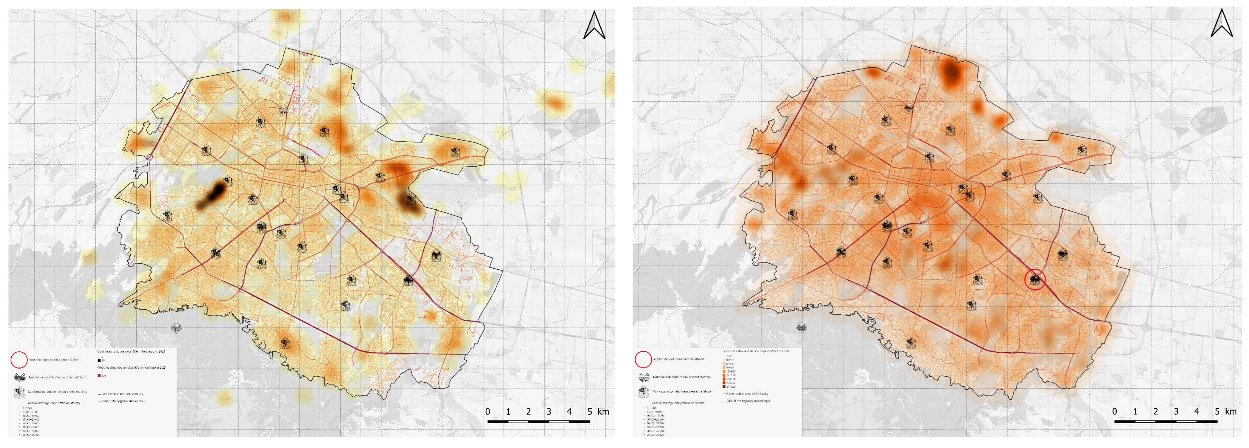
Figure 1. Heatmap illustrating the active wood/coal stoves distribution (left) and the BSI index (right), both including modeled traffic.
Applsci 15 12783 g001
Figure 2. Merging and stacking of multiple models in AutoML.
Applsci 15 12783 g002
Figure 3. Correlation matrix of the regression model features (raw data).
Applsci 15 12783 g003
Figure 5. PCA weight diagram, showing relations between features and components (left) and cumulative explained variance (right).
Applsci 15 12783 g005
Figure 6. Feature importance evaluation for model0 (left) and model2 (right) according to AutoGluon’s Weighted Ensemble Level 3.
Applsci 15 12783 g006
Figure 7. SHAP waterfall diagrams for a straightforward (left) and a PCA-aided model (right) confirming the limits 1–4% in Table 3.
Applsci 15 12783 g007
Table 1. Description of the input data.
FeatureData DescriptionMissing
PM10aerosol d 10 μm particulate matter levels (daily average) 3.8 %
NO2aerosol nitrogen dioxide concentration (daily average) 3.5 %
SO2aerosol sulfur dioxide concentration (daily average) 1.7 %
O3aerosol ozone concentration (daily average) 2.0 %
humidityair humidity (daily average) 6.6 %
bare soilestimated area of bare soil spots within a r = 250 m radius (based on satellite data)-
sun rad. 1sun radiation (daily average) 47.4 %
NO 1aerosol nitrogen oxide concentration (daily average) 45.4 %
actuseheatmap with r = 200 m of estimated motorized users (POI and cadastral data based)-
woodestimated density of wood stove user pixels within a r = 500 m radius-
coalestimated density of coal stove user pixels within a r = 500 m radius-
traffic18IDW-interpolated mean traffic spatial distribution model for 2018-
traffic22IDW-interpolated mean traffic spatial distribution model for 2022-
lightestimated contribution of light vehicles (cars) to the traffic-
heavyestimated contribution of heavy vehicles (trucks, etc.) to the traffic-
1 These particular features are only used in model2, which involves more parameters for fewer data sources.
Table 2. AutoGluon model ranking according to evaluation metric R 2 .
Modelmodel0model1model1 + PCAmodel2 + PCA
WeightedEnsemble_L3 0.805 0.891 0.892 0.896
ExtraTreesMSE_BAG_L2 0.800 0.890
RandomForestMSE_BAG_L2 0.792 0.886 0.891 0.895
CatBoost_BAG_L2 0.791 0.883 0.887 0.888
NeuralNetFastAI_BAG_L2 0.784 0.882
LightGBM_BAG_L2 0.788 0.881 0.883 0.890
WeightedEnsemble_L2 0.800 0.880 0.879 0.860
Table 3. Feature importance assessment for the different models via feature ablation and effect.
Modelmodel0model1model2Mean Effect
NO2 0.376 0.171 0.215 7–11%
O3 0.193 0.311 0.338 18–23%
SO2 0.179 0.115 0.157 5–18%
actuse 0.058 0.233 0.061 4–7%
humidity 0.114 0.205 0.115 9–26%
bare soil 0.153 0.169 0.087 1–4%
coal 0.057 0.107 0.054 3–7%
wood 0.095 0.130 0.095 3–17%
traffic22 0.125 0.159 0.061 15–28%
traffic18 0.179 0.029 0.029 2–23%
heavy 0.026 0.067 0.006 2–5%
light 0.126 0.033 0.035 8–15%
Disclaimer/Publisher’s Note: The statements, opinions and data contained in all publications are solely those of the individual author(s) and contributor(s) and not of MDPI and/or the editor(s). MDPI and/or the editor(s) disclaim responsibility for any injury to people or property resulting from any ideas, methods, instructions or products referred to in the content.