Article

Hybrid Deep Learning Framework for Forecasting Ground-Level Ozone in a North Texas Urban Region

by
Jithin Kanayankottupoyil
1,
Abdul Azeem Mohammed
2 and
Kuruvilla John
1,*
1
Department of Mechanical Engineering, University of North Texas, 3940 North Elm Street, Denton, TX 76207, USA
2
Department of Computer Science and Engineering, University of North Texas, 3940 North Elm Street, Denton, TX 76207, USA
*
Author to whom correspondence should be addressed.
Appl. Sci. 2025, 15(22), 11923; https://doi.org/10.3390/app152211923
Submission received: 10 October 2025 / Revised: 31 October 2025 / Accepted: 3 November 2025 / Published: 10 November 2025
(This article belongs to the Special Issue Air Quality Monitoring, Analysis and Modeling)

Abstract

Ground-level ozone is a critical secondary air pollutant and greenhouse gas, especially in urban oil and gas regions, where it poses severe public health and environmental risks. Urban areas in North Texas have experienced persistently elevated ozone levels over the past two decades despite emission control efforts, highlighting the need for advanced forecasting tools. This study presents a hybrid recurrent neural network (RNN) model that combines Gated Recurrent Unit (GRU) and Long Short-Term Memory (LSTM) architectures to predict 8 h average ground-level ozone concentrations over a full annual cycle. The model leverages one-hour lagged ozone precursor pollutants (VOC and NOx) and seven meteorological variables, using a novel framework designed to capture complex temporal dependencies and spatiotemporal variability in environmental data. Trained and validated on multi-year datasets from two distinctly different urban air quality monitoring sites, the model achieved high predictive accuracy (R2 ≈ 0.97, IoA > 0.96), outperforming standalone LSTM and Random Forest models by 6–12%. Beyond statistical performance, the model incorporates Shapley Additive exPlanation (SHAP) analysis to provide mechanistic interpretability, revealing the dominant roles of relative humidity, temperature, solar radiation, and precursor concentrations in modulating ozone levels. These findings demonstrate the model’s effectiveness in learning the nonlinear dynamics of ozone formation, outperforming traditional statistical models, and offering a reliable tool for long-term ozone forecasting and regional air quality management.

1. Introduction

Tropospheric ozone is a significant secondary greenhouse gas and air pollutant that adversely affects climate, ecosystems, and human health. Exposure to elevated ozone concentrations impairs pulmonary and cardiovascular function, increases asthma incidence, and exacerbates respiratory conditions [1,2,3,4,5,6]. Additionally, ozone damages vegetation and reduces agricultural productivity, with global implications for food security [7,8]. Ground-level ozone is not directly emitted; it forms via photochemical reactions between nitrogen oxides (NOx) and volatile organic compounds (VOCs) under sunlight, and it undergoes titration by nitric oxide (NO) at night, creating nitrogen dioxide (NO2) [9,10,11].
Despite aggressive NOx and VOC emission reduction strategies, many urban regions, including North Texas, continue to experience chronic ozone non-attainment episodes, largely due to complex nonlinear atmospheric chemistry, local meteorological variability, and regional precursor transport. Predicting ozone concentrations in these environments remains challenging, particularly because ozone formation is influenced by interacting factors such as temperature, humidity, solar radiation, wind dynamics, and planetary boundary layer height.
Traditionally, ozone prediction models are classified into two types: deterministic and empirical models [12,13]. Deterministic models, such as chemical transport models (CTMs), employ numerical simulations to simulate physical and chemical processes that influence air pollutants, such as emission, transformation, dispersion, and transport [14,15,16,17]. However, these models often involve uncertainties due to process simplifications, hypotheses, and parameterizations [18,19,20]. These uncertainties can result in systematic inaccuracies between model predictions and actual measurements, such as incorrectly depicting the yearly ozone cycle or the effect of climatic factors such as solar radiation and humidity on ozone levels [21]. Furthermore, CTMs struggle to capture local events because of their coarse resolution [22,23,24] and are computationally intensive, making operational use time-consuming [25,26]. As a result, while deterministic models are effective for analyzing air quality on large scales, they are less accurate on smaller, more localized scales such as urban regions [22,23,27].
Empirical or statistical models are data-driven methods that predict output using statistical techniques. Linear regression is a basic form of these models, fitting data to a hyperplane but sometimes struggling to capture local variations and nonlinearities [28,29,30]. Instance-based algorithms like K-Nearest Neighbor (kNN) and Support Vector Machines (SVM) build predictions from local relationships, without depending on global rules [31,32,33].
Machine learning (ML) has significantly improved empirical models’ accuracy by handling nonlinearities and identifying patterns in air pollution and meteorological data. Traditional statistical models, including multiple linear regression (MLR) [34,35] and Multivariate Adaptive Regression Splines [36,37], have served as the foundation, while modern machine learning models such as Random Forest [37,38], Extreme Gradient Boosting (XGBoost) [39,40], Bayesian Network [41], and Support Vector Machine (SVM) have also been studied [33,41,42,43]. Recent studies have extensively compared various ML algorithms for predicting urban air pollution, particularly ozone. Elkamel et al. (2001) [28] used artificial neural networks, as well as nonlinear and linear regression models, to estimate ozone levels based on weather conditions and precursor concentrations during 60 days in Kuwait. For a study based in Saudi Arabia, Pan et al. (2023) [44] built and analyzed 19 machine learning models, including Random Forest and Gradient Boosting, with R2 values ranging from 0.82 to 0.99. The study used 1 h and 3 h lagged ozone concentration data. Juarez et al. (2022) [45] investigated eight machine learning models in Delhi, including XGBoost and Long Short-Term Memory (LSTM), for a 24 h ozone forecast and found R2 values ranging from 0.2 to 0.61. Lyu et al. (2022) [46] used Random Forest and Decision Tree Regression in the Beijing–Tianjin–Hebei region of China to forecast daily and monthly ozone levels over multiple years, with R2 values between 0.44 and 0.96. Capilla et al. (2016) [47] forecasted ozone levels for 1, 8, and 24 h ahead in an urban area along the eastern coast of the Iberian Peninsula, reporting that a Multi-Layer Perceptron network outperformed multiple linear regression. These ML models succeed at processing nonlinear data. However, they often fail in adequately addressing temporal dependencies. This drawback limits their efficacy in cases where forecasting future conditions based on historical and current data patterns is critical.
Deep learning (DL) methods are very effective in addressing temporal dependencies in predicting ozone concentrations, but they require careful setup and domain knowledge in model construction. The primary climatic parameters in predicting local fluctuations in ozone include temperature, relative humidity, wind speed, and solar radiation, all of which influence chemical reactions that alter ozone levels [48,49,50]. Weng et al. (2022) [51] recognized the importance of these factors in ozone dynamics, noting that their impact varies by region. Recent research supports the efficiency of deep learning for forecasting air pollutants. Chang et al. (2023) [52] forecasted air pollution levels in Beijing using several neural network architectures, including LSTM and Bidirectional LSTM (BiLSTM) models, attaining R2 values of 0.90–0.92. Ma et al. (2019) [39] and Antonio et al. (2019) [53] employed a hybrid CNN-LSTM model to forecast PM2.5, with RMSE values of 14.30 and 8.40, respectively. Furthermore, Ko et al. (2022) [54] created a BiLSTM model that uses planetary boundary layer data to forecast ozone concentrations for the next 24 h across numerous stations, with an RMSE ranging from 6.6 to 9.8.
This study addresses these knowledge gaps by developing a novel hybrid RNN framework combining GRU and LSTM layers to forecast ozone concentrations across multiple years and urban monitoring sites in North Texas. In this study, we explicitly focused on the following:
(1)
Integrating chemical precursors and meteorological drivers,
(2)
Incorporating one-hour lagged input variables to enhance temporal learning,
(3)
Providing mechanistic interpretability using SHAP analysis, and
(4)
Evaluating generalization performance across heterogeneous urban airsheds.
Unlike conventional short-term models, our hybrid approach is designed for year-long predictions, extending the forecasting horizon beyond prior studies. We perform comprehensive data exploration, including correlation analysis and temporal trend assessments, followed by model development and rigorous performance evaluation. By combining domain knowledge with state-of-the-art deep learning, this work contributes a scientifically robust and practically useful framework for long-horizon air quality forecasting, with applications in regulatory planning, public health, and climate adaptation.

2. Data and Methods

2.1. Data

This study focuses on two long-term ozone non-attainment sites in North Texas: Fort Worth Northwest (CAMS 013; 32°48′21″ N, 97°21′24″ W) and Dallas Hinton (CAMS 0161; 32°49′12″ N, 96°51′36″ W), both part of the Texas Commission on Environmental Quality (TCEQ) monitoring network. The geographical locations of the monitoring stations are shown in Figure 1. Both sites have recorded persistent ozone exceedances over the past two decades, influenced by urban activities, industrial emissions, and regional oil and gas operations [55,56].
We obtained hourly pollutant and meteorological data from the Texas Air Monitoring Information System (TAMIS), curated and managed by TCEQ. Specifically, we collected the following:
  • Air pollutants: ozone (ppb), NOx (ppb), and 26 individual VOC species (ppbV) measured by Automated Gas Chromatographs (AutoGC),
  • Meteorological parameters: outdoor temperature (OT, °F), peak wind gust (PWG, mph), relative humidity (RH, %), solar radiation (SR, W/m2), dew point temperature (DP, °F), resultant wind speed (WS, mph), and resultant wind direction (WD, degrees).
The CAMS 013 dataset spans from 1 January 2014 to 31 December 2023, while CAMS 0161 covers 1 January 2015 to 31 December 2019; the shorter duration at CAMS 0161 is due to the discontinuation of NOx measurements after 2019.
Exploratory analysis indicated a heavy right skew in precursor concentrations (NOx skewness = 4.02; VOCs skewness = 5.64; Table 1), which is typical of episodic, emission-driven regimes. To preserve the original physical scale and monotonic structure of precursor–ozone relationships—particularly at low concentrations where log transforms can distort small signals—we applied feature-wise Min–Max scaling (range [0, 1]) to all inputs and the target. Min–Max scaling bounds the dynamic range and stabilizes gradient-based optimization while retaining the raw rank ordering and relative spacing of observations. Because PCA can be sensitive to scale and centering, we performed PCA on the scaled features (seven components selected by elbow/cumulative variance), which primarily addresses multicollinearity among chemically related VOC groups and meteorological covariates.
To ensure input feature quality, we applied rigorous data preprocessing:
  • Among the 26 VOCs, we selected 22 species based on data completeness (>90% coverage) and feature importance analysis with respect to ozone, identified via SHAP.
  • Parameters with <10% missing data were gap-filled using temporal imputation (mean of the same date and time from neighboring years).
  • Parameters with >10% missing data were excluded.
  • Outlier retention was prioritized, recognizing that high ozone events and precursor spikes are critical for model learning in non-attainment areas.
Temporal trends were assessed for all variables (Section 2.3.1). While air pollutant concentrations showed no consistent linear or polynomial trends over the study period, several meteorological variables (e.g., OT, SR) exhibited gradual trends, reflecting underlying climatological shifts.
For model development, the CAMS 013 data were divided into training/validation (2014–2020) and testing (2021–2023) subsets, while CAMS 0161 data (2015–2019) were reserved entirely for out-of-sample generalization testing. We conducted SHAP analysis to quantify the contribution of each input feature to the model’s output and used correlation matrices to explore linear associations with ozone concentrations.
For this multiyear, a multisite dataset provides a rich foundation to evaluate not only predictive accuracy but also the model’s capacity to generalize across space, time, and meteorological regimes—a key advancement over prior studies limited to short-term, single-site predictions.

2.2. Methods

We utilized data from CAMS 013 (2014–2020) for model training and internal validation and evaluated model generalization on out-of-sample data from CAMS 013 (2021–2023) and high-ozone events at CAMS 0161 (2015–2019). This setup enabled rigorous evaluation of both temporal and spatial generalizability across multiple years and sites with distinct emission profiles. In designing the predictor inputs, we incorporated one-hour lagged values for ozone, NOx, VOCs, and key meteorological parameters—including OT, SR, WS, RH, PWG, DP, and WD. This decision was motivated by atmospheric chemistry principles: short-term variability in these parameters strongly influences photochemical ozone formation, titration, and dispersion processes.
The use of lagged variables is consistent with and expands upon prior studies. For example, Pan et al. (2023) [44] applied 1–3 h lagged ozone inputs for week-ahead forecasting; Wang et al. (2020) [57] used 24–168 h lagged data for 6–48 h predictions; Shah et al. (2024) [58] applied 2–4 h lagged ozone values for daily forecasts; and Álvaro et al. (2018) [59] utilized 24–28 h lags for next-day predictions. However, unlike these short- to medium-term approaches, our framework uniquely integrates one-hour lagged precursor and meteorological drivers for long-horizon (annual-scale) ozone forecasting, combining short-term memory and long-term pattern recognition within a hybrid deep learning architecture.
The inclusion of these immediate precursor signals enables the model to capture nonlinear feedback between recent atmospheric states and ozone production, improve responsiveness to sudden precursor emission changes, and maintain predictive stability over extended timescales by linking short- and long-range dependencies.
This methodological innovation—coupling fine-scale temporal dynamics with long-term generalization—is one of the key distinguishing features of our approach compared to existing empirical and deep learning ozone forecasting models. In this section, we describe the LSTM and GRU networks, which have been widely used for time series prediction studies.

2.2.1. Long Short-Term Memory (LSTM)

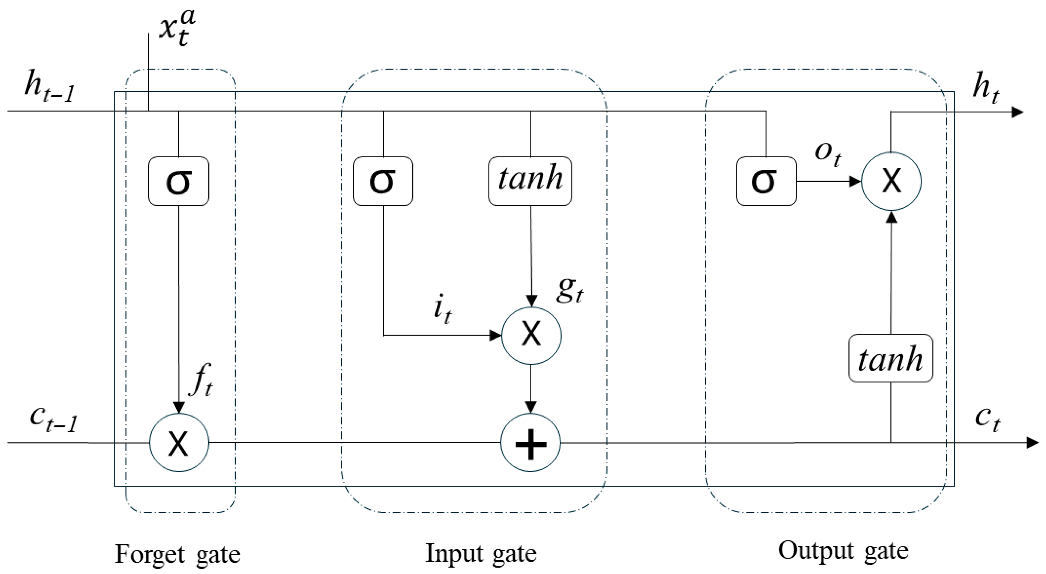
Long Short-Term Memory (LSTM) networks are a specialized form of recurrent neural networks (RNNs) developed to address the vanishing gradient problem that limits the ability of conventional RNNs to capture long-range temporal dependencies [60,61]. In standard RNNs, backpropagated gradients tend to decay or explode over long sequences, leading to the loss of information from earlier time steps. LSTMs overcome this by introducing a gated memory architecture that selectively regulates the retention, update, and output of information across time.
An LSTM unit consists of three principal gates:
  • Forget gate—Determines which information from the previous cell state to discard,
  • Input gate—Regulates which new information to add, combining a sigmoid filter with a tanh-generated candidate vector,
  • Output gate—Controls the portion of the updated cell state exposed as output to the next layer.
Figure 2 shows the LSTM model architecture. It has a forget gate f t , input node g t , input gate i t , output gate o t , and connection units. All the units and nodes can be expressed as follows:
f t = σ   W f x x t + W f h h t 1 + b f
i t = σ   W i x x t + W i h h t 1 + b i
g t =   W g x x t + W g h h t 1 + b g
o t = σ   W o x x t + W o h h t 1 + b o
c t = g t   i t + c t 1 f t
h t =   s t o t
where Wfx, Wfh, Wix, Wih, Wgx, Wgh, Wox, and Woh are weight matrices associated with respective network activation functions. bf, bi, bg, and bo are bias values. The operation denotes an element-wise multiplication. σ and φ denote the sigmoid and tanh activation functions, respectively.
The central element, the cell state (cₜ), serves as a conveyor of long-term dependencies, modulated at each step by the combined action of the forget and input gates. This dual mechanism allows LSTMs to maintain relevant historical patterns while discarding irrelevant or outdated information, making them highly effective for tasks requiring long-term sequence learning.
LSTMs have been widely applied in both sequence classification [62,63,64] and time series forecasting [65,66,67], including environmental modeling domains where pollutant concentrations are influenced by both immediate precursor conditions and accumulated meteorological histories. By enabling selective memory over extended sequences, LSTMs provide a mathematically robust solution for learning nonlinear dynamics in environmental time series data.

2.2.2. Gated Recurrent Unit (GRU)

The Gated Recurrent Unit (GRU) is a streamlined recurrent neural network (RNN) architecture introduced by Cho et al. (2014) [68] as an alternative to Long Short-Term Memory (LSTM) networks, specifically designed to mitigate the vanishing gradient problem and improve the modeling of long-term temporal dependencies. Unlike conventional RNNs, which struggle to retain historical information over extended sequences, GRUs incorporate a gated mechanism that dynamically regulates information flow through the hidden state, allowing the network to balance memory retention and update operations efficiently.
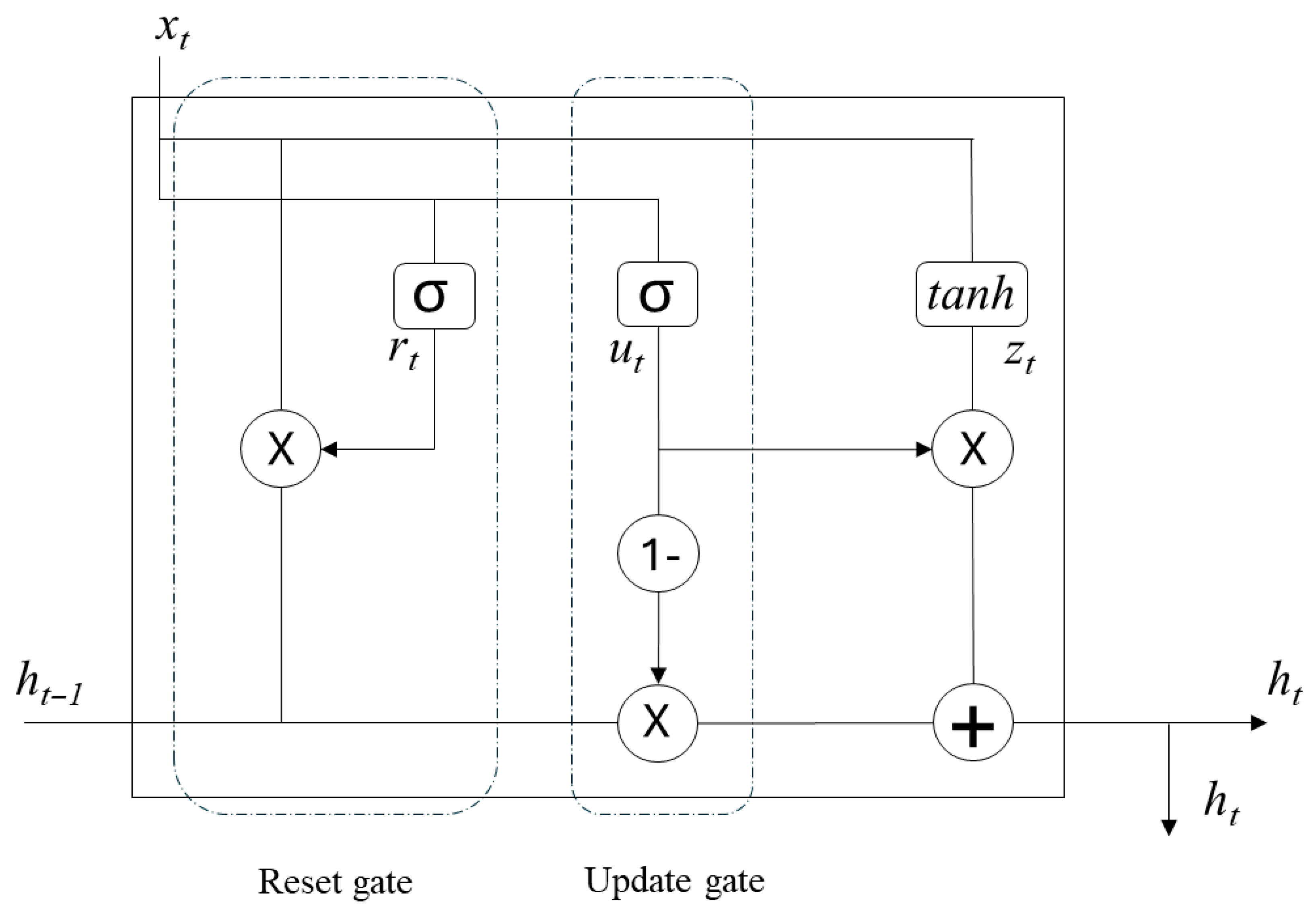
A GRU cell contains two key gates:
  • Update gate—Controls how much of the past information is retained versus updated with new input, effectively combining the roles of the input and forget gates in LSTM,
  • Reset gate—Determines how much of the previous state to discard when incorporating new input, enabling flexible integration of past and present information.
Figure 3 shows the GRU architecture. Compared to LSTMs, GRUs offer more compact architecture by reducing the number of gates and eliminating the separate cell state, relying solely on the hidden state for memory storage and propagation. This simplification leads to faster training and, in some cases, superior predictive performance, particularly when computational efficiency is a concern [69].
Owing to their effectiveness, GRUs have gained popularity across time series forecasting domains, including environmental applications, where they can capture nonlinear temporal dependencies between atmospheric precursors and pollutant concentrations with reduced computational overhead.
r t = σ   W x r x t + W h r h t 1 + b r
u t = σ   W x u x t + W h u h t 1 + b u
z t = t a n h W x z x t + W h z r t h t 1 + b z
c t = u t   h t 1 + 1 u t z t
where rt, ut refer to the states of reset gate and update gate, respectively, at time t, zt and ht represent candidate states and hidden states, respectively, Wxr, Whr, Wxz, Whz, Wxu, and Whu, are the trainable parameters, and the variables br, bu, and bz are the bias terms.

2.2.3. Hybrid Model

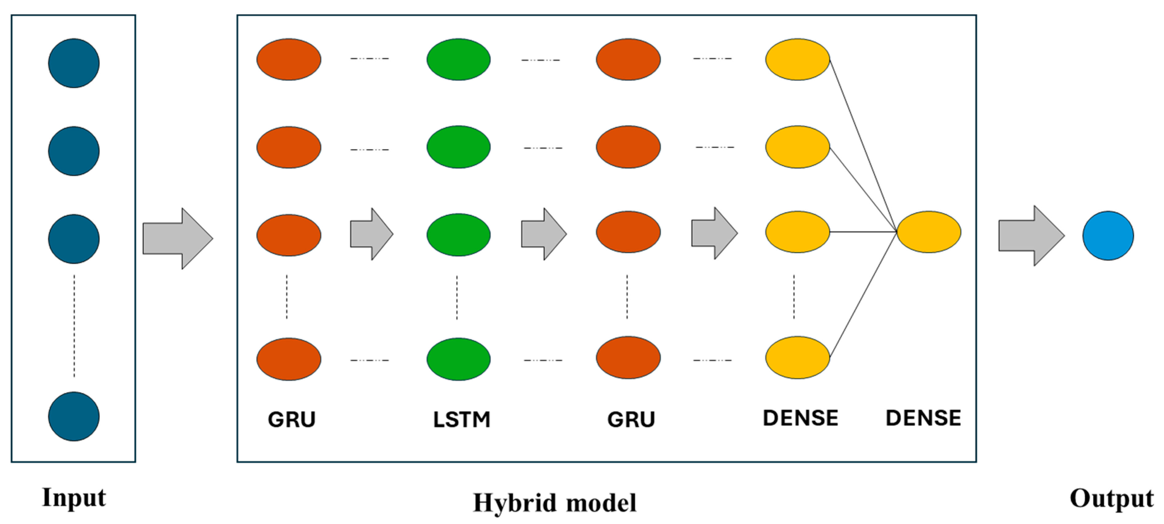
The proposed hybrid model integrates Gated Recurrent Unit (GRU) and Long Short-Term Memory (LSTM) layers in a sequential architecture designed to harness the complementary strengths of both RNN types for long-term ozone forecasting. This layered approach enhances the model’s capacity to capture both short-term fluctuations and long-range dependencies in complex environmental time series.
The architecture is constructed as follows:
  • First layer (GRU, 128 units): Processes the multivariate input sequence, capturing immediate temporal patterns, anomalies, and short-term dependencies, with fast convergence due to its simplified gating mechanism.
  • Second layer (LSTM, 128 units): Refines the intermediate representations by modeling deeper temporal structures, leveraging its input, forget, and output gates to selectively retain long-term information relevant to ozone formation dynamics.
  • Third layer (GRU, 128 units): Further abstracts the features, improving efficiency and stability by reinforcing learned temporal dependencies while minimizing computational overhead.
  • Fourth layer (Dense, 64 units): Acts as a fully connected layer that consolidates high-level representations from the recurrent layers into a compact feature space suitable for output prediction.
  • Final layer (Dense, 1 unit): Outputs the predicted 8 h average ozone concentration.
The data flow begins with the initial input being processed by the first GRU layer, subsequently directing its output into the LSTM layer for further processing. The output generated by the LSTM is then fed into a subsequent GRU layer. This architecture strategically combines the GRU’s ability to efficiently process recent trends and the LSTM’s superior capacity to retain long-term dependencies, enabling the model to capture multiscale temporal dynamics critical for accurate air quality forecasting. The structure of the proposed model is shown in Figure 4.
While training, the evaluation of the model’s performance is conducted through a cost function, which quantifies the difference between the predicted outputs and the actual values. Optimization is achieved by iteratively adjusting the weights to minimize the cost function, after which the optimized weights are stored for future forecasting tasks. These hybrid units combine the strengths of LSTM and GRUs to improve prediction accuracy and model robustness, making it well-suited for long-horizon forecasting in complex urban air quality systems.
Experimental Details and Model Performance Evaluations
In this study, we utilized Python 3.6 with Pandas, Numpy, Tensorflow, Scikit-learn, and Keras (accessed from https://www.python.org/ on 11 February 2025) to conduct data preprocessing and modeling.
The hybrid model was set up to use an 8 h sliding window to prepare the input data for time series forecasting of a sequential model. This technique will create a sequence of input–output pairs, which transform the time series data into a supervised learning problem. New input–output pairs are made as the window moves across the time series data. An example of this is shown below. For time series data: [ x 1 ,   x 2 ,   x 3 , x 4 , x 5 ,   ]
I n p u t   1 :   [ x 1 ,   x 2 ,   x 3 , x 4 , x 5 ,   x 6 ,   x 7 , x 8 ]   O u t p u t   1   [ x 9 ] I n p u t   2 :   [ x 2 ,   x 3 ,   x 4 , x 5 , x 6 ,   x 7 ,   x 8 , x 9 ]   O u t p u t   1   [ x 10 ] I n p u t   3 :   [   x 3 , x 4 , x 5 ,   x 6 ,   x 7 , x 8 ,   x 9 ,   x 10 ]   O u t p u t   1   [ x 11 ]
This process continues with a sliding window of one hour each time, creating a new input–output pair to train the LSTM-GRU hybrid model.
We trained the model to minimize mean squared error (MSE) and monitored mean absolute error (MAE) alongside RMSE and R2 for evaluation. Optimization used Adam (learning rate 2 × 10⁻³; β1 = 0.9, β2 = 0.999, ε = 10−7) with a mini-batch size of 64 and a maximum of 100 epochs. Hyperparameters were selected based on validation performance, and we employed Early Stopping [57] on validation loss (patience = 10 and restore_best_weights = True) to prevent overfitting and improve computational efficiency. Unless otherwise noted, loss refers to MSE in the hourly series. Random seeds were fixed for data windowing and weight initialization (Glorot uniform defaults) to ensure exact reproducibility. This is summarized in Table 2 below.
The model’s performance is assessed using a variety of statistical indices, such as the MSE, MAE, Root Mean Square Error (RMSE), Coefficient of Determination (R2), Mean Bias Error (MBE), mean absolute error (MAE), and Index of Agreement (IoA). These indices are defined as follows:
M S E = 1 n i = 1 n ( Y i Y ^ i ) 2
M A E = 1 n i = 1 n Y i Y i ^
R M S E = 1 n i = 1 n ( Y i Y ^ i ) 2
R 2 = 1 i = 1 n ( Y i Y ^ i ) 2 i = 1 n ( Y i Y i ¯ ) 2
M B E = 1 n i = 1 n Y i ^ Y i
I o A = 1 i = 1 n ( Y ^ i Y i ) 2 i = 1 n ( Y ^ Y i ¯ + Y i Y i ) 2
where n is the number of observed data; Y i is the observed value; Y ^ i is the predicted value; and Y i ¯ is the mean of observed values.
MSE is the most commonly used regression loss function. MSE averages the sample frame loss over the dataset. RMSE is the square root of MSE. It is more common than MSE since MSE can sometimes be too high to compare. The MAE measures the difference between two continuous variables, and the ideal model has an expected MAE value of zero. Both MAE and RMSE represent the amount of error between observed and predicted values, which are the most widely used performance metrics in many research areas, including ozone forecasting. Coefficient of Determination is a statistical measure that compares the fit of a regression line to actual data [70,71,72]. MBE indicates the systematic overestimation or underestimation of the model by providing positive and negative values, respectively. The IOA proposed by Willmott [73] is used to evaluate how well a predicted value fits an observed value, and its magnitude varies between 0 and 1. When two sequences are perfectly matched, IOA is equal to 1 [74].
We evaluate whether the proposed hybrid model achieves statistically significant accuracy gains over the RF baseline using the Diebold–Mariano (DM) [75] test for equal predictive accuracy. It is a robust statistical test that can be used to compare the accuracy of forecasting models without assuming a specific distribution of forecasting errors [44]. For model m, define the one-step error. Let e t ( m ) = y t   y ^ t m . For squared-error loss (analogously for absolute error), the loss differential is
d t = e t ( H y b r i d ) 2 e t ( R F ) 2
We test H0: E[dt] = 0 using the classical DM statistics:
D M = d ¯ V a r ^ ( d ¯ ) ,   w i t h   V a r ^ d ¯ =   s d 2 T  
where d ¯ is the sample mean of d t t = 1 T , s d 2 is its sample variance, and T is the evaluation length. This corresponds to the lag-0 (no serial-correlation adjustment) version of the test, appropriate when one-step-ahead loss differentials are approximately uncorrelated. We report two specifications of the loss function—MSE and MAE—to ensure findings are not an artifact of a single loss choice. Here, we compared the proposed hybrid model with the Random Forest (RF) model. Alongside hypothesis tests, we report effect sizes: the difference in RMSE, Δ RMSE = RMSE Hybrid − RMSE RF, the percent RMSE reduction, and the explained-variance gain Δ R2 = R2Hybrid − R2RF [76].
The selection of units and layers in the model structures is summarized in Table 1. The learning capacity of a neural network is directly represented by the number of hidden units and layers, which represent the network’s width and depth, respectively.

2.3. Results and Discussion

In this analysis, we first examined the temporal variability of all predictor variables to understand seasonal and diurnal patterns. Next, we assessed the feature importance of each independent variable relative to ozone concentrations to identify the most relevant inputs for modeling. Finally, we developed the hybrid GRU-LSTM model and evaluated its performance using multiple statistical metrics to assess its ability to predict ground-level ozone concentrations over multi-year periods.

2.3.1. Overview of Parameters in the Fort Worth Northwest Region

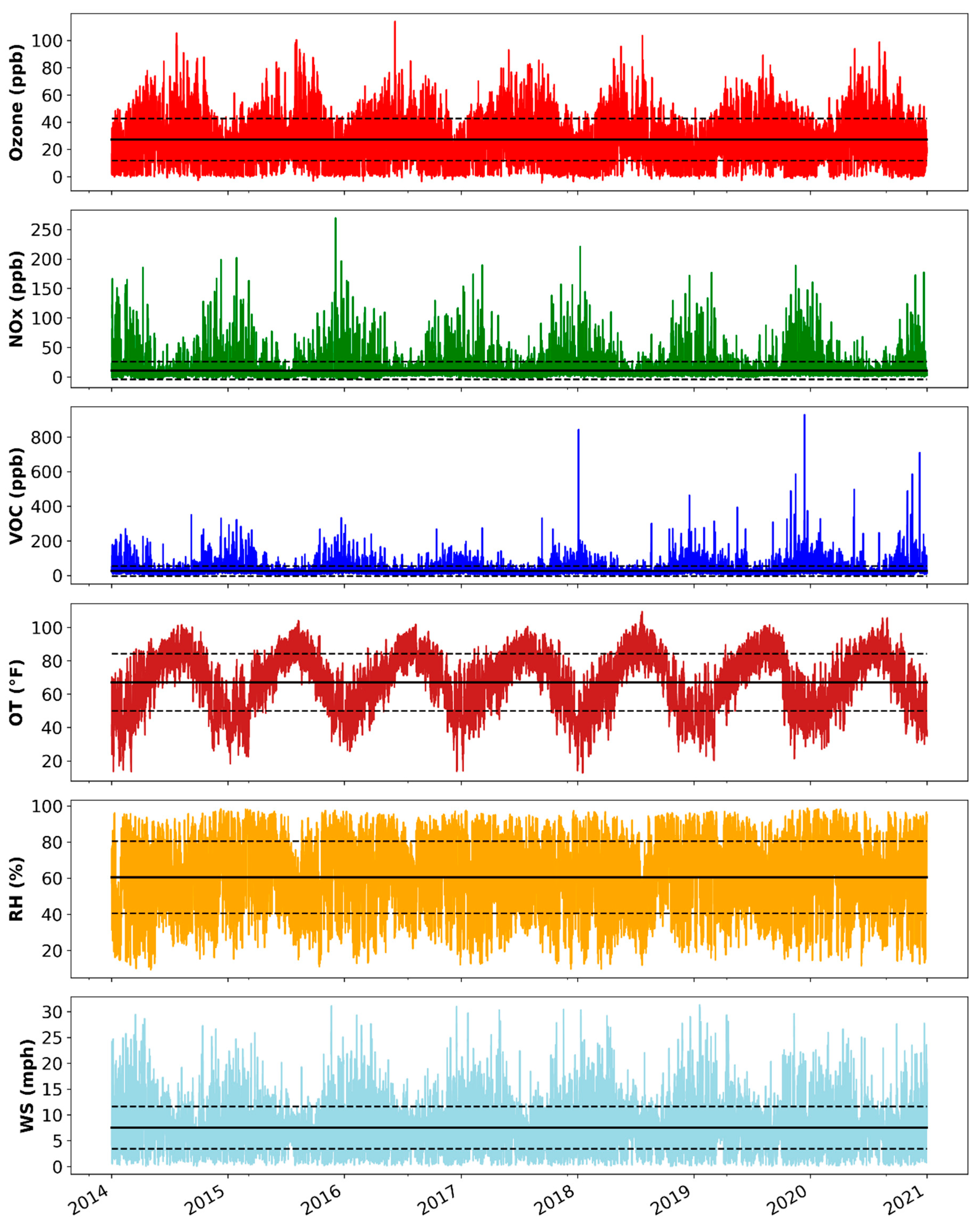
Figure 5 presents the temporal variations in air pollutant concentrations and meteorological variables at CAMS 013 from January 2014 to December 2020, while Supplementary Figure S1 displays additional meteorological trends. To improve interpretability, total VOC concentrations are shown in aggregate, though all 22 individual VOC species were included in the modeling framework. Over the study period, average concentrations were as follows: ozone, 27.14 ± 15.48 ppb; NOx, 10.83 ± 15.02 ppb; and VOCs, 25.66 ± 28.97 ppb. Despite relatively low standard deviations, NOx and VOCs exhibited substantial fluctuations, driven by frequent low baseline values punctuated by episodic high-concentration events.
As shown in Table 1, the skewness value provides insight into the distribution of the pollutants. Ozone with a skewness of 0.53 suggests that the distribution of slightly skewed to the right. This indicates that ozone values are close to average, with a small number of higher concentrations pulling the distribution to the right. A skewness value of 4.02 for NOx indicates a highly right-skewed distribution, suggesting many lower values, but with a significant tail of higher concentrations. It implies that extreme NOx events occur less frequently but are much higher than the typical values. A skewness value of 5.64 for VOC indicates an even more pronounced right skewness. This suggests that most VOC concentrations are low, but there are some very high spikes in VOC levels. Seasonal trends were consistent across years. Ozone peaked during midyear (summer) and aligned with elevated outdoor temperature (OT), solar radiation (SR), and dew point (DP), reflecting enhanced photochemical production under warm, sunlit conditions. Conversely, NOx, VOCs, and wind speed (WS) were elevated during cooler months, while relative humidity (RH) followed a stable seasonal cycle.
The study site, located in the Barnett Shale region, has been impacted by substantial oil and gas activities, particularly in post-2019 when hydrocarbon production surged [55]. Ozone design values at this site have exceeded the National Ambient Air Quality Standards (NAAQS) over the past two decades. Although design values showed a declining trend until 2019, they began rising again from 2020 onward [56], consistently remaining above regulatory thresholds throughout the study period.
The monthly average concentrations of air pollutants in CAMS 013 showed pronounced seasonal variability. As depicted in Figure 6a, ozone levels peaked between April and October, driven by intensified photochemical activity during warmer months. In contrast, NOx and VOC concentrations were elevated from October to March, likely reflecting reduced photochemical loss and less favorable dispersion conditions during winter [77,78].
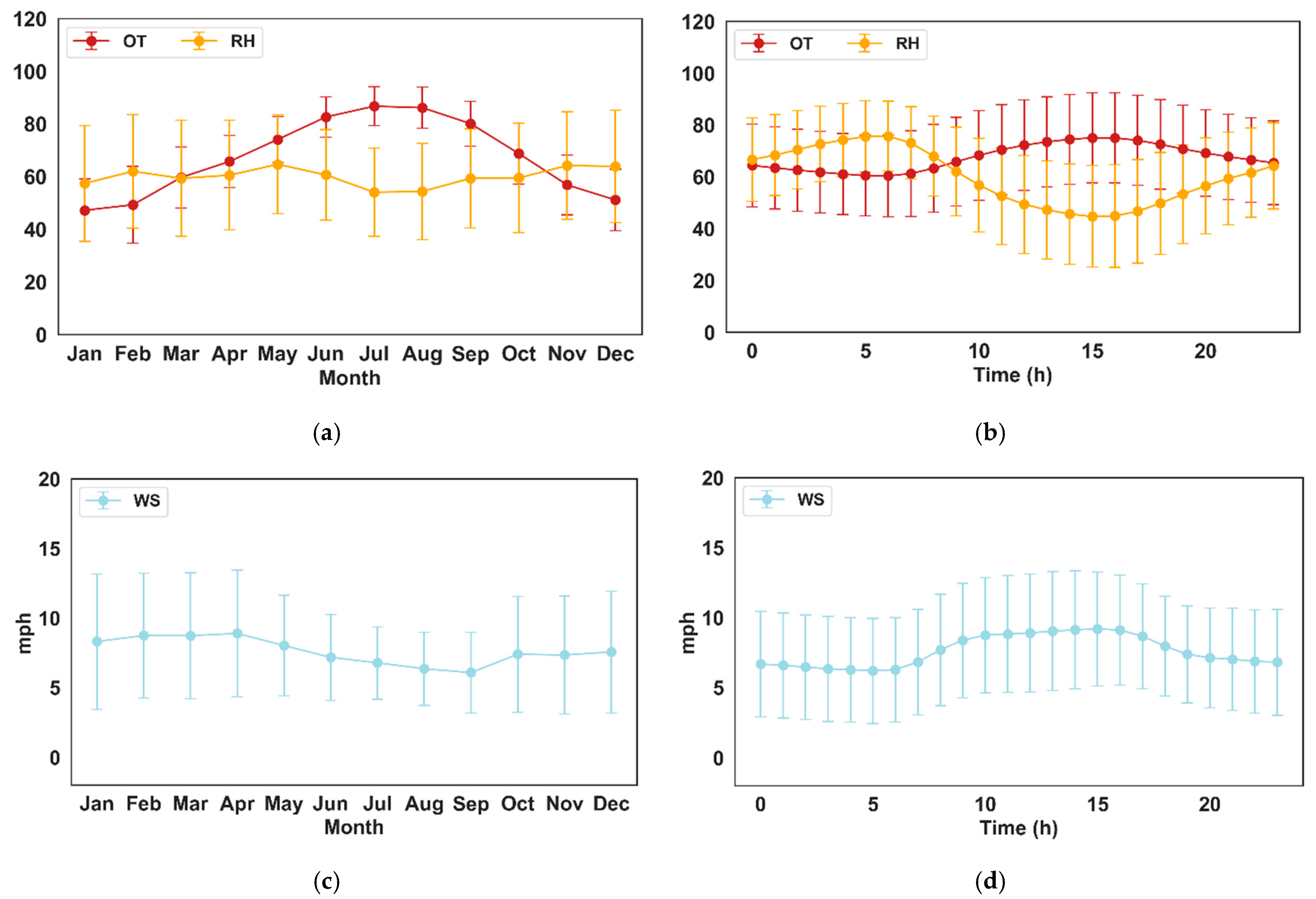
Daily pollutant patterns mirrored these seasonal effects (Figure 6b). During summer, outdoor temperature (OT) and dew point (DP) increased (Figure 7a), supporting photochemical ozone formation. Wind speed (WS) declined from June to September, with midday (10:00–16:00) increases (Figure 7c,d). Relative humidity (RH) was higher during nighttime and early morning (17:00–10:00) and lower in the afternoon (11:00–18:00). Peak wind gust (PWG), WS, and wind direction (WD) exhibited slight midday increases, while DP and solar radiation (SR) showed minimal diurnal variation.
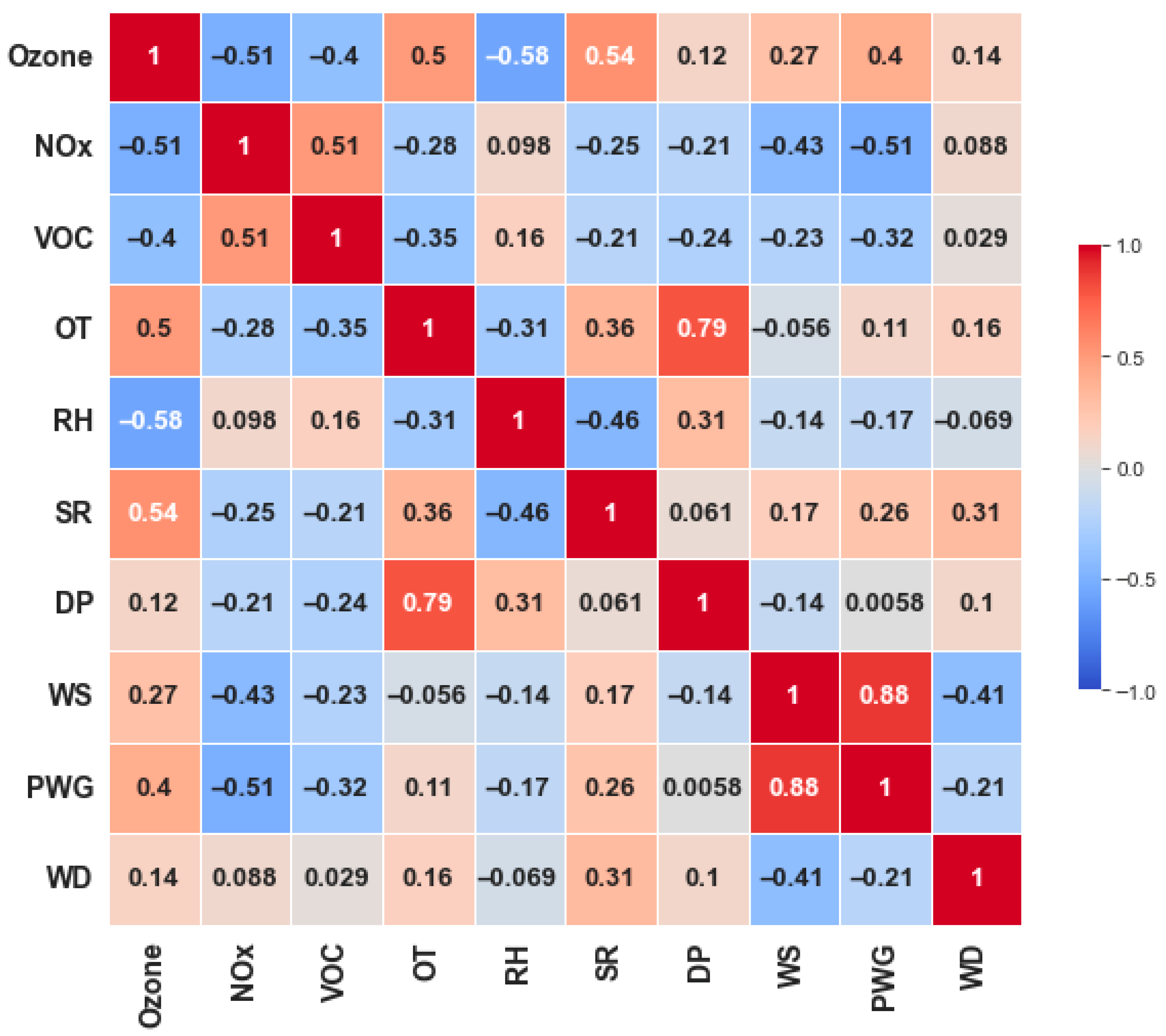
We used a correlation matrix to quantify inter-variable relationships. Figure 8 shows the heatmap for meteorological parameters, NOx, ozone, and the sum of all the VOCs. Figure S2 shows the heatmap for all the parameters, with individual VOCs, used in the study. Notable findings included the following: strong positive correlation between WS and PWG (r = 0.88), indicating faster winds produce stronger gusts; positive correlations between ozone and OT (r = 0.50), SR (r = 0.54), and PWG (r = 0.40), consistent with enhanced photochemical production under warm, sunlit, turbulent conditions; weaker positive correlations between ozone and WS (r = 0.27), WD (r = 0.14), and DP (r = 0.12); and negative correlations between ozone and NOx (r = −0.51), VOC (r = −0.40), and RH (r = −0.58), reflecting titration effects and inverse humidity–ozone dynamics [79,80].
Although some variables showed weak or negative individual correlations with ozone, their combined interactions are essential for predictive modeling. Together, the observed diurnal, seasonal, and inter-variable relationships highlight the complex, coupled dynamics governing ozone variability—supporting their integration into the hybrid model to improve forecasting performance.

2.3.2. Feature Importance Evaluation

Before model training, we analyzed the relationships between independent variables (pollutants and meteorological parameters) and ozone concentrations to identify the most relevant predictors. Feature selection was used to improve model interpretability and computational efficiency. We employed SHAP for feature selection [81,82,83,84]. SHAP, grounded in cooperative game theory, quantifies each feature’s contribution to the model’s output. Specifically, we applied Random Forest (RF) as the base supervised learning model for SHAP analysis, leveraging its ability to handle complex, high-dimensional data and minimize overfitting through ensemble bagging [85,86,87]. RF calculates feature importance by measuring reductions in node impurity across decision splits.
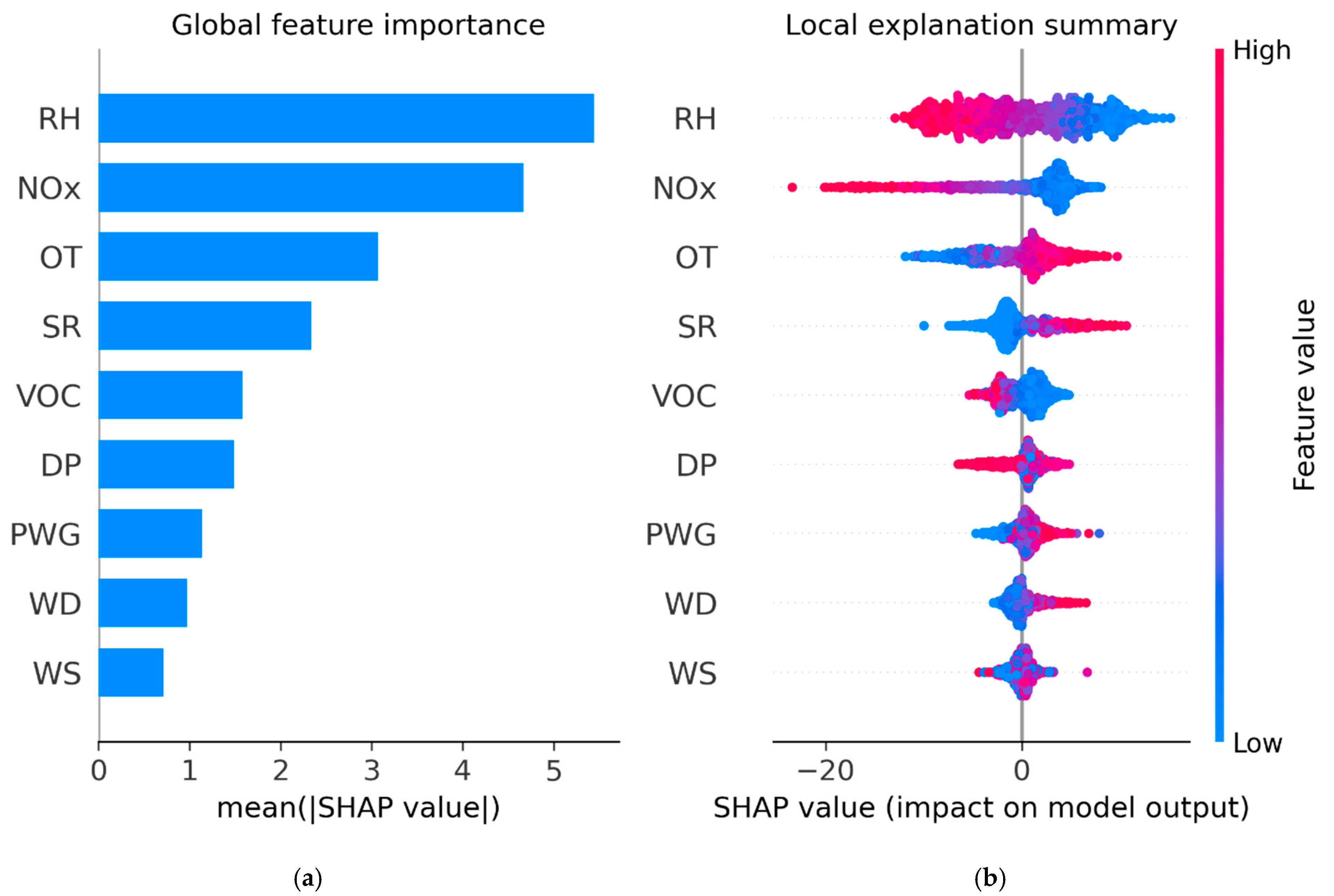
Figure 9a presents the SHAP summary plot, showing the mean absolute impact of each feature on ozone predictions, while Figure 9b illustrates the directional influence of each feature value. Positive SHAP values indicate a feature’s contribution to increasing ozone forecasts, whereas negative values indicate contributions to decreasing them.
Results revealed that RH was the most influential feature, with higher RH linked to lower predicted ozone and lower RH linked to higher ozone—consistent with its negative correlation in the matrix (Figure 8). Similar negative influences were observed for NOx, VOC, and DP. Conversely, OT and SR showed strong positive associations, with higher values driving elevated ozone levels. These insights align with known photochemical dynamics and reinforce the mechanistic consistency of the model.

2.3.3. Prediction Using a Hybrid Model

The first step in developing the ozone forecasting framework was to determine the feasible prediction horizon. While prior studies have shown that longer lead times typically reduce forecast accuracy [45], our study extended beyond short-term horizons by forecasting hourly ozone concentrations over a full annual cycle. Specifically, the model was trained on data from 2014 to 2020 and tested on data from 2021 to 2023. Data from early 2024 were excluded due to incomplete records (available only until 31 March).
As described in Section “Experimental Details and Model Performance Evaluations”, we employed an 8 h rolling window to construct input sequences. This window length was selected to capture temporal dependencies relevant to ozone dynamics and is consistent with health-relevant exposure periods. Studies have shown that 8 h (or longer) ozone exposures typically capture 75–90% of the daily maximum 1 h ozone values and are more reliable indicators of photochemical pollution episodes than 1 h maxima [86]. The choice of the 8 h averaging period also aligns with regulatory standards, balancing community exposure durations, health effect relationships, and monitoring practices [88,89].
To optimize the model’s hyperparameters, we employed Keras Tuner, an automated optimization tool that explores combinations of parameters (e.g., learning rate, batch size, dropout) using cross-validation to identify settings that maximize predictive performance. Additionally, select hyperparameters were fine-tuned manually to further improve accuracy and training efficiency.
We incorporated Early Stopping regularization during model training to prevent overfitting by halting the process when validation loss plateaued. The final model achieved optimal performance at epoch 39, yielding low training and validation losses (training loss = 0.0018, validation loss = 0.0019) and minimal mean absolute error (training MAE = 0.0315, validation MAE = 0.0328), indicating excellent fit and generalization across the datasets. Figure 10 presents the epoch-wise training curves for loss and MAE.
Figure S3 shows the loss and MAE for training and validation throughout the different epochs. Both training and validation metrics rapidly decreased during the first ~10 epochs and then stabilized at low values (training loss ≈ 0.0018, training MAE ≈ 0.0315; validation loss ≈ 0.0019, validation MAE ≈ 0.0328). The similarity of the training and validation curves reflects good generalization with no indication of overfitting. Minor fluctuations in validation MAE were expected because of the variability in the high ozone days; nonetheless, these fluctuations were controlled throughout the epochs. In conclusion, the model reached a stable regimen with a good fit, achieving confidence in predicting unseen data.
Model performance was evaluated using standard time series forecasting metrics, including MSE, RMSE, MAE, R2, MBE, and IoA, widely applied in air pollution studies [29,30,90,91,92]. Notably, when benchmarked against alternative models—Random Forest (RF), standalone LSTM, the hybrid model consistently outperformed the baseline models (Figures S4 and S5).
Forecasting Ozone in Fort Worth Northwest
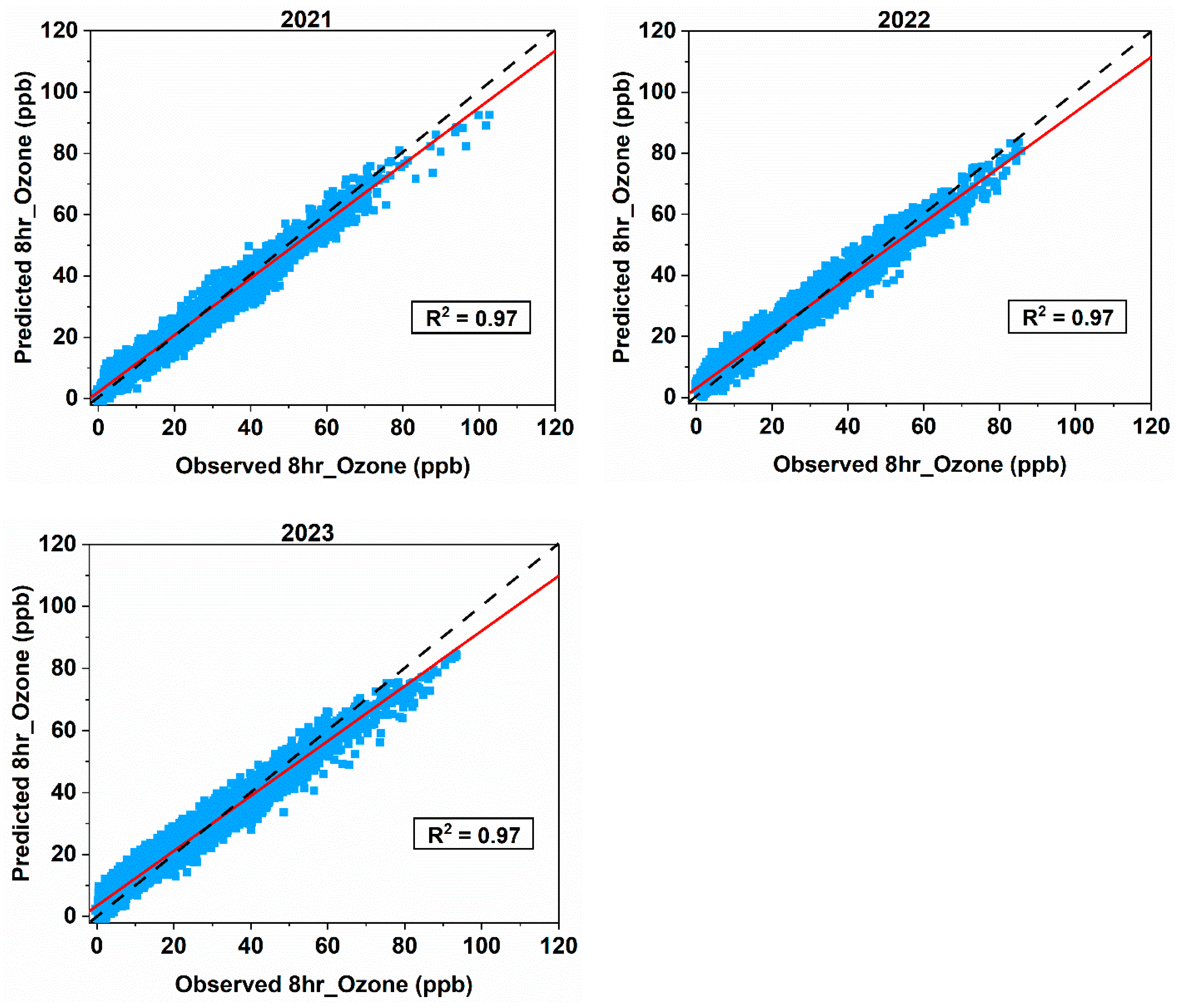
The hybrid model was trained to predict hourly ozone concentrations for the years 2021–2023, from which 8 h rolling averages were subsequently computed to align with regulatory ozone standards and to evaluate model performance in terms of metrics relevant to air quality management. The correlation between predicted and observed ozone levels was analyzed for each year. As shown in Figure 10, the predicted values align closely with observations, with R2 values of 0.97 for all years, indicating that the model explains 97% of the variance in ozone concentrations—an excellent fit across multiple years. Figure S6 shows the correlation plot between observed and predicted ozone concentrations in CAMS013.
Figure S7 presents the complete time series plots of observed and predicted ozone concentrations for all years in CAMS013. Table 3 summarizes the annual model evaluation metrics. Key findings include, during 2021, MSE = 24.81, RMSE = 4.98, reflecting low prediction error and strong agreement; during 2022–2023, slight increases in MSE and RMSE suggest marginally reduced accuracy relative to 2021, although performance remained robust overall.
The consistently high R2 values highlight the model’s strong predictive capability. Negative MBE values for all years indicate a slight underprediction bias, most pronounced in 2023 (MBE = −0.59) compared to 2021 (−0.48) and 2022 (−0.37). Importantly, the IoA exceeded 0.96 across all years, confirming excellent agreement between predicted and observed ozone levels.
These results demonstrate that the hybrid GRU-LSTM model reliably captures both temporal trends and the magnitude of ozone concentrations, providing a robust tool for long-term forecasting in complex urban air quality regimes.
On CAMS013, for the year 2021, the proposed hybrid model outperforms the RF baseline across all metrics for hourly ozone (Hybrid: RMSE = 4.98, MAE = 3.6, R2 = 0.91; RF: RMSE = 7.57, MAE = 5.95, R2 = 0.79), yielding an absolute improvement of ΔRMSE = −2.59 (a 34.12% RMSE reduction) and an explained-variance gain of ΔR2 = +0.12 (12%).
Classical Diebold–Mariano tests reject equal predictive accuracy for both scoring rules, MSE loss t = −9.23, p = 2.69 × 10⁻²⁰; MAE loss t = −10.62, and p = 2.41 × 10⁻²⁶, corroborating that the hybrid model’s improvements are statistically robust on CAMS013 for the year 2021.
Forecasting High-Ozone Events in Fort Worth Northwest
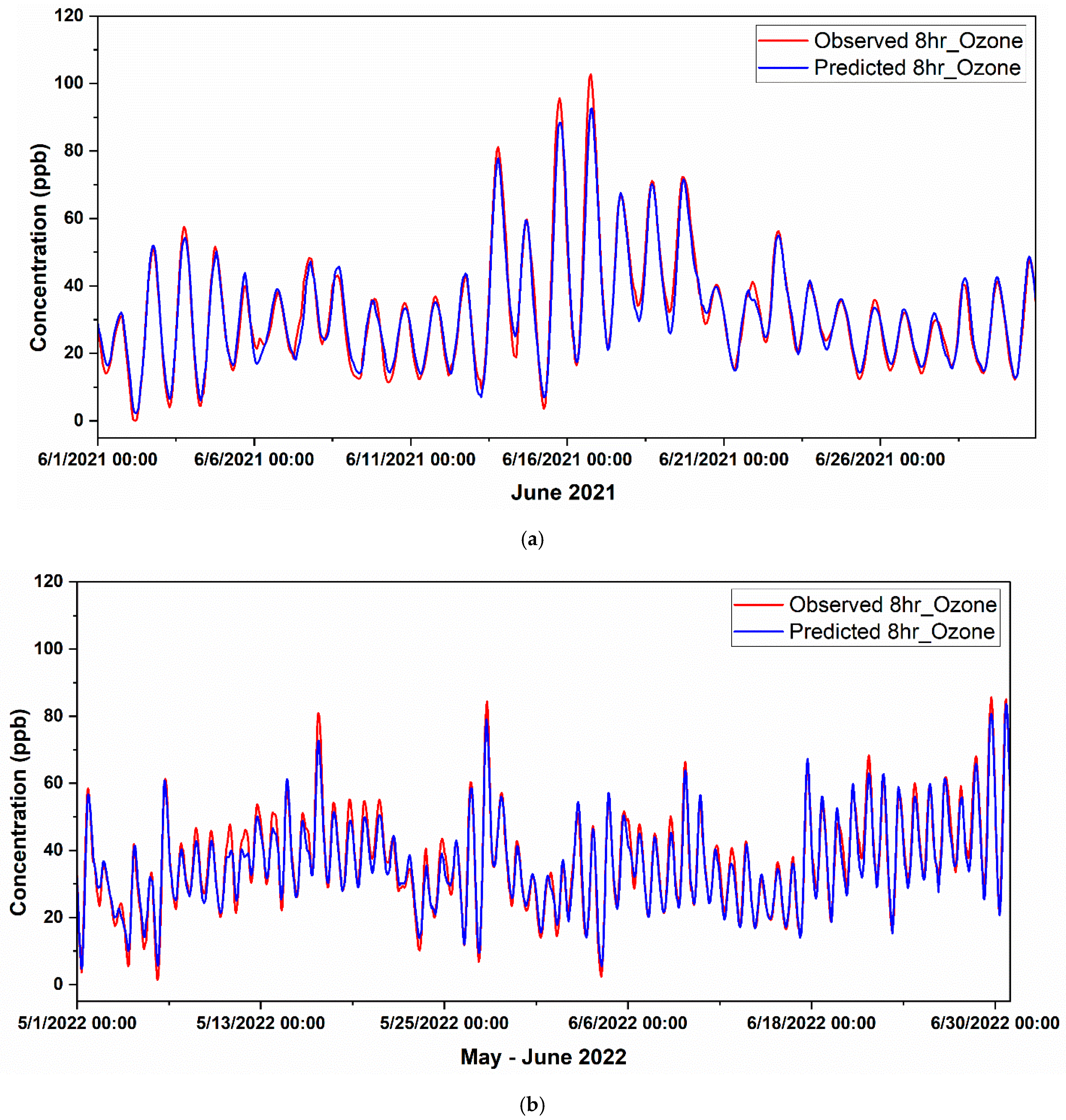
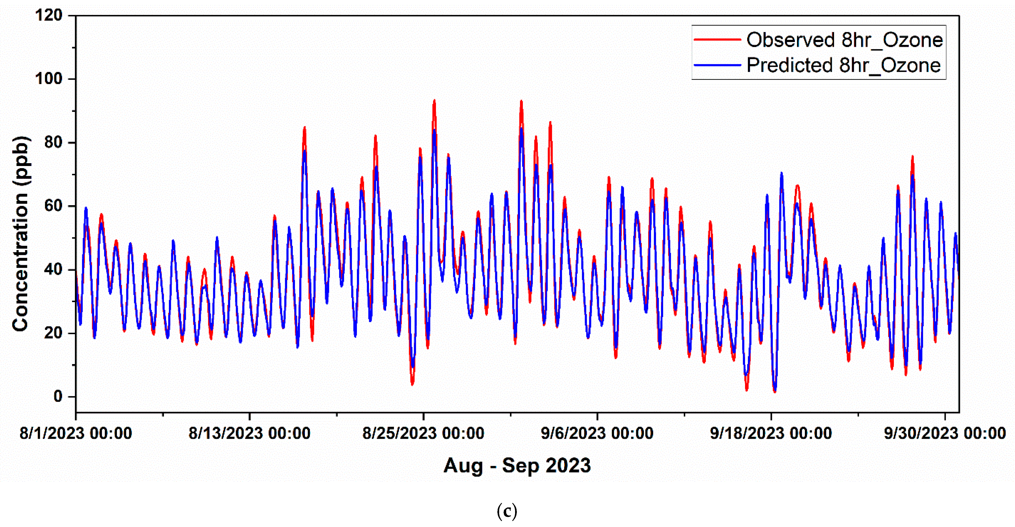
To further evaluate model performance during critical pollution events, we analyzed high-ozone episodes from 2021 to 2023, defined as days when the 8 h average ozone concentration exceeded 70 ppb. Peak hours were identified across multiple summer months (June–September), prompting a focus on the months with the highest frequency of exceedances.
Figure 11 highlights these high ozone months for each year. During 2021, June recorded six high-ozone days, and the model achieved an R2 of 0.98, indicating excellent agreement between observed and predicted concentrations (Figure 11a). The model closely tracked both the diurnal cycles and the peak episodes, with only minor underestimation of the sharpest exceedances. This high level of accuracy highlights the model’s ability to reproduce conditions well-represented in the training dataset.
In 2022, the peak ozone activity shifted earlier in the season, with three exceedance days in May and five in June. The model maintained strong performance with an R2 of 0.96 for this combined period (Figure 11b). Although predictions slightly underestimated certain peak values, the temporal alignment with observed high-ozone episodes remained robust. The slightly reduced performance relative to 2021 may be attributed to the unusually elevated ozone concentrations during 2022.
By 2023, the highest ozone activity occurred later in the season, concentrated in August and September, with seven and eight high-ozone days, respectively. The model again achieved strong predictive skill, with an R2 of 0.97 (Figure 11c), closely replicating the observed diurnal and episodic patterns. As with prior years, some peak magnitudes were modestly underpredicted, but the model consistently reproduced the variability of exceedance events.
Overall, while the model slightly underpredicted some of the peaks and troughs during high ozone days, it consistently captured the overall temporal patterns and magnitudes. Supplementary Figure S8a–d presents additional results for low-ozone day predictions at CAMS 013. These findings demonstrate the hybrid model’s capacity to maintain predictive accuracy not only under average conditions but also during extreme air pollution episodes.
Forecasting Ozone in Dallas Hinton
The developed forecasting model using the CAMS 013 (Fort Worth Northwest) data from 2014 to 2020 was used to predict the ozone concentrations at the CAMS 0161 (Dallas Hinton) location. We predicted the ozone values from 2015 through 2019 for CAMS 0161. Figure 12 shows the correlation plot between the observed and predicted 8 h ozone concentrations for each year, showing that predictions are consistent with the observations in this region. The R2 by the years is as follows: 2015 (R2 = 0.95), 2016 (R2 = 0.95), 2017 (R2 = 0.94), 2018 (R2 = 0.95), and 2019 (R2 = 0.94).
The forecasting results indicate that the hybrid model performs efficiently in predicting the ozone concentrations at CAMS 0161 for each year, with R2 = 0.95 during the years 2015, 2016, and 2018 and R2 = 0.94 during the years 2017 and 2019 showing that the model trained with the CAMS 013 data was able to explain the CAMS 0161 ozone concentrations efficiently. Figure S9 shows the complete time series plot with observed and predicted 8 h ozone concentrations for all the years. However, the overall performance of the model was slightly lower than that observed at CAMS 013. Table 4 shows the performance evaluation parameters of this model. The model performance shows a slight deterioration for CMAS 0161. The MSE and RMSE values exhibited a slight increase compared to the prediction of CAMS 013.
The model performance for the years ranging from 2015 to 2019 gave quite high predictive accuracy and agreement with observed data, as shown by the quite stable IoA values ranging between 0.95 and 0.97. The best performance of the model in 2015 attained a minimum MSE of 30.37, which means a very small bias and, therefore, very good precision. It has small increases in MSE and bias from 2016 to 2018; however, for the same period, IoA is very strong at 0.96, indicating stable performance. In addition, 2019 shows a very high decline, with the highest MSE of 33.59, RMSE of 5.80, and MBE of −1.07, showing that the prediction error with bias is increasing. In general, the model is performing well; however, the trend indicates that there has been a modest decline in accuracy over time.
The model’s ability to reproduce both high- and low-ozone conditions across multiple years is further illustrated in Figure S8a–d, showing detailed low-ozone day predictions. Overall, these results confirm the hybrid model’s strong generalization ability across sites and its capability to capture seasonal ozone dynamics, although slight reductions in performance were observed during years with more complex or extreme pollution patterns.
Forecasting High-Ozone Events in Dallas Hinton
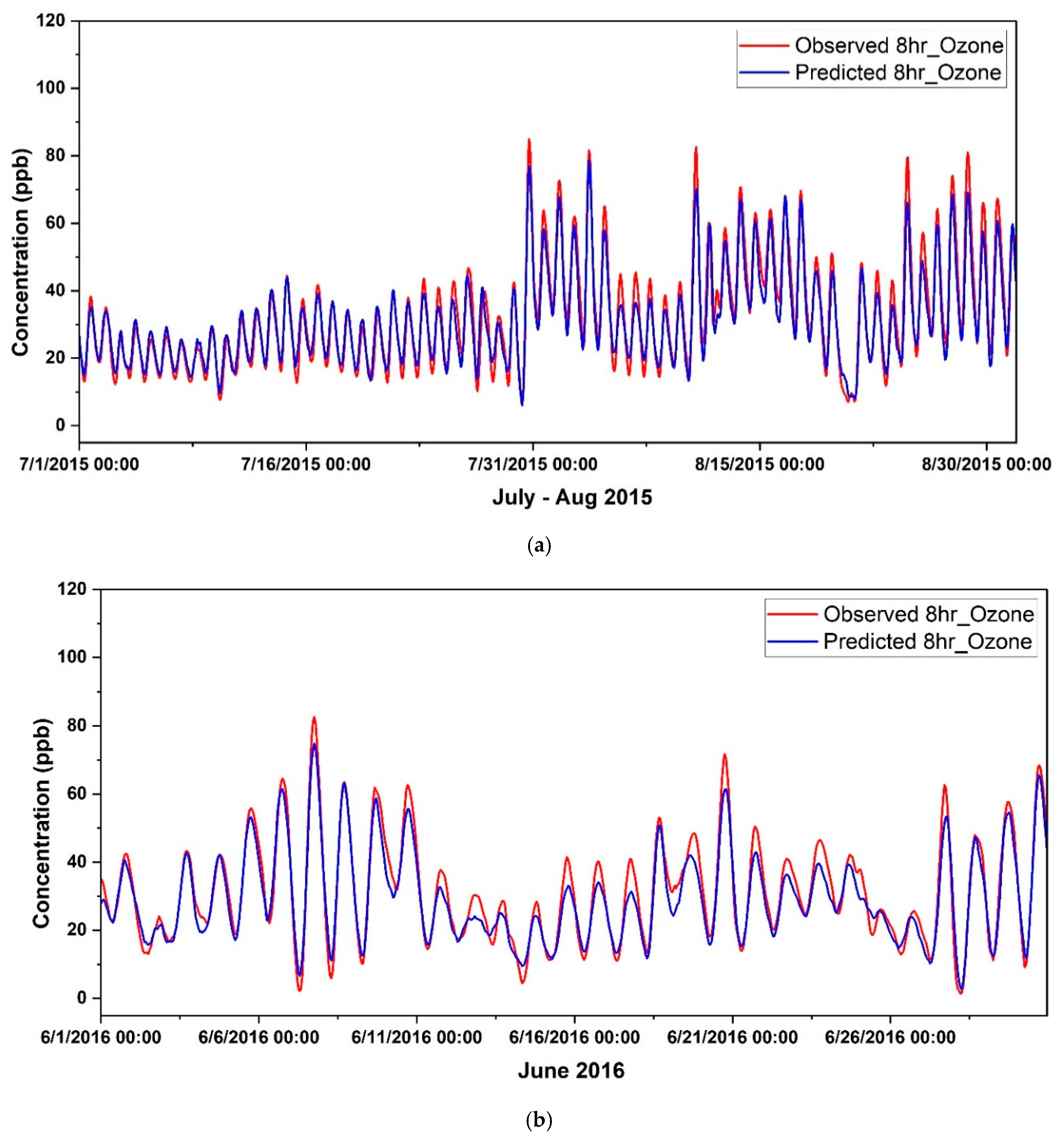
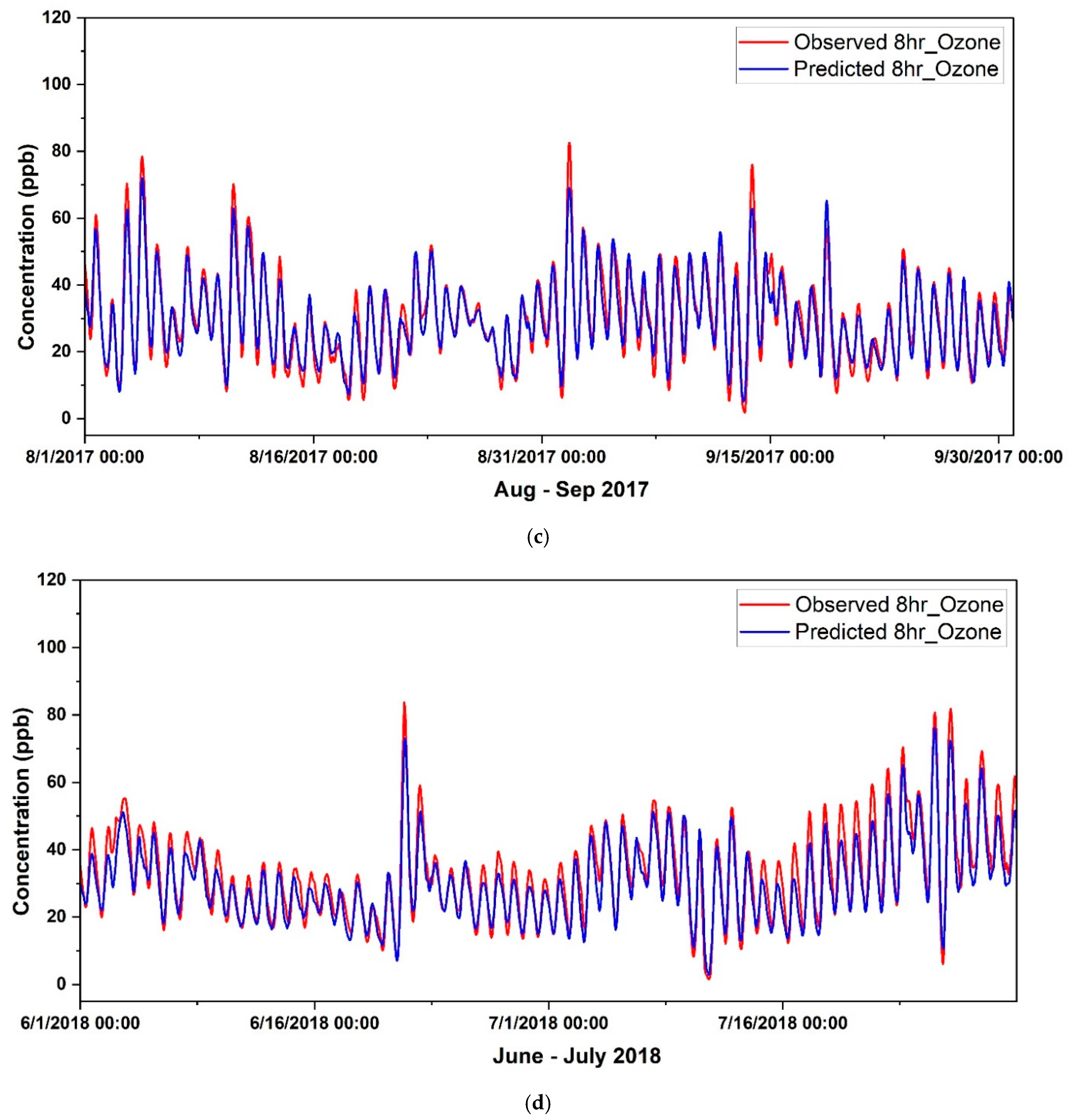
We observed at CAMS 013 multiple peak hours clustered during the summer months, particularly June to September. We focused on the hours and months with the highest number of exceedance days. Figure 13 highlights the key high ozone periods across the years: In 2015, the July–August period was marked by clustered exceedances, with a total of 37 h above the 70 ppb threshold. While July also included several low-ozone days, the model reproduced these transitions with high reliability, reflected in an overall R2 of 0.96 for the entire period. However, when evaluated solely on exceedance hours, the R2 dropped to 0.45, underscoring that while background and moderate ozone levels are modeled with high precision, the most extreme peaks remain more difficult to capture. This tendency is also visible in Figure 13a, where the predicted peaks slightly underestimate observed values, indicating a systematic underprediction bias at higher concentrations.
In 2016, June emerged as the most critical month for high ozone, and the model again achieved excellent agreement with observations (R2 = 0.96). The line plot shows that both the amplitude and timing of high-ozone peaks are well-reproduced, including several episodes exceeding 70 ppb. This suggests that the 2016 meteorological and precursor conditions were well-aligned with the model’s training data, allowing it to generalize effectively.
During 2017 and 2018, high-ozone episodes were concentrated in August–September (2017) and June–July (2018). The model maintained strong performance with R2 values around 0.94, slightly lower than in 2015–2016 but still robust. The time series plots confirm that most exceedance peaks are well-captured, although occasional underestimation of the highest spikes is evident, particularly in 2017. In 2018, the diurnal cycle of ozone was predicted with notable accuracy, with good alignment in both peak hours and background values. This reinforces the model’s strength in capturing short-term temporal dynamics across multiple summer seasons.
The model showed strong performance in capturing daily and seasonal ozone variability across years, with R2 values above 0.94 for full-month predictions. Overall, the framework is robust across different meteorological conditions but tends to underpredict peak concentrations, suggesting the need for enhanced features or bias correction to improve high-ozone forecasting.
Although the hybrid GRU–LSTM framework exhibits consistently strong skill across years and sites, several methodological considerations merit note. First, the capacity of deep sequence models introduces a risk of overfitting in the presence of pronounced diurnal and seasonal structure; we addressed this through nested validation, Early Stopping, dropout, and L2 regularization, and we report epoch-wise learning behavior to document small train–validation gaps. Second, model performance shows some sensitivity to hyperparameter choices; repeated-seed training and constrained tuning budgets indicate modest variance, but further robustness could be obtained via lightweight ensembling. Third, restricting inputs to 1 h lags emphasizes near-term photochemical and titration dynamics but may under-represent synoptic evolution; the lag–window sensitivity analysis indicates incremental gains up to 6–12 h with diminishing returns beyond one diurnal cycle. Finally, a mild underprediction of extreme peaks is observed during certain high-ozone episodes; quantile-oriented objectives or post hoc bias correction could improve tail fidelity without compromising baseline accuracy.

3. Conclusions

This study developed a novel hybrid recurrent neural network (RNN) model that integrates Gated Recurrent Unit (GRU) and Long Short-Term Memory (LSTM) layers to forecast ground-level ozone concentrations across multiple years and locations. The model leveraged ozone precursor concentrations (NOx, 22 VOC species), seven meteorological variables, and one-hour lagged inputs to effectively capture both short- and long-term temporal dependencies. An 8 h sliding window framework was applied to align with the photochemical timescales relevant to ozone formation and regulatory standards. The key findings and contributions are summarized below:
  • Trained on CAMS 013 data (2014–2020) and tested on 2021–2023 data, the model achieved an R2 of 0.97, accurately identifying high-ozone episodes with stable performance across all years.
  • When applied to CAMS 0161 (2015–2019), the model demonstrated strong generalization capability, achieving R2 values of 0.94–0.95. Although slight underprediction biases were observed (MBE: −0.13 to −1.07), the overall agreement with observations remained high (IoA > 0.95).
  • The model maintained high predictive accuracy for high-ozone days, with R2 values ranging from 0.96 to 0.98 at CAMS 013 and 0.94 to 0.96 at CAMS 0161, effectively capturing interannual and seasonal ozone dynamics. However, it slightly underpredicted extreme peaks, indicating the potential for further refinement.
The framework reliably captures temporal patterns but underpredicts extreme peaks, underscoring its strength for region-specific forecasting and the need for refinement to improve the prediction of extreme concentrations. Importantly, the proposed hybrid architecture outperformed traditional models (e.g., standalone LSTM, GRU, and RF), showcasing its capacity to capture the nonlinear, time-dependent dynamics of ozone formation under varying meteorological and emission conditions. This work offers a robust, interpretable, and transferable framework for long-term ozone forecasting, with significant potential to support regional air quality management and regulatory decision-making.

Supplementary Materials

The following supporting information can be downloaded at: https://www.mdpi.com/article/10.3390/app152211923/s1, Figure S1: Time series of all the parameters for SR, DP, WD, and PWG for complete study period in CAMS013; Figure S2: Heatmap of correlation matrix between all the variables in CAMS013 for the study period; Figure S3: Model training history; Figure S4: Model prediction of RF for 2020 (scaled data); Figure S5: Model prediction of LSTM for 2020; Figure S6: Correlation between observed and predicted ozone for CAMS013 with best fit line; R2 value and Pearson correlation value, r; Figure S7: Time series forecast for 8 h ozone concentrations during complete years in (a) 2021, (b) 2022, and (c) 2023 for CAMS013; Figure S8: Time series forecast for 8 h low ozone concentrations during (a) 2021, (b) 2022, and (c) and (d) 2023 for CAMS013; Figure S9: Correlation between observed and predicted 8 h high ozone for CAMS 013 with best fit line; R2 value for years from 2021 to 2023.

Author Contributions

Conceptualization, K.J.; Methodology, J.K.; Software, A.A.M.; Validation, A.A.M.; Formal analysis, J.K.; Investigation, J.K.; Resources, K.J.; Data curation, A.A.M.; Writing—original draft, J.K.; Writing—review & editing, K.J.; Visualization, J.K.; Supervision, K.J.; Project administration, K.J. All authors have read and agreed to the published version of the manuscript.

Funding

This research received no external funding.

Institutional Review Board Statement

Not applicable.

Informed Consent Statement

Not applicable.

Data Availability Statement

The original data presented in the study are openly available at https://github.com/jithinkpoyil/Hybrid-model-for-ozone-forecasting (accessed on 2 November 2025). The raw data supporting the conclusions of this article will be made available by the authors on request.

Acknowledgments

The authors would like to acknowledge the Texas Commission on Environmental Quality (TCEQ) for providing ambient air quality monitoring data through their publicly accessible TAMIS online data portal (http://www17.tceq.texas.gov/tamis/index.cfm) (accessed on 10 January 2025). The findings and opinions expressed in this study are solely those of the authors. They do not represent the views of their employer nor of any of the agencies mentioned above that were instrumental in providing the relevant data. The authors used OpenAI tools (ChatGPT-5) (https://openai.com/index/chatgpt/, accessed on 17 September 2025) to assist with linguistic improvements. No generative content or scientific interpretations were produced by the tool.

Conflicts of Interest

The authors declare no conflicts of interest.

References

  1. Chen, T.M.; Kuschner, W.G.; Gokhale, J.; Shofer, S. Outdoor Air Pollution: Ozone Health Effects. Am. J. Med. Sci. 2007, 333, 244–248. [Google Scholar] [CrossRef]
  2. WHO. Review of Evidence on Health Aspects of Air Pollution–RE-VIHAAP Project: Technical Report. Tech. Doc. WHO/EURO:2013-4101-43860-61757. 2013. 309p. Available online: https://apps.who.int/iris/bitstream/handle/10665/341712/WHO-EURO-2013-4101-43860-61757-eng.pdf?sequence=1&isAllowed=y (accessed on 3 August 2025).
  3. Bell, M.L.; Zanobetti, A.; Dominici, F. Who is more affected by ozone pollution? A systematic review and metaanalysis. Am. J. Epidemiol. 2014, 180, 15–28. [Google Scholar] [CrossRef]
  4. Mills, G.; Pleijel, H.; Malley, C.S.; Sinha, B.; Cooper, O.R.; Schultz, M.G.; Neufeld HSSimpson, D.; Sharps, K.; Feng, Z.; Gerosa, G.; et al. Tropospheric Ozone Assessment Report: Present-day tropospheric ozone distribution and trends relevant to vegetation. Elem. Sci. Anthr. 2018, 6, 47. [Google Scholar] [CrossRef]
  5. Fleming, Z.L.; Doherty, R.M.; von Schneidemesser, E.; Malley, C.S.; Cooper, O.R.; Pinto, J.P.; Colette, A.; Xu, X.; Simpson, D.; Schultz, M.G.; et al. Tropospheric ozone assessment report: Present-day ozone distribution and trends relevant to human health. Elementa 2018, 6, 12. [Google Scholar] [CrossRef]
  6. U.S. EPA. Health Effects of Ozone Pollution. 2024. Available online: https://www.epa.gov/ground-level-ozone-pollution/health-effects-ozone-pollution (accessed on 16 August 2025).
  7. Mills, G.; Sharps, K.; Simpson, D.; Pleijel, H.; Frei, M.; Burkey, K.; Emberson, L.; Uddling, J.; Broberg, M.; Feng, Z.; et al. Closing the global ozone yield gap: Quantification and co benefits for multi stress tolerance. Glob. Change Biol. 2018, 24, 4869–4893. [Google Scholar] [CrossRef]
  8. Käffer, M.I.; Domingos, M.; Lieske, I.; Vargas, V.M. Predicting ozone levels from climatic parameters and leaf traits of Bel-W3 tobacco variety. Environ. Pollut. 2019, 248, 471–477. [Google Scholar] [CrossRef]
  9. Brulfert, G.; Galvez, O.; Yang, F.; Sloan, J. A regional modelling study of the high ozone episode of June 2001 in southern Ontario. Atmos. Environ. 2007, 41, 3777–3788. [Google Scholar] [CrossRef]
  10. Zhao, Y.; Li, Y.; Kumar, A.; Ying, Q.; Vandenberghe, F.; Kleeman, M.J. Separately resolving NOx and VOC contributions to ozone formation. Atmos. Environ. 2022, 285, 119224. [Google Scholar] [CrossRef]
  11. Nguyen, D.H.; Lin, C.; Vu, C.T.; Cheruiyot, N.K.; Nguyen, M.K.; Le, T.H.; Lukkhasorn, W.; Vo, T.D.H.; Bui, X.T. Tropospheric ozone and NOx: A review of worldwide variation and meteorological influences. Environ. Technol. Innov. 2022, 28, 102809. [Google Scholar] [CrossRef]
  12. Li, X.; Peng, L.; Yao, X.; Cui, S.; Hu, Y.; You, C.; Chi, T. Long short-term memory neural network for air pollutant concentration predictions: Method development and evaluation. Environ. Pollut. 2017, 231, 997–1004. [Google Scholar] [CrossRef]
  13. Wen, C.; Liu, S.; Yao, X.; Peng, L.; Li, X.; Hu, Y.; Chi, T. A novel spatiotemporal convolutional long short-term neural network for air pollution prediction. Sci. Total Environ. 2019, 654, 1091–1099. [Google Scholar] [CrossRef]
  14. Wang, M.; Sampson, P.D.; Hu, J.; Kleeman, M.; Keller, J.P.; Olives, C.; Szpiro, A.A.; Vedal, S.; Kaufman, J.D. Combining Land-Use Regression and Chemical Transport Modeling in a Spatiotemporal Geostatistical Model for Ozone and PM2.5. Environ. Sci. Technol. 2016, 50, 5111–5118. [Google Scholar] [CrossRef]
  15. Sharma, S.; Chatani, S.; Mahtta, R.; Goel, A.; Kumar, A. Sensitivity analysis of ground level ozone in India using WRF-CMAQ models. Atmos. Environ. 2016, 131, 29–40. [Google Scholar] [CrossRef]
  16. Matthias, V.; Arndt, J.A.; Aulinger, A.; Bieser, J.; Gon, H.D.V.; Kranenburg, R.; Kuenen, J.; Neumann, D.; Pouliot, G.; Quante, M. Modeling emissions for three-dimensional atmospheric chemistry transport models. J. Air Waste Manag. Assoc. 2018, 68, 763–800. [Google Scholar] [CrossRef]
  17. Vander Hoorn, S.; Johnson, J.S.; Murray, K.; Smit, R.; Heyworth, J.; Lam, S.; Cope, M. Emulation of a Chemical Transport Model to Assess Air Quality under Future Emission Scenarios for the Southwest of Western Australia. Atmosphere 2022, 13, 2009. [Google Scholar] [CrossRef]
  18. Manders, A.M.M.; van Meijgaard, E.; Mues, A.C.; Kranenburg, R.; van Ulft, L.H.; Schaap, M. The impact of differences in large-scale circulation output from climate models on the regional modeling of ozone and PM. Atmos. Chem. Phys. 2012, 12, 9441–9458. [Google Scholar] [CrossRef]
  19. Ahmadi, M.; Huang, Y.; John, K. Application of Spatio-Temporal Clustering For Predicting Ground-Level Ozone Pollution. In Advances in Geocomputation. Advances in Geographic Information Science; Griffith, D., Chun, Y., Dean, D., Eds.; Springer: Berlin/Heidelberg, Germany, 2017. [Google Scholar] [CrossRef]
  20. Brunner, D.; Savage, N.; Jorba, O.; Eder, B.; Giordano, L.; Badia, A.; Balzarini, A.; Baró, R.; Bianconi, R.; Chemel, C.; et al. Comparative analysis of meteorological performance of coupled chemistry-meteorology models in the context of AQMEII phase 2. Atmos. Environ. 2015, 115, 470–498. [Google Scholar] [CrossRef]
  21. Otero, N.; Sillmann, J.; Mar, K.A.; Rust, H.W.; Solberg, S.; Andersson, C.; Engardt, M.; Bergström, R.; Bessagnet, B.; Colette, A.; et al. A multi-model comparison of meteorological drivers of surface ozone over Europe, Atmos. Chem. Phys. 2018, 18, 12269–12288. [Google Scholar] [CrossRef]
  22. Sillman, S. The use of NOy, H2O2, and HNO3 as indicators for ozone-NOx-hydrocarbon sensitivity in urban locations. J. Geophys. Res.-Atmos. 1995, 100, 14175–14188. [Google Scholar] [CrossRef]
  23. Wild, O.; Prather, M. Global tropospheric ozone modeling: Quantifying errors due to grid resolution. J. Geophys. Res. Atmos. 2006, 111. [Google Scholar] [CrossRef]
  24. Stock, Z.S.; Russo, M.R.; Pyle, J.A. Representing ozone extremes in European megacities: The importance of resolution in a global chemistry climate model. Atmos. Chem. Phys. 2014, 14, 3899–3912. [Google Scholar] [CrossRef]
  25. Wang, S.W.; Levy, H.; Li, G.; Rabitz, H. Fully equivalent operational models for atmospheric chemical kinetics within global chemistry-transport models. J. Geophys. Res. 1999, 104, 30417–30426. [Google Scholar] [CrossRef]
  26. Baklanov, A.; Schlünzen, K.; Suppan, P.; Baldasano, J.; Brunner, D.; Aksoyoglu, S.; Carmichael, G.; Douros, J.; Flemming, J.; Forkel, R.; et al. Online coupled regional meteorology chemistry models in Europe: Current status and prospects. Atmos. Chem. Phys. 2014, 14, 317–398. [Google Scholar] [CrossRef]
  27. Gradisar, D.; Grasic, B.; Boznar, M.Z.; Mlakar, P.; Kocijan, J. Improving of local ozone forecasting by integrated models. Environ. Sci. Pollut. Control Ser. 2016, 23, 18439–18450. [Google Scholar] [CrossRef]
  28. Elkamel, A.; Abdul-Wahab, S.; Bouhamra, W.; Alper, E. Measurement and prediction of ozone levels around a heavily industrialized area: A neural network approach. Adv. Environ. Res. 2001, 5, 47–59. [Google Scholar] [CrossRef]
  29. Aljanabi, M.; Shkoukani, M.; Hijjawi, M. Ground-level Ozone Prediction Using Machine Learning Techniques: A Case Study in Amman, Jordan. Int. J. Autom. Comput. 2020, 17, 667–677. [Google Scholar] [CrossRef]
  30. Jumin, E.; Zaini, N.; Ahmed, A.N.; Abdullah, S.; Ismail, M.; Sherif, M.; Sefelnasr, A.; El-Shafie, A. Machine learning versus linear regression modelling approach for accurate ozone concentrations prediction. Eng. Appl. Comput. Fluid Mech. 2020, 14, 713–725. [Google Scholar] [CrossRef]
  31. Aha, D.W.; Kibler, D.; Albert, M.K. Instance-based learning algorithms. Mach. Learn. 1991, 6, 37–66. [Google Scholar] [CrossRef]
  32. Altman, N.S. An Introduction to Kernel and Nearest-Neighbor Nonparametric Regression. Am. Stat. 1992, 46, 175–185. [Google Scholar] [CrossRef]
  33. Cortes, C.; Vapnik, V. Support-vector networks. Mach. Learn. 1995, 20, 273–297. [Google Scholar] [CrossRef]
  34. Awang, N.R.; Ramli, N.A.; Yahaya, A.S.; Elbayoumi, M. Multivariate methods to predict ground level ozone during daytime, nighttime, and critical conversion time in urban areas. Atmos. Pollut. Res. 2015, 6, 726–734. [Google Scholar] [CrossRef]
  35. Sinharay, S. An Overview of Statistics in Education. In International Encyclopedia of Education, 3rd ed.; Elsevier: Amsterdam, The Netherlands, 2010; pp. 1–11. ISBN 9780080448947. [Google Scholar] [CrossRef]
  36. Friedman, J.H. Multivariate Adaptive Regression Splines. Ann. Statist. 1991, 19, 1–67. [Google Scholar] [CrossRef]
  37. Srinivas, A.S.; Somula, R.; Govinda, K.; Manivannan, S.S. Predicting ozone layer concentration using machine learning techniques. In Social Network Forensics. Cyber Security, and Machine Learning; Springer: Berlin/Heidelberg, Germany, 2019; pp. 83–92. [Google Scholar] [CrossRef]
  38. Feng, R.; Zheng, H.J.; Zhang, A.R.; Huang, C.; Gao, H.; Ma, Y.C. Unveiling tropospheric ozone by the traditional atmospheric model and machine learning, and their comparison: A case study in Hangzhou, China. Environ. Pollut. 2019, 252, 366–378. [Google Scholar] [CrossRef]
  39. Ma, X.; Jia, H.; Sha, T.; An, J.; Tian, R. Spatial and seasonal characteristics of particulate matter and gaseous pollution in China: Implications for control policy. Environ. Pollut. 2019, 248, 421–428. [Google Scholar] [CrossRef] [PubMed]
  40. Wu, L.; Zhang, Q.; Li, J. An Junlin, Hybrid machine learning model for hourly ozone concentrations prediction and exposure risk assessment. Atmos. Pollut. Res. 2023, 14, 101916. [Google Scholar] [CrossRef]
  41. Mehdipour, V.; Stevenson, D.S.; Memarianfard, M.; Sihag, P. Comparing different methods for statistical modeling of particulate matter in Tehran. Iran. Air Qual. Atmos. Health 2018, 11, 1155–1165. [Google Scholar] [CrossRef]
  42. He, H.D.; Li, M.; Wang, W.L.; Wang, Z.Y.; Xue, Y. Prediction of PM2.5 concentration based on the similarity in air quality monitoring network. Build. Environ. 2018, 137, 11–17. [Google Scholar] [CrossRef]
  43. Sumathi, D.; Manivannan, S.S. Machine Learning-Based Algorithm for Channel Selection Utilizing Preemptive Resume Priority in Cognitive Radio Networks Validated by Ns-2. Circuits Syst. Signal Process. 2019, 39, 1038–1058. [Google Scholar] [CrossRef]
  44. Pan, Q.; Harroul, F.; Sun, Y. A comparison of machine learning methods for ozone pollution prediction. J. Big Data 2023, 10, 63. [Google Scholar] [CrossRef]
  45. Juarez, E.K.; Petersen, M.R. A Comparison of Machine Learning Methods to Forecast Tropospheric Ozone Levels in Delhi. Atmosphere 2022, 13, 46. [Google Scholar] [CrossRef]
  46. Lyu, Y.; Ju, Q.; Lv, F.; Feng, J.; Pang, X.; Li, X. Spatiotemporal variations of air pollutants and ozone prediction using machine learning algorithms in the Beijing-Tianjin-Hebei region from 2014 to 2021. Environ. Pollut. 2022, 306, 119420. [Google Scholar] [CrossRef] [PubMed]
  47. Capilla, C. Prediction of hourly ozone concentrations with multiple regression and multilayer perceptron models. Int. J. Sustain. Dev. Plan. 2016, 11, 558–565. [Google Scholar] [CrossRef]
  48. Vautard, R.; Moran, M.D.; Solazzo, E.; Gilliam, R.C.; Matthias, V.; Bianconi, R.; Chemel, C.; Ferreira, J.; Geyer, B.; Hansen, A.B.; et al. Evaluation of the meteorological forcing used for the Air Quality Model Evaluation International Initiative (AQMEII) air quality simulations. Atmos. Environ. 2012, 53, 15–37. [Google Scholar] [CrossRef]
  49. Fiore, A.M.; Naik, V.; Leibensperger, E.M. Air quality and climate connections. J. Air Waste Manag. Assoc. 2015, 65, 645–685. [Google Scholar] [CrossRef]
  50. Otero, N.; Sillmann, J.; Schnell, J.L.; Rust, H.W.; Butler, T. Synoptic and meteorological drivers of extreme ozone concentrations over Europe. Environ. Res. Lett. 2016, 11, 024005. [Google Scholar] [CrossRef]
  51. Weng, X.; Forster, G.L.; Nowack, P. A machine learning approach to quantify meteorological drivers of ozone pollution in China from 2015 to 2019. Atmos. Chem. Phys. 2022, 22, 8385–8402. [Google Scholar] [CrossRef]
  52. Chang, W.; Chen, X.; He, Z.; Zhou, S. A Prediction Hybrid Framework for Air Quality Integrated with W-BiLSTM(PSO)-GRU and XGBoost Methods. Sustainability 2023, 15, 16064. [Google Scholar] [CrossRef]
  53. Antonio, D.L.; Rosato, A.; Colaiuda, V.; Lombardi, A.; Tomassetti, B.; Panella, M. Multivariate Prediction of PM10 Concentration by LSTM Neural Networks. In Proceedings of the Photonics & Electromagnetics Research Symposium-Fall (PIERS-Fall), Xiamen, China, 17–20 December 2019; pp. 423–431. [Google Scholar] [CrossRef]
  54. Ko, K.; Cho, S.; Rao, R.R. Machine-Learning-Based Near-Surface Ozone Forecasting Model with Planetary Boundary Layer Information. Sensors 2022, 22, 7864. [Google Scholar] [CrossRef] [PubMed]
  55. Kanayankottupoyil, J.; John, K. Assessing the impact of oil and gas activities on ambient hydrocarbon concentrations in North Texas: A retrospective analysis from 2000 to 2022. Atmos. Environ. 2025, 340, 120907. [Google Scholar] [CrossRef]
  56. Kanayankottupoyil, J.; John, K. Characterization and Source Apportionment of Ambient VOC Concentrations: Assessing Ozone Formation Potential in the Barnett Shale Oil and Gas Region. Atmos. Pollut. Res. 2025, 16, 102327. [Google Scholar] [CrossRef]
  57. Wang, H.W.; Li, X.B.; Wang, D.; Zhao, J.; He, H.D.; Peng, Z.R. Regional prediction of ground-level ozone using a hybrid sequence-to-sequence deep learning approach. J. Clean. Prod. 2020, 253, 119841. [Google Scholar] [CrossRef]
  58. Shah, I.; Gul, N.; Ali, S.; Houmani, H. Short-Term Hourly Ozone Concentration Forecasting Using Functional Data Approach. Econometrics 2024, 12, 12. [Google Scholar] [CrossRef]
  59. Álvaro, G.L.; Cortés, G.A.; Álvarez, F.M.; Riquelme, J.C. A novel approach to forecast urban surface-level ozone considering heterogeneous locations and limited information. Environ. Model. Softw. 2018, 110, 52–61. [Google Scholar] [CrossRef]
  60. Hochreiter, S.; Schmidhuber, J. Long Short-Term Memory. Neural Comput. 1997, 9, 1735–1780. [Google Scholar] [CrossRef]
  61. Gers, F.A.; Schmidhuber, J.; Cummins, F. Learning to forget: Continual prediction with LSTM. Neural Comput. 2000, 12, 2451–2471. [Google Scholar] [CrossRef]
  62. Nowak, J.; Taspinar, A.; Scherer, R. LSTM Recurrent Neural Networks for Short Text and Sentiment Classification. In Artificial Intelligence and Soft Computing. ICAISC 2017. Lecture Notes in Computer Science; Rutkowski, L., Korytkowski, M., Scherer, R., Tadeusiewicz, R., Zadeh, L., Zurada, J., Eds.; Springer: Cham, Switzerland, 2017; Volume 10246. [Google Scholar] [CrossRef]
  63. Karim, F.; Majumdar, S.; Darabi, H.; Chen, S. LSTM Fully Convolutional Networks for Time Series Classification. IEEE Access 2018, 6, 1662–1669. [Google Scholar] [CrossRef]
  64. Liu, G.; Guo, J. Bidirectional LSTM with attention mechanism and convolutional layer for text classification. Neurocomputing 2019, 337, 325–338. [Google Scholar] [CrossRef]
  65. Shi, X.; Chen, Z.; Wang, H.; Yeung, D.-Y.; Wong, W.; Woo, W. Convolutional LSTM network: A machine learning approach for precipitation nowcasting. In Proceedings of the 2015 Advances in Neural Information Processing Systems (NIPS 2015), Montreal, QC, Canada, 7–12 December 2015; Volume 28, pp. 802–810. Available online: https://api.semanticscholar.org/CorpusID:6352419 (accessed on 2 November 2025).
  66. Kong, W.; Dong, Z.Y.; Jia, Y.; Hill, D.J.; Xu, Y.; Zhang, Y. Short-Term Residential Load Forecasting Based on LSTM Recurrent Neural Network. IEEE Trans. Smart Grid 2019, 10, 841–851. [Google Scholar] [CrossRef]
  67. Yang, B.; Sun, S.; Li, J.; Lin, X.; Tian, Y. Traffic flow prediction using LSTM with feature enhancement. Neurocomputing 2019, 332, 320–327. [Google Scholar] [CrossRef]
  68. Cho, K.; Van Merriënboer, B.; Gulcehre, C.; Bahdanau, D.; Bougares, F.; Schwenk, H.; Bengio, Y. Learning phrase representations using RNN encoder-decoder for statistical machine translation. arXiv 2014, arXiv:1406.1078. [Google Scholar] [CrossRef]
  69. E, J.; Ye, J.; Jin, H. A novel hybrid model on the prediction of time series and its application for the gold price analysis and forecasting. Phys. A Stat. Mech. Its Appl. 2019, 527, 121454. [Google Scholar] [CrossRef]
  70. Willmott, C.J.; Matsuura, K. Advantages of the mean absolute error (MAE) over the root mean squared error (RMSE) in assessing average model performance. Clim. Res. 2005, 30, 79–82. [Google Scholar] [CrossRef]
  71. Hastie, T.; Tibshirani, R.; Friedman, J. The Elements of Statistical Learning; Springer: Berlin/Heidelberg, Germany, 2009; Available online: https://jqichina.wordpress.com/wp-content/uploads/2012/02/the-elements-of-statistical-learning.pdf (accessed on 23 May 2025).
  72. James, G.; Witten, D.; Hastie, T.; Tibshirani, R. An Introduction to Statistical Learning; Springer: Berlin/Heidelberg, Germany, 2013; Available online: https://www.stat.berkeley.edu/~rabbee/s154/ISLR_First_Printing.pdf (accessed on 25 May 2025).
  73. Willmott, C.J. On the validation of models. Phys. Geogr. 1981, 2, 184–194. [Google Scholar] [CrossRef]
  74. Legates, D.R.; McCabe, G.J. Evaluating the use of “goodness-of-fit” Measures in hydrologic and hydroclimatic model validation. Water Resour. Res. 1999, 35, 233–241. [Google Scholar] [CrossRef]
  75. Francis, X.D.; Robert, S.M. Comparing Predictive Accuracy. J. Bus. Econ. Stat. 2002, 20, 134–144. [Google Scholar] [CrossRef]
  76. Künsch, H.R. The Jackknife and the Bootstrap for General Stationary Observations. Ann. Stat. 1989, 17, 1217–1261. [Google Scholar] [CrossRef]
  77. Kuerban, M.; Waili, Y.; Fan, F.; Liu, Y.; Qin, W.; Dore, A.J.; Peng, J.; Xu, W.; Zhang, F. Spatio-temporal patterns of air pollution in China from 2015 to 2018 and implications for health risks. Environ. Pollut. 2020, 258, 113659. [Google Scholar] [CrossRef]
  78. Wang, Y.; Ying, Q.; Hu, J.; Zhang, H. Spatial and temporal variations of six criteria air pollutants in 31 provincial capital cities in China during 2013–2014. Environ. Int. 2014, 73, 413–422. [Google Scholar] [CrossRef]
  79. Fenn, M.E.; Poth, M.A.; Bytnerowicz, A.; Sickman, J.O.; Takemoto, B.K. Effects of ozone, nitrogen deposition, and other stressors on montane ecosystems in the Sierra Nevada. Dev. Environ. Sci. 2003, 2, 111–155. [Google Scholar] [CrossRef]
  80. Bodor, Z.; Bodor, K.; Keresztesi, Á.; Szép, R. Major air pollutants seasonal variation analysis and long-range transport of PM10 in an urban environment with specific climate condition in Transylvania (Romania). Environ. Sci. Pollut. Res. 2020, 27, 38181–38199. [Google Scholar] [CrossRef]
  81. Lundberg, S.M.; Lee, S.I. A unified approach to interpreting model predictions. Adv. Neural Inf. Process Syst. 2017, 2017, 30. [Google Scholar] [CrossRef]
  82. Liu, Y.; Liu, Z.; Luo, X.; Zhao, H. Diagnosis of Parkinson’s disease based on SHAP value feature selection. Biocybern. Biomed. Eng. 2022, 42, 856–869. [Google Scholar] [CrossRef]
  83. Waspada, I.; Bahtiar, N.; Wirawan, P.W.; Awa, B.D.A. Performance analysis of isolation forest algorithm in fraud detection of credit card transactions. Khazanah Inform. J. 2022, 6. [Google Scholar] [CrossRef]
  84. Wang, H.; Hancock, J.T.; Khoshgoftaar, T.M. Improving medicare fraud detection through big data size reduction techniques. In Proceedings of the 2023 IEEE International Conference on Service-Oriented System Engineering (SOSE), Athens, Greece, 17–20 July 2023; pp. 208–217. [Google Scholar] [CrossRef]
  85. Breiman, L. Random Forests. Mach. Learn. 2001, 45, 5–32. [Google Scholar] [CrossRef]
  86. Rtayli, N.; Enneya, N. Selection features and support vector machine for credit card risk identification. Procedia Manuf. 2020, 46, 941–948. [Google Scholar] [CrossRef]
  87. González, S.; García, S.; Ser, J.D.; Rokach, L.; Herrera, F. A practical tutorial on bagging and boosting based ensembles for machine learning: Algorithms, software tools, performance study, practical perspectives and opportunities. Inf. Fusion 2020, 64, 205–237. [Google Scholar] [CrossRef]
  88. Peter, T. The stratospheric ozone layer—An overview. Environ. Pollut. 1994, 83, 69–79. [Google Scholar] [CrossRef]
  89. U.S. EPA. Clean Air Act. 40CFR50. 1970. Available online: https://www.ecfr.gov/current/title-40/chapter-I/subchapter-C/part-50 (accessed on 10 July 2025).
  90. Liang, Y.C.; Maimury, Y.; Chen, A.H.L.; Juarez, J.R.C. Machine Learning-Based Prediction of Air Quality. Appl. Sci. 2020, 10, 9151. [Google Scholar] [CrossRef]
  91. Maleki, H.; Sorooshian, A.; Goudarzi, G.; Baboli, Z.; Birgani, Y.T.; Rahmati, M. Air pollution prediction by using an artificial neural network model. Clean. Technol. Environ. Policy 2019, 21, 1341–1352. [Google Scholar] [CrossRef] [PubMed]
  92. Iskandaryan, D.; Ramos, F.; Trilles, S. Air Quality Prediction in Smart Cities Using Machine Learning Technologies Based on Sensor Data: A Review. Appl. Sci. 2020, 10, 2401. [Google Scholar] [CrossRef]
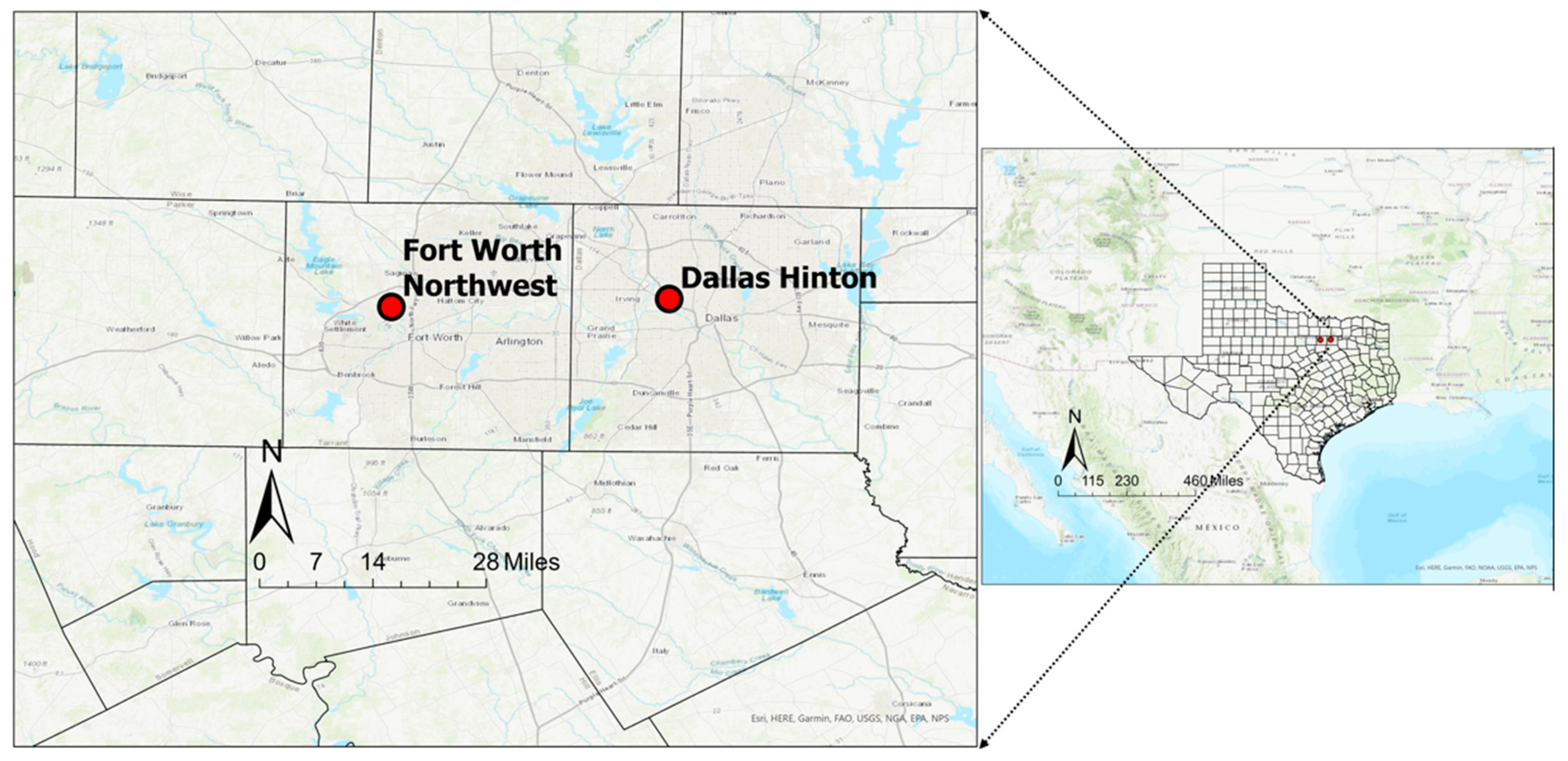
Figure 1. Geographical locations of Fort Worth Northwest (CAMS 013) and Dallas Hinton (CAMS 0161) sites.
Applsci 15 11923 g001
Figure 2. Architecture of an LSTM module, showing forget, input, and output gates.
Applsci 15 11923 g002
Figure 3. Architecture of a GRU module, showing reset and update gates.
Applsci 15 11923 g003
Figure 4. Architecture of the hybrid model.
Applsci 15 11923 g004
Figure 5. Temporal variations in ozone, NOx, and VOCs alongside meteorological parameters (OT, SR, and DP) during the model training period (2014–2020). The solid line denotes the mean, while dashed lines represent ±1 standard deviation over the entire period.
Applsci 15 11923 g005
Figure 6. (a) Monthly and (b) diurnal variations in NOx, ozone, and VOC in CAMS 013 during the training period. The dots are the mean concentrations and the bars are the standard deviations.
Applsci 15 11923 g006
Figure 7. (a,c) Monthly and (b,d) diurnal variations in OT, RH, and WS in CAMS 013 during the training period. The dots are the mean concentrations and the bars are the standard deviations.
Applsci 15 11923 g007
Figure 8. Heatmap of the correlation matrix between the variables.
Applsci 15 11923 g008
Figure 9. Feature importance of independent variables over a dependent variable. (a) Summary of the mean absolute impact. (b) Impact of each datapoint on the model.
Applsci 15 11923 g009
Figure 10. Correlation between observed and predicted 8 h ozone for CAMS 013 with best fit line; R2 value for years from 2021 to 2023.
Applsci 15 11923 g010
Figure 11. Time series forecast for high ozone concentration months: (a) June 2021, (b) May–June 2022, and (c) August–September 2023 for CAMS 013.
Applsci 15 11923 g011aApplsci 15 11923 g011b
Figure 12. Correlation between observed and predicted 8 h ozone for CAMS 0161 with best fit line; R2 value for years from 2015 to 2019.
Applsci 15 11923 g012
Figure 13. Time series forecast for high ozone concentration months: (a) July–August 2015, (b) June 2016, (c) August–September 2017, and (d) June–July 2018 for CAMS 0161.
Applsci 15 11923 g013aApplsci 15 11923 g013b
Table 1. Statistical summary of model training variables at CAMS 013.
PollutantsMeanStd. Dev.MedianMinMaxSkew
Ozone27.1415.4825.980.00113.910.53
NOx10.8315.026.060.00269.304.02
VOC25.6628.9716.682.31928.395.64
Meteorological Parameters
OT67.0917.1569.0412.82109.43−0.36
SR0.270.390.010.001.471.30
DP51.1316.2555.52−8.1176.89−0.66
RH60.5019.9761.269.3898.73−0.13
WD19.3110.0816.360.0979.842.22
WS7.524.097.000.0631.311.05
PWG15.227.1914.600.3075.470.69
VOC Species Concentrations
1,3-Butadiene0.040.040.030.001.004.52
1-Butene0.070.060.060.002.979.43
1-Pentene0.020.040.020.002.0516.84
2,2-Dimethylbutane0.030.030.020.001.288.57
Acetylene0.420.460.310.0024.4010.04
Benzene0.140.120.110.002.533.44
Cyclohexane0.070.070.050.002.073.90
Cyclopentane0.060.060.040.002.537.36
Ethane12.6718.777.300.74803.459.66
Ethylene0.740.850.480.0015.944.11
Isobutane0.900.930.620.0027.334.33
Isopentane1.121.360.750.0063.2110.31
Isoprene0.070.110.030.002.384.05
m/p Xylene0.110.150.070.005.376.70
n-Butane2.413.071.530.02133.369.01
n-Decane0.020.020.010.001.016.90
n-Heptane0.090.090.060.006.078.29
n-Hexane0.250.250.180.006.984.45
n-Nonane0.020.020.020.001.3012.17
n-Octane0.030.040.020.003.5019.75
n-Pentane0.760.760.530.0429.825.44
Propane4.895.253.150.1384.533.36
Propylene0.280.260.200.009.314.35
Toluene0.350.550.220.0068.3639.77
trans-2-Butene0.040.070.030.004.6724.34
trans-2-Pentene0.040.090.020.004.9718.01
Table 2. Summary of training hyperparameters and validation protocol.
ComponentValue
OptimizerAdam (β1 = 0.9, β2 = 0.999, ε = 10−7)
Learning rate0.002
LossMSE
Reported metricsRMSE, MAE, R2
Batch size64
Max epochs100
Early Stoppingmonitor = val_loss; patience = 10; restore_best_weights = True
ShuffleTrue (each epoch)
InitializationGlorot uniform (default)
Feature scalingMin–Max [0, 1] (features and target)
PCASeven components on scaled features
Table 3. Year-wise performance metrics of the hourly ozone forecasting model at CAMS 013.
YearMSERMSEMAEMBEIoA
202124.814.983.60−0.480.97
202229.235.403.88−0.370.97
202332.935.784.18−0.590.96
Table 4. Performance comparison of the hybrid surface ozone forecasting model for multiple years for CAMS 0161.
YearMSERMSEMAEMBEIoA
201530.375.514.09−0.430.97
201632.445.694.20−0.650.96
201731.205.584.14−0.130.96
201831.565.624.20−0.910.96
201933.595.804.30−1.070.95
Disclaimer/Publisher’s Note: The statements, opinions and data contained in all publications are solely those of the individual author(s) and contributor(s) and not of MDPI and/or the editor(s). MDPI and/or the editor(s) disclaim responsibility for any injury to people or property resulting from any ideas, methods, instructions or products referred to in the content.