Article

Extending Light Direction Reconstruction to Outdoor and Surface Datasets

1
Department of Computer Science and Mathematics, University of Applied Sciences Munich, Lothstr. 64, D-80335 Munich, Bavaria, Germany
2
Chair of Computer Graphics and Visualization, Technical University of Munich, Boltzmannstr. 3/II, D-85748 Garching, Bavaria, Germany
*
Author to whom correspondence should be addressed.
Appl. Sci. 2025, 15(23), 12779; https://doi.org/10.3390/app152312779
Submission received: 26 October 2025 / Revised: 16 November 2025 / Accepted: 26 November 2025 / Published: 3 December 2025
(This article belongs to the Special Issue Deep Learning Applications in Image Analysis)

Abstract

Immersive augmented reality (AR) requires consistent illumination between synthetic scene content and the real world. Recent deep neural networks achieve this by reconstructing important illumination parameters, though the performance was measured in clean laboratory environments. This study shows that the reconstruction performance of a recently proposed network architecture remains satisfying in more complex real-world outdoor scenarios. The labelled outdoor scenario dataset used in this study is provided as part of this publication. The study further reveals how auxiliary surface (in this scope, depth and normal vector) information affects the reconstruction performance of the network architecture.

1. Introduction

The registration problem in AR applications [1] describes the issue of achieving both consistent spatial placement of virtual content, known as the geometric registration problem, and coherent illumination between the real and synthetic world, known as the photometric registration problem. Diverging illumination between the real and the synthetic world may disrupt immersion in AR applications. When rendering virtual content in AR applications, it is important to apply suitable illumination parameters so that the virtual illumination resembles the real world situation. Immersion may be disrupted particularly easily, however, if the shading and the direction of cast shadows in the real and synthetic world significantly mismatch. In the past years, several deep neural network (DNN) approaches have been published to address this issue. Kán and Kaufmann [2] reconstructed the dominant light direction from red-green-blue-depth (RGB-D) images using a ResNet, yet figured that sole use of red-green-blue (RGB) data did not work for their approach. Miller et al. [3] modified the VGG-16 classification architecture [4] by introducing Net s x , s y , which regresses the direction of the dominant point light source in stereographic coordinates from RGB input and eliminated the need for additional depth information. Later, they improved the prediction performance of Net s x , s y by analysing its internal decision process [5], leading to architectural adjustments and an optimized synthetic training dataset.
Apparently, reconstructing the light direction is feasible both with regular RGB data and RGB data with additional depth information. Consider the reflective light term
f r ( x , ω i , ω o ) L i ( x , ω i ) ( ω i T n ) d ω i
of the rendering Equation [6], which incorporates the following components:
  • fr = bidirectional reflectance distribution function (BRDF);
  • Li = incident light radiance;
  • x = location to be lit;
  • ωi/ωo = incident/outgoing light direction;
  • Ω = entirety of ωi from the hemisphere above x.
The projective term (cyan) incorporates information about the reflective surface, particularly the angle between ω i and the orientation n of the surface. Commonly, n is represented by depth or normal vector information (hereafter referred to as surface information, which may generally include BRDF data but is explicitly excluded). This lets one assume that feeding additional surface data as auxiliary information to a network, though not essential, may ease the reconstruction task, as only f r and L i need to be estimated, which may help to achieve better reconstruction performance. RGB and depth information are sensor mappings of the same scene image and can be considered as multimodal data [7], which can be fed to a DNN either as early-, intermediate- or late-fusion. In this study, it is investigated whether the described multimodal data fusion indeed eases the illumination reconstruction task, leading to more precise illumination reconstruction.
Reconstruction approaches that are based on more recent computer vision architectures, such as ResNet [8] and ConvNeXt [9], perform slower or less accurate than Net s x , s y (Appendix A.1). Therefore, this study takes up the architectural adjustments suggested by Miller et al. [5], introducing the fully convolutional dense network (FCDN) architecture and evaluating its performance on the previously used test dataset T REAL . As T REAL , though containing real-world images, constitutes a benevolent dataset due to its photos taken under controlled lab conditions, the generalisability of FCDN is demonstrated by using a newly generated labelled outdoor dataset, which is published alongside this paper (https://sites.hm.edu/ccbv/projekte_6/projekte_detail_49024.de.html, accessed on 25 November 2025). While capturing real outdoor illumination conditions, the outdoor dataset is limited in that sense that the images of the dataset so far were recorded during high summer in Central Europe, meaning the images mostly depict cloudless, sunny scenes with little to no wind influence.
The main contributions of this study to the current state of scientific knowledge is summarized as follows:
  • Improvement of reconstruction error to 3.8 ° on reference test data via FCDN architecture.
  • Publishment of a labelled outdoor dataset suitable for illumination reconstruction that can be further expanded in the future.
  • Demonstration of the presented architecture’s ability to generalise to real scenarios (with rudimentary domain adaptation).
  • Investigation on whether multimodal (RGB-D, RGB-N) network architectures have any effect on the reconstruction performance.

2. Related Work

In the past, several DNN approaches to reconstruct illumination have been published, and they can be categorised into two research branches. Approaches in the first branch aim to generate illumination textures for image-based lighting (IBL) renderers by using DNNs to generate such textures directly or from reconstructed parameters to approximate illumination in indoor [10,11,12], outdoor [13,14] or both scenarios [15]. The second branch focuses on reconstructing specific illumination parameters, which is what this study targets.
Sommer et al. [16] employed a DenseNet-121 to reconstruct the illumination parameters { d , c , a , o } , with d being the direction towards the light source, c being the light colour, a being the ambient colour and o being the opacity value of a shadow casting texture, which is created pixel-wise by another fully connected DNN and used in their approach to generate soft shadows. The DenseNet-121 is trained on a modified variant of the Laval indoor HDR dataset [10], which is frequently used in IBL-based approaches, and receives RGB input images with a resolution of 256 × 192 . The approach requires the shadow casting DNN to be specifically trained for a certain model and is limited to planar shadow receivers. Providing an additional depth channel, Kán and Kaufmann [2] feed RGB-D images to a residual DNN and aim to predict the direction to the dominant light source in a given scene. The output light direction is given as a tuple of azimuth ϕ and elevation θ . The residual DNN is trained on synthetic RGB-D data and tested in real-world scenarios, resulting in an overall average error of 28.4 ° between the reconstructed light direction and the ground truth. Miller et al. [3] proposed a VGG-16-like Net s x s y to reconstruct the dominant light direction in stereographic coordinates from RGB images. They conducted experiments with Net s x s y being trained on solely synthetic, solely real and mixed data and determined that mixed training data performed the best with an average angular error of 7.1 ° on the used test dataset T real , which contained solely real-world indoor images. By analysing meta information, which arise as secondary data when applying explainable artificial intelligence (XAI) approaches, Miller et al. [5] derived the linear feature aggregation network (LFAN) and fully convolutional network (FCN) architectures, improving the average angular error when reconstructing the dominant light direction to 6.2 ° and 5.7 ° on the reference test set T real , respectively. Optimizing the synthetic training dataset, Miller et al. further improved the average angular error to 4.4 ° on T real with the proposed Net RTS , which is based on Net s x , s y . The input data is optimized by investigating the influence of synthetic training data, rendered with different illumination models and shadow algorithms, on the reconstruction performance. The best results were achieved with the Oren–Nayar [17] and Cook–Torrance [18] illumination models and ray-traced soft shadows [19], used in Net RTS . Combining the findings from architecture and dataset improvements, Miller et al. suggested adjustments to their proposed architectures to reduce potential over-fitting and rebuild its ability to generalise.

3. FCDN Evaluation on RGB Data

The FCN architecture [5] consists of the VGG-16 convolutional section C 1 to C 5 , which is extended by two convolutional blocks C 6 and C 7 to expand the extracted feature regions to the entire input image. Each additional block consists of one convolutional layer and a max-pooling operation. The entire convolutional section is followed by a single linear output layer L o . The FCN architecture, however, suffers from an inherent tendency to over-fit and presumed poor generalizability due to its inability to train well with augmented training data. Therefore, the FCDN architecture introduces a single dense layer D with a rectified linear unit (ReLU) activation function between C 7 and L o (Figure 1) to investigate if these adjustments overcome FCN’s architectural limits, as postulated by Miller et al. [5].
Like the training process of the predecessor models, the training of the FCDN architecture follows the two-phased Keras transfer learning and fine-tuning process. In the first phase, the model’s hyperparameters are optimized with KerasTuner [20] on a reduced dataset of 20,000 images over five epochs. In this phase, the convolutional section C 1 to C 5 is initialized with the weights of Net RTS as it showed best performance on T REAL . During the optimization process, the weights of C 1 to C 5 are not updated after each training epoch (the trainable flag is set to false). KerasTuner optimizes the filter size of C 6 and C 7 , the number of neurons of D, the dropout value, the learning rate, the batch size and the optimizer. In the second phase, the most promising variant is fine-tuned on the full dataset of 100,000 images for up to 250 epochs. During the fine-tuning training, the weights of C 5 are updated each epoch (trainable flag is set to true) and the learning rate is set to a tenth of the original rate, so C 5 gradually adjusts to the tail section and the new task. If the validation metric has not changed over a period of 12 epochs, the learning rate is reduced by a Keras learning rate reducer module. If the validation metric has not changed after another 20 epochs, the training is stopped early by a Keras early stopper module. In both phases, the datasets are split with a split ratio of 80:20 (ignoring rounding) for training and evaluation.
Miller et al. [5] used different datasets: one synthetic training and evaluation dataset DS syn from the same domain as the synthetic test dataset T syn , one real training and evaluation dataset DS real from the domain of the real indoor test dataset T real and several synthetic datasets that were generated with different illumination models. As combinations of synthetic and real data showed to produce the best results [3,5], the best-performing synthetic datasets ( DS syn and DS RTS ) described by Miller et al. [5] are mixed with DS real . Besides ImageNet [21], pre-trained base weights for C 1 to C 5 , base weights of Net s x s y and Net RTS are used in the transfer learning process. Each combination is used to train a dedicated FCDN model. Eventually, all FCDN models are evaluated on T real , revealing the model using pre-trained weights of Net s x s y and DS RTS to perform best with an average angular prediction error of 3.8 °  (Appendix A.4).

4. Real-World Generalisation

DNNs used to reconstruct illumination only provide real benefit if they perform satisfyingly under real conditions. To evaluate DNNs regarding their performance to generalise on real-world data, a test dataset of reasonable size is required. However, the major drawback of T real is its limited size. The Laval indoor HDR panorama dataset contains more than 2100 images and the Laval outdoor HDR panorama dataset [14] contains 205 images. Both datasets could be used to extend T real . Unfortunately, both Laval datasets are unlabelled, so labelled training images are not easily obtainable, especially from panoramas which do not clearly show the dominant light source, making most of the Laval indoor HDR panorama dataset and a quarter to half of the images in the Laval outdoor HDR dataset unusable for this purpose. Moreover, earlier iterations [3,5] were trained on data with anchor objects in the foreground, simulating common setups of AR environments. This particular image domain is not captured in the Laval datasets. In consequence, the proposed FCDN architecture needs to be trained on training data of similar domain, to remain comparable to earlier iterations. Hence, the Laval datasets are not suitable for this particular approach. T real could have been extended; however, indoor data generation would have required high levels of automation for both camera and light placement to effectively extend the dataset, which were not available.
Instead, a labelled outdoor dataset is generated, as the generation process for this kind of data can be performed by simply deploying a self-written data gathering application to a mobile device with a suitable camera and taking photographs in specified time intervals from an outdoor scene, which is illuminated by the sun, reducing the automation effort to measuring required references and placing the camera once a day. The image data used in this study is gathered mostly under fair weather conditions due to geographical and seasonal circumstances at the time and location of the recording. Cloudy weather conditions would cause the perceived illumination to be very diffuse and, thus, the light direction is difficult to determine from illumination effects under such weather conditions for both humans and the introduced DNN. Nevertheless, the introduced DNN aims to reconstruct the dominant light direction in a given scene that is illuminated by one main light source—ideally one point light source. Given that scenes with very diffuse illumination, e.g., under said conditions, do not have typical dominant light directions, the limitation of the outdoor dataset to mostly fair weather conditions does not constitute a problem for this study.

4.1. Recording Setup

The device is mounted to a tripod and focused on the captured scene. In the foreground of the scene, one or more different 3D-printed objects are placed on a table, which is covered by differently coloured tablecloths (Figure 2).
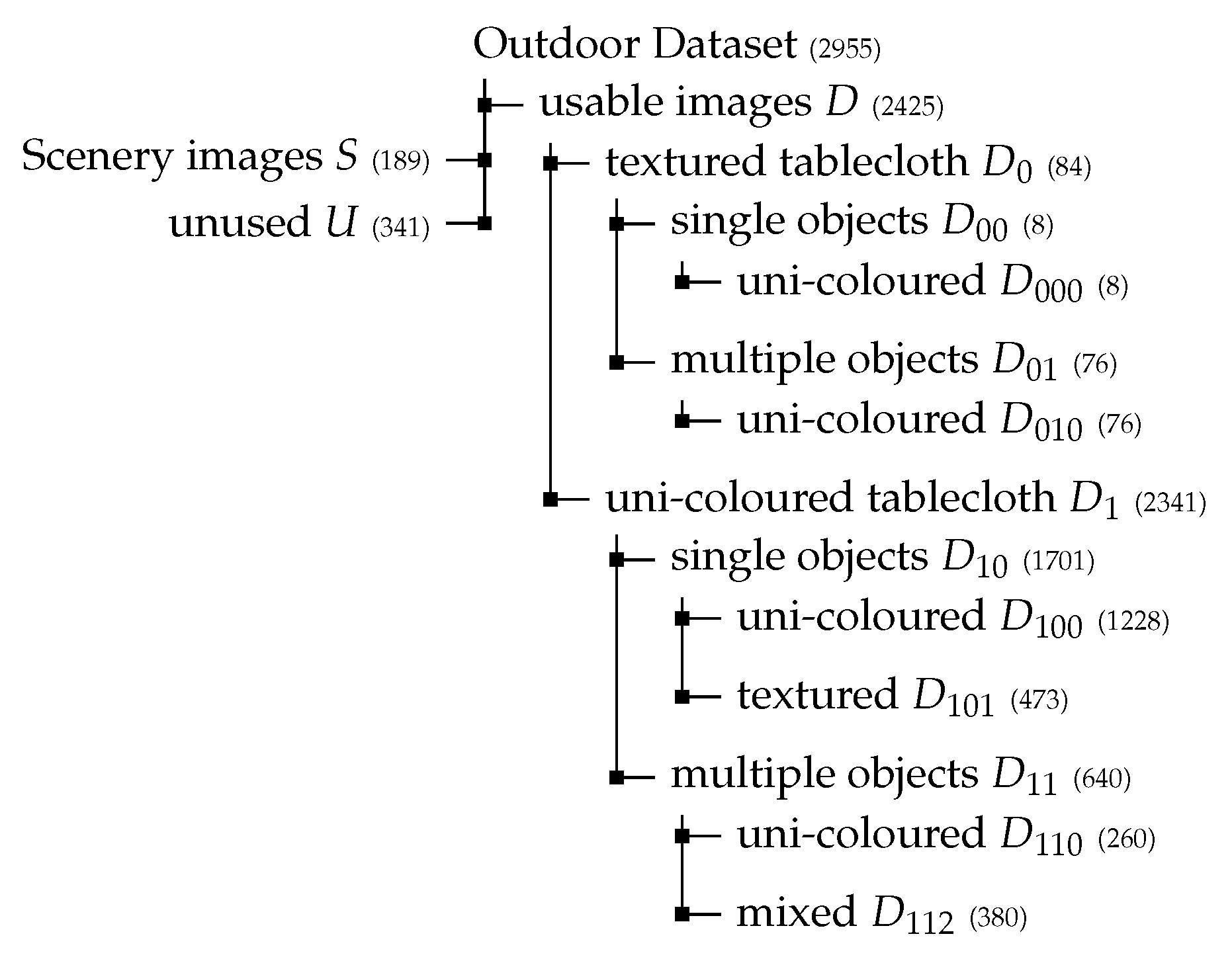
In the foreground scenes, five different models (a white Stanford bunny, a textured Stanford bunny, a white Stanford Buddha, a purple Stanford Buddha and a white Stanford dragon) and four different tablecloths (a yellow, a blue, a green and a textured one in a Bavarian style) are used. In total, 2955 images are captured and organised (Appendix A.2.3) into a usable fraction D of 2425 images, a fraction of landscape photos S with 189 images and a fraction U containing 341 unused images (e.g., the scene was fully shaded by a tree, the camera tripod was blown over by the wind or similar).
This dataset structure not only allows the investigation of how well DNN models generalise on real-world outdoor data, but also how robust those models are with respect to slight changes to the otherwise same domain.

4.2. Labelling Outdoor Photographs

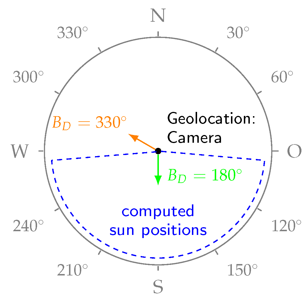
To label each image with the direction towards the light source, in this context the sun, the bearing in which the camera is pointing and the position of the sun is required. The position of the sun can be computed from a given point in time and the location on earth. The DNNs of previous approaches [3,5] assumed clockwise labelling with light directions originating from the left side in an image to be light azimuth angles of 90 ° and light directions coming from the opposite side of the scene (casting a shadow towards the camera) to be caused by light azimuth angles of 180 ° . In the context of earth locations and following this labelling convention, the computed sun’s position could be directly used as a label if the device’s orientation is facing southwards (Figure 3).
To capture scene images illuminated from as many light directions as possible, the images are taken with the device facing various cardinal directions, which needs to be incorporated in the labelling process. For this, the device’s bearing is required, which could be measured with a compass. However, determining the bearing with a compass or gyroscope sensor may not produce measurements accurate enough for the labelling process, due to scale resolution when reading a compass and technical inaccuracies of the gyroscope sensor. To increase the accuracy, the device’s bearing B D is computed between a distant ( 1.0   km to 1.4   km ) reference point P r , previously located with the global positioning system (GPS) sensor, and the device’s GPS location P d (Appendix A.2.1).
With B D and the sun’s azimuth and elevation, the actual image labels indicating the direction to the sun can be computed. As B D and the sun’s azimuth and elevation are given in the context of spherical coordinates, the dataset labels are computed in this representation and later converted into stereographic coordinates (as described in Miller et al. [3]). Since the elevation of the sun θ sun is independent from B D , θ sun can be directly assigned to the elevation label L θ . To compute the azimuth label L ϕ , the azimuth of the sun ϕ sun requires to be adjusted by B D (Appendix A.3.1), resulting in the final spheric label L ϕ , L θ , which is eventually converted into the stereographic label L s x , L s y . The ground truth labels of the dataset itself incorporate an inherent measurement error between 0.82 ° and 1.15 ° (Appendix A.2.2), which is important to keep in mind when evaluating a DNN’s performance.

4.3. Evaluation Strategy

Predicting illumination in an unknown domain is a difficult task. With high certainty, models trained on different domains, especially without any incorporated domain adaptation measures, are going to perform worse in unknown, more complex domains. With this in mind, each subset of the aforementioned dataset D with reasonable size is split into a test dataset and a training/validation dataset, intended to be used for an adaptation training process. Due to their small size, the data subsets S, D 001 and D 010 are used in their entirety in the test datasets T S , T D 001 and T D 010 . The remaining subsets are split into test subsets T x y and training/validation subsets D S x y with x y indicating the specifically matching subset (Table 1).
Before usage, the training/validation subsets D S Dxyz are split with a ratio of 80:20 into respective sets.
The adaptation training is performed using the FCDN architecture with ImageNet pre-trained weights for C 1 to C 5 . Different models are trained with specific training subsets or combinations to investigate the architecture’s ability to generalise in certain situations; for instance, how well a model that is trained for outdoor scenes with single objects performs on the aforementioned T REAL of indoor images, or on outdoor scenes with multiple objects. The training process is conducted as described earlier (Section 3, second paragraph).

5. Influence of Surface Data

Kán and Kaufmann [2] found their network to be unable to properly reconstruct the dominant light direction when only using RGB instead of RGB-D information. In contrast, Miller et al. [3] showed in their approach that it is possible to reconstruct the dominant light direction solely from RGB data. From a theoretical point of view, one can argue that a DNN is capable of performing an end-to-end transformation of the illumination situation, given by a single RGB image, to a directional vector representing the dominant light direction, but having additional information about the shape of the surfaces in the RGB image may help to ease the task of doing so. Considering the incidental light part of the reflective light term (Equation (1), cyan part) in the rendering Equation [6], the angle between the orientation of the surface, denoted by the normal vector n, and the light inciding from a certain direction ω i determines how much light from ω i is actually received at the investigated location x. So, when trying to reconstruct the dominant light direction, a DNN is trying to map the reflected light L o of each pixel visible in the input image to the most significant inciding light direction ω i without knowledge about each pixel’s material ( f r ), radiance ( L i ) and surface (n). Considering the mentioned surface orientation term ω i T n , it is a reasonable attempt to improve a DNN’s prediction result by providing additional information about the orientation of the surface, either as depth information from a sensor or as normal vector information, which may be reconstructable, yet non-trivially, from depth data [22]. With the provided surface orientation information, a DNN would only have to estimate values for f r and L i when reconstructing the dominant light direction. This study investigates if providing additional surface information indeed improves the prediction performance or if DNNs may inherently learn surface structures, not requiring additional information input, when confronted with a light direction reconstruction task. The investigation is conducted on synthetic data, as the labels of this data do not incorporate any measurement errors. Further, additional surface information is not expected to improve the reconstruction performance in real-world scenarios if it does not improve the results under synthetic laboratory conditions.

5.1. Fusing Data

Surface information, either as depth or normal vector data, can be passed to a DNN either as early, late or intermediate fusion (Figure 4).
In intermediate and late fusion settings, the feature extraction needs to extract meaningful information in respect to the data sample label only from surface information. However, since the shape of the surface is not influenced by light angles, surface information is entirely independent from illumination and, therefore, a DNN in principle cannot infer illumination from surface information alone, as empirically confirmed. By fusing colour and surface information right after the input layer in an early fusion approach, meaningful features are extracted from both multimodal sensor data, so that the decision part may infer the direction to the dominant light source more accurately. After passing the data augmentation stage, which applies random zoom and shifting to both information types and random brightness to the colour features, colour and surface information are concatenated and eventually passed to the first convolutional layer of the DNN, leading to a kernel depth from three (RGB only) to four in case of RGB-D and six for red-green-blue-normal (RGB-N) information, respectively.

5.2. Training with RGB-D and RGB-N

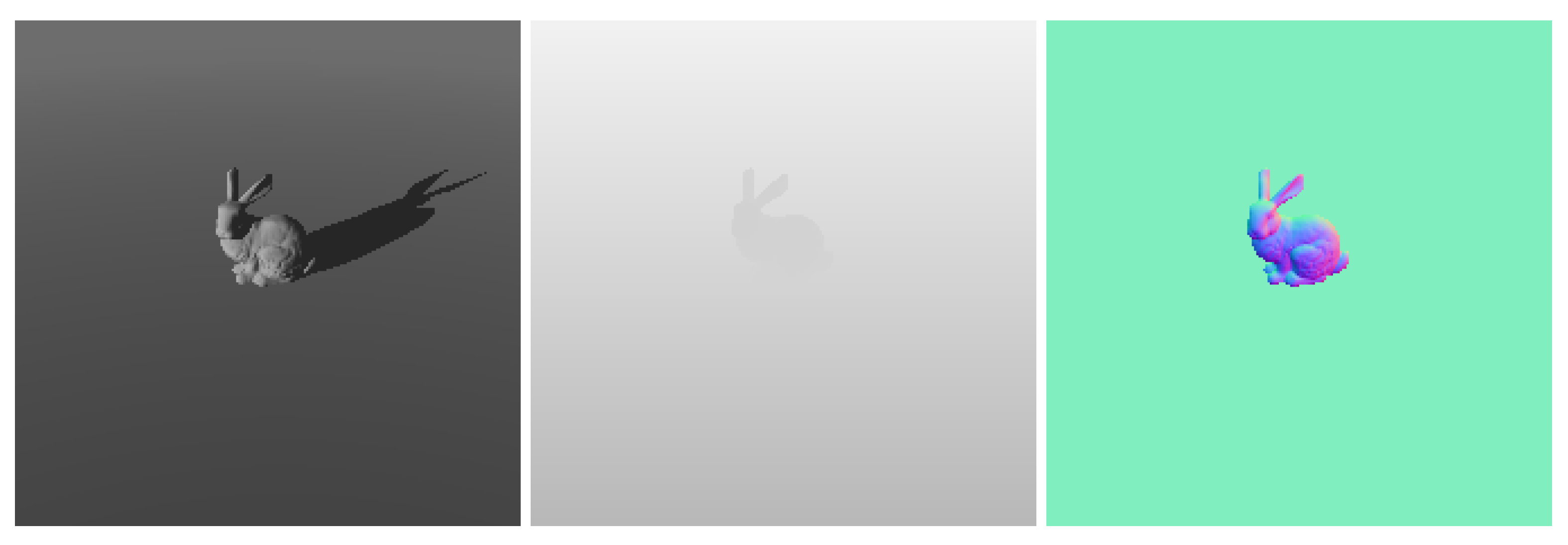
To investigate the influence of surface information on the prediction performance, DNNs of the aforementioned FCDN architecture are trained for RGB-D and RGB-N information with laboratory data, i.e., synthetic data (80,000 for training, 20,000 for validation and 10,000 for testing) with depth and normal information, and compared to a baseline FCDN network Net base , which uses pre-trained weights of Net RTS and is trained solely on RGB information. Since multimodal input features require all layers to be trained, all layers beginning with C 1 in Net base are trained, which differs from the described training procedure (Section 3). Throughout all datasets, the RGB information remains the same and is rendered with the parameters of the best-performing dataset DS RTS from Miller et al. [5]. In summary, three datasets are compiled, consisting of solely RGB information ( SDS RGB ), RGB-D information ( SDS RGB-D ) and RGB-N information ( SDS RGB-N ). Corresponding test datasets are called T SDS without additional surface data indication, as this information can be derived from the context. Depth and normal information is generated simultaneously with the RGB information and stored in separate files, containing information as viewed by the recording camera (Figure 5).
Before being stored into a file, the normal information is packed into an interval of [ 0 ,   1 ] (Appendix A.3.2). When being passed to a DNN, the normal information remains unconverted, as converting it back into an interval of [ 1 ,   1 ] would most likely lead to incompatibility in regards of the used ReLU activation function, considering the range [ 0 ,   1 ] of RGB data, which the normal data is supposed to be merged with. Apart from that, normal data is usually computed from depth data, commonly recorded by depth sensors, and may consequently be mapped into the interval [ 0 ,   1 ] while doing so.
To profit from pre-trained model weights in the given early fusion setup, the weights of the convolutional section in Net RTS are loaded into C 1 to C 5 . However, these pre-trained models do not possess weights for additional layer weights that are required to process the concatenated surface information of the input. Facing a similar problem in a near-infrared (NIR) context, Liu et al. [23] initialized missing layer weights with the average of existing RGB weights. Yet, NIR is more closely related to RGB than surface information, leaving random initialization as another approach. Both methods are investigated, yet average initialization consistently ranked behind random initialization. The weights in the remaining layers are initialized randomly.
Hyperparameters commonly influence the prediction performance of DNNs significantly. Thus, two hyperparameter strategies S A and S B are investigated to isolate the effects of additional surface information on the reconstruction performance. The first strategy S A uses the same hyperparameters as Net base to solely investigate the influence of additional surface information. This favours RGB information, as feature extraction and decision making section are not adapted to additional surface information. Consequently, strategy S B optimizes the full range of hyperparameters: the optimizer, the learning rate, the batch size, the filter size of C 6 and C 7 , the number of neurons in the dense layer, the dropout rate and whether to use a bias in the output layer, allowing all layers to adjust to the additional surface information.
In addition to the transfer learning methods used to train Net FCD , the fine-tuning is conducted with an unmodified learning rate to gain further insights and to rule out possible unnoticed side effects when investigating only one of these methods. For instance, the effect sizes could be below the significance level if investigated only with a reduced learning rate.

5.3. Statistical Investigation

The comparison between surface information models and Net base on the same test samples constitutes a test with paired samples. Therefore, to determine whether surface information improves the average illumination reconstruction error, Wilcoxon signed-rank tests [24] between the multimodal FCDN models and Net base are conducted with a significance level of α = 0.01 . However, due to the large sample size of the test dataset (10,000 samples), the test is likely to show significant differences between the multimodal FCDN models and Net base . Thus, the Pearson correlation coefficient r [25] is computed in addition, to determine the effect size | r | and its classification [26] in small, medium and large effect sizes (Appendix A.3.3) as a more descriptive metric. In that sense, the effect size tells how strongly surface information is influencing the illumination reconstruction performance.
Those tests and factors, however, do not reflect if certain multimodal FCDN models may have higher average prediction errors but in return may suffer less from extreme statistical outliers. Therefore, the resulting error distributions are additionally investigated with box plots.

6. Results

In this section, results regarding the FCDN architecture performance, the generalisability on real outdoor data and the effects of surface information on the reconstruction performance are presented.

6.1. Results: FCDN Architecture

The earlier published reference DNNs Net s x , s y [3], LFAN, FCN and Net RTS [5], to which the FCDN architecture is compared, achieved average angular errors e on T real of 7.1 ° , 6.2 ° , 5.7 ° and 4.4 ° (Table 2, upper section), respectively.
The lowest e = 3.8 ° is achieved by the FCDN architecture Net F C D (Table 2, lower section) trained with a combination of DS RTS and DS real and pre-trained base weights from Net s x , s y . Net F C D uses 1205 filters in C 6 and 2466 filters in C 7 . The dense layer D contains 4769 neurons and a dropout rate of 0.1 is applied. The output layer L o does not use a bias. A Nadam optimizer is used with a learning rate of 3.6 × 10 5 and the dataset is chunked into batches of size 16.
Considering the distributions of e (Figure 6) achieved by Net s x , s y , LFAN, FCN, Net RTS and Net F C D , the error range of each distribution gets narrower with each architectural adjustment.

6.2. Results: Outdoor Data Generalisation

As expected, the selection of unadapted models ( Net s x , s y , Net RTS and Net F C D ) achieved unsatisfying prediction performance (Table 3, upper section) on the outdoor test datasets with angular errors e between 44.4 ° and 65.7 ° .
Investigating the generalisability of the FCDN architecture (Table 3, lower section), Net DS D 10 , trained on images of D S D 10 (single textured and uni-coloured objects on uni-coloured surfaces), achieved 5.0 ° on the respective test dataset T D 10 , though did not perform satisfyingly on T D 11 (multiple objects—uni-coloured and mixed—on uni-coloured surfaces), T D 0 (single and multiple uni-coloured objects on textured surface), S (scenery images) and T REAL . Adding DS REAL to the training data in Net DS REAL + DS D 10 , its prediction error improved to 4.8 ° on T D 10 and 7.0 ° on T REAL , yet remained unsatisfying on the remaining test datasets. Net DS REAL + DS D 10 / D 11 , trained with D S D 10 , D S D 11 and DS REAL , eventually achieved 5.8 ° on T D 10 , 5.7 ° on T D 11 and 6.7 ° on T REAL , but did not perform satisfyingly on T D 0 and S. Further adjustment trainings for the domains of T D 0 and S have not been conducted due to small dataset sizes.

6.3. Results: Effects of Surface Data

When investigating the influence of surface information (Table 4), the baseline DNN Net base achieved an error e of 0.9 ° .
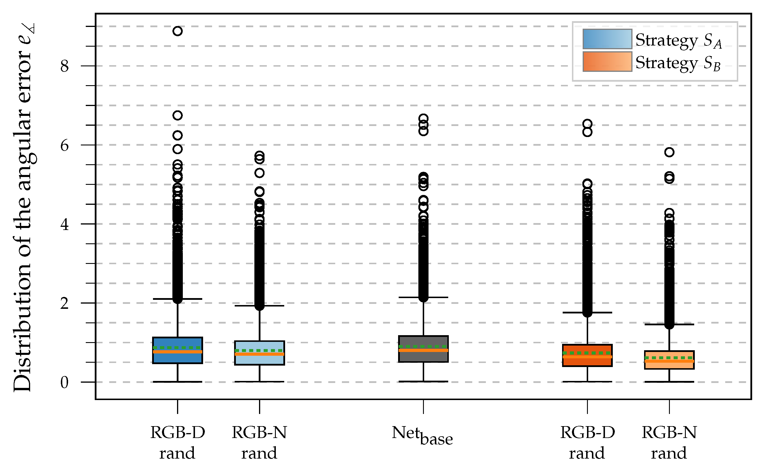
Applying S A , the RGB-D experiment yielded a significant ( p < α ), yet negligible (effect size | r | < 0.1 ) difference. The RGB-N experiment achieved a significant difference ( p < α ) with a small effect size of | r | = 0.167 . The RGB-D and RGB-N experiments applying S B both yielded significant differences ( p < α ) with RGB-D showing a small effect size with | r | = 0.281 and RGB-N showing a medium effect size of | r | = 0.461 . This behaviour is reflected in the distribution of the angular error e (Figure 7):
Graphs of the RGB-N experiments appear notably narrower with less pronounced outliers than graphs of the RGB-D experiments compared to the grey graph of Net base .
The described results are based on experiments with randomly initialized missing multimodal pre-trained weights. Further, only the results of the transfer learning method with unmodified learning rate are depicted, as the modified learning rate results showed the same behaviour with higher e . Additional results can be found on the project’s webpage.

7. Discussion

The average angular prediction error e indicating the dominant light direction in a scene could be improved to 3.8 ° on T REAL with Net FCD . In known domains, the FCDN architecture performs satisfyingly, even under real-world conditions as demonstrated on T REAL and the real outdoor test datasets. However, it is limited in principle on unknown domains (for instance, Net DS D 10 achieved 5.0 ° on images with single objects on uni-coloured surfaces but deteriorated to 36.3 ° on images with multiple objects on the same surface) as it does not incorporate domain adaptation mechanisms. Adding the dense Layer D did not seemingly contribute to improve this issue either.
To put the achieved angular errors on the real outdoor and on the synthetic RGB laboratory datasets into perspective, one needs to consider that the labels of the outdoor dataset incorporate measurement errors, whereas a similar error is in principle not present in the labels of the synthetic laboratory dataset. Therefore, the achievable minimum error on synthetic test data can be in principle lower than on real-world data with measured label information. The minimum measurement error in the outdoor dataset labels is estimated to lie between 0.82 ° and 1.15 ° (Appendix A.2.2). Due to geographical limitations at the place of recording, the dataset is missing data points of light inclining from the north-eastern sky region. So far, the dataset does not contain images that were taken under cloudy or rainy weather conditions as the dataset was gathered during high summer in Central Europe. The missing weather conditions are no issue for this study, as the proposed DNN aims to reconstruct the direction to a dominant point light source. The missing weather conditions need to be recorded in a future dataset extension. Nonetheless, the outdoor dataset contains a small number of images that show the scene to be partially or fully shaded by a single cloud, a tree or other light obstacles.
So, does surface information improve the light direction prediction performance? It does, yet with a low impact. The experiments with depth information showed small effect sizes at best, making additional depth information in relation to the expected performance gain not worth the additional effort. Adding normal vector information resulted in small to medium effect sizes and less pronounced outliers. Considering the effort required to achieve normal vector information, however, their impact on the performance gain may be too small to be practically applicable. Given that these results were achieved under laboratory conditions, we would not recommend incorporating additional surface information when aiming to improve the prediction performance as, considering the complexity, their impact is expected to be even lower under real conditions.

Summary

In summary, the proposed architectural changes of the FCDN architecture were partially successful. With almost 3000 labelled images, the generated outdoor dataset constitutes a good foundation to extend the presented work. Since each image is labelled with a variety of recorded information, such as METAR data and weather data, the dataset could be useful in other scientific disciplines, too. The investigation of the influence of surface information clarified that the additional required computing power outweighs the benefits of adding additional surface information.
The real outdoor dataset is publicly available (https://sites.hm.edu/ccbv/projekte_6/projekte_detail_49024.de.html). Source code for the DNN and the data gathering application along with documentation is also available there, so the software may be used by the community to create their own datasets. Detailed information about the dataset and further details on the results can be found on the project webpage as well.

8. Future Work

In the future, we intend to gradually extend the labelled outdoor dataset provided with this study with images from different places on earth with different weather conditions to offer a large labelled dataset that can be used to teach deep neural networks how to reconstruct illumination parameters. It would be interesting to see, if the proposed architecture—with specific domain adjustment training—is able to reconstruct the dominant light direction in cloudy or rainy weather situations. Since software and documentation is publicly available, this idea could also benefit from community participation.
The prediction performances of the investigated networks are prone to unknown domains. Introducing mechanisms that enable the networks to adapt to unknown domains in some way could reduce the effort required to tailor training datasets and increase the performance on unknown data overall. Adaptation to unknown domains could be achieved by training an encoder to produce core features from synthetic and real images and having a discriminator to decide whether the produced core features originate from synthetic or real images. Once the origin of the core features is indistinguishable, they may be used in a succeeding dense section to derive illumination parameters from it.
Considering illumination reconstruction from scenery images (S), it may be interesting to investigate if a specifically trained FCDN instance may perform well or if this particular problem may be an entirely new research topic, as scenery images may incorporate a whole new range of perturbing effects, such as shadows from invisible objects like clouds. In this context, the further investigation of methods that are capable of reconstructing more complex illumination parameters to approximate these illumination conditions may be an interesting research topic.
Most illumination reconstruction approaches are compared based on how accurate they reconstruct a light position or direction. However, from what we could find, it is unclear how accurately reconstructed illumination parameters have to resemble real-world illumination situations to successfully deceive human perception. We, therefore, intend to conduct a study in the near future to quantify the noticeable deviation of illumination effects.

Author Contributions

Conceptualization, all authors; methodology, all authors; software, M.M. and J.A.; validation, all authors; formal analysis, J.A. and M.M.; investigation, M.M. and J.A.; resources, A.N.; data curation, M.M.; writing—original draft preparation, M.M. and J.A.; writing—review and editing, A.N. and R.W.; visualization, M.M. and J.A.; supervision, A.N. and R.W.; project administration, A.N.; funding acquisition, A.N. All authors have read and agreed to the published version of the manuscript.

Funding

This research received no external funding.

Institutional Review Board Statement

Not applicable.

Informed Consent Statement

Not applicable.

Data Availability Statement

The data and other material used in this study can be found at https://sites.hm.edu/ccbv/projekte_6/projekte_detail_49024.de.html (accessed on 25 November 2025).

Acknowledgments

We would like to thank Hubert Pihale for granting us access to his meadow on which we placed the camera setup to create the outdoor dataset. Andreas Zielke (https://hm.edu/kontakte_de/contact_detail_834.de.html), Tobias Höfer and Eduard Bartolovic provided valuable advice and feedback, for which we are very grateful. Eventually, special gratitude is due to Conrad Smith for his repeated help with questions regarding linguistic matters. We used GPT 3.0 and 4.0 here and there to suggest expressions and rephrased those suggestions to our liking.

Conflicts of Interest

The authors declare no conflicts of interest. The funders had no role in the design of the study; in the collection, analyses, or interpretation of data; in the writing of the manuscript; or in the decision to publish the results.

Abbreviations

The following abbreviations are used in this manuscript:
ARaugmented reality
BRDF bidirectional reflectance distribution function
DNNdeep neural network
FCDNfully convolutional dense network
FCNfully convolutional network
GPSglobal positioning system
IBLimage-based lighting
LFANlinear feature aggregation network
NIRnear-infrared
ReLUrectified linear unit
RGBred-green-blue
RGB-Dred-green-blue-depth
RGB-Nred-green-blue-normal
XAIexplainable artificial intelligence

Appendix A

In this section additional material related to the study can be found.

Appendix A.1. Reconstruction Performance of Recent Architectures

Net FCD is an optimised version of the Net s x , s y , which is based on the VGG-16 architecture. This base architecture was chosen due to its good inference performance in relation to the required computational workload. However, one could argue that recent architectures offer superior performance and throughput.
Therefore, different models that incorporate the feature extraction sections of recent architectures, which are extended by a custom dense section, are optimised and trained. The first layer of the custom dense section is a flatten layer. Depending on a hyperparameter that determines whether to use batch normalization, the flatten layer is followed by a respective layer. After that, a cascade of d dense blocks is attached, in which d is defined by a hyperparameter, ranging from 1 to 3. The number of neurons n 0 in the first dense block is also defined by a hyperparameter, ranging from 64 to 6144 . In each cascade step, the number of neurons is halved. In the dense layer of each dense block, a global dropout hyperparameter, ranging from 0.1 to 0.9 , and a ReLU activation function are used. Depending on the batch normalization hyperparameter, the dense layer in a dense block may be followed by a batch normalization layer. Eventually, the custom dense section is completed by a linear output layer with two neurons and a hyperparameter that determines whether to use a bias in this layer or not. Further hyperparameters define the batch size (choosing from a set of sizes s with s = { 16 , 32 , 64 } ) the optimizer (choosing from a set o with o = { Adam , Nadam , RMSprop } ) and the learning rate, ranging from 1 × 10 1 to 1 × 10 6 . The performance and inference time of those new models is then compared to Net s x , s y (Table A1).
Table A1. Results of different illumination reconstruction models based on recent computer vision architectures. The DNNs are trained on the same training datasets that correspond to T REAL and T SYN [3]. T D 10 and T D 11 are introduced in this study.
DNN T REAL T SYN T D 10 T D 11
Avg. e Avg. Time Avg. e Avg. Time Avg. e Avg. Time Avg. e Avg. Time
Net s x , s y 7.1 ° ≈6 ms 3.3 ° ≈2 ms 54.2 ° ≈2.5 ms 45.9 ° ≈3.5 ms
ResNet 50 s x , s y 13.7 ° ≈17 ms 10 ° ≈6 ms 100 ° ≈7 ms 82 ° ≈9.5 ms
ConvNeXt-T s x , s y 12.6 ° ≈33.1 ms 5.9 ° ≈12.1 ms 54.5 ° ≈14.2 ms 47.9 ° ≈18 ms
ConvNeXt-B s x , s y 6 ° ≈54.6 ms 3 ° ≈22.5 ms 37.2 ° ≈25.5 ms 34.8 ° ≈32.6 ms
The comparison is conducted on a Nvidia RTX 4090 GPU in a native Windows Tensorflow 2.10 environment using the test datasets T REAL , T SYN (both from Miller et al. [3]), T D 10 and T D 11 .

Appendix A.1.1. ResNet50sx,sy Details

The trained ResNet 50 s x , s y uses a batch size of 64, RMSProp as optimizer and a learning rate of 1 × 10 1 . It incorporates batch normalization layers and does not use an output layer bias. It uses two dense blocks with a 64 neurons in the first cascade. The dropout rate used in the dense section is 0.1 . During the fine-tuning phase of the transfer learning process, the last convolutional block, beginning with layer 143 is set to be trainable.

Appendix A.1.2. ConvNeXt-Tsx,sy Details

The trained ConvNeXt-Tsx,sy uses a batch size of 64, RMSProp as optimizer and a learning rate of 7.8 × 10 4 . As the keras implementation of ConvNeXt provides a flag, which determines whether to incorporate a special preprocessing layer, the usage in the training process is determined by a hyperparameter. The hyperparameter optimization advises not to use this preprocessing layer. The DNN incorporates batch normalization layers and does not use an output layer bias. The custom dense section contains three dense blocks with 64 neurons in the first cascade. The dropout rate is 0.1 and in the fine-tuning phase of the transfer learning process each layer of the ConvNeXt feature extraction beginning with layer 125 is set to be trainable.

Appendix A.1.3. ConvNeXt-Bsx,sy Details

Due to memory limitations, the range upper bound of n 0 in the first dense block had to be reduced from 6144 to 4096 . As the tiny version before, the trained ConvNeXt-Bsx,sy uses a batch size of 64 and RMSProp as optimizer, though a learning rate of 0.1 . The preprocessing layer is not used. The DNN uses batch normalization and a bias value in the output layer. The custom dense section uses one single block with 64 neurons. The dropout rate is 0.1 . In the fine-tuning phase, the third feature extraction stage beginning with layer 269 is set to be trainable.

Appendix A.1.4. Comparison Conclusion

Each of the recent architectures shows significantly higher inference times when reconstructing light directions from test images. At the same time, only the tested ConvNeXt-Bsx,sy could achieve slightly better reconstruction performance than Net s x , s y , though roughly ten times slower, and is therefore not applicable in real-time scenarios anymore. Consequently, these results highlight the relevance of Net FCD for the task of reconstructing the dominant light direction from an RGB images in comparison to more recent architectures.

Appendix A.2. Outdoor Dataset Material

This section contains additional material related to the recorded outdoor dataset.

Appendix A.2.1. Computation of Bearing

Considering the short distances to visible reference locations, the initial bearing formula is employed to compute B D :
X = cos P r lat   · sin P r lon P d lon
Y = cos P d lat   ·   sin P r lat sin P d lat   ·   cos P r lat   ·   cos P r lon P d lon
B D = arctan 2 X , Y

Appendix A.2.2. Ground Truth Error Estimation

Assuming a GPS error of about 10   m per measurement and the distance D P d P r between the reference point P r and the device’s location P d , computed with the Haversine formula
u = sin P r lat P d lat 2 2
v = cos P d lat   ·   cos P r lat   ·   sin P r lon P d lon 2 2
D P d P r =   2   ·   R e   ·   arctan 2 u + v , 1 ( u + v )
and R e being the Earth’s radius, an estimation of the angular measurement error ε of B D can be computed with
ε = arctan 20   m D P d P r
given that difficultly measurable factors, such as wind and thermic effects on the tripod and attached items, may also influence ε . Furthermore, ε varies throughout the dataset, as D P d P r is dependent on P r , whose distance to P d in the current dataset ranges from ≈1 km to ≈1.4 km. Hence, the GPS-induced minimum value of ε ranges from 0.82 ° to 1.15 ° . Further effects on ε are not quantifiable due to their random occurrence, meaning gusts of wind or the combination of thermal effects on the material and the condition of the ground surface, on which the camera tripod is placed.
The height above sea level is usually considered in computations that require high precision, for instance in astronomic calculations or when calibrating astronomic optics. Due to its minor influence compared to other factors of the setup, like its susceptibility to wind, the height above sea level is disregarded in these computations.

Appendix A.2.3. Dataset Organisation

The images of D are organised (Figure A1) in images showing a table with textured tablecloth D 0 and with uni-coloured tablecloth D 1 . These subsections are then further divided into images displaying single objects ( D x 0 ) and images showing multiple objects ( D x 1 ). On the third and last division layer, images are grouped depending on the surface appearance of the objects: uni-coloured objects: D x x 0 ; textured objects: D x x 1 ; and mixed objects: D x x 2 .
Figure A1. Organisation of the outdoor dataset. The number of images is given in parentheses. Empty branches are not depicted.
Applsci 15 12779 g0a1

Appendix A.3. Supplementary Math

In this section, additional formulas and equations are provided, as well as how the effect size used for the statistical evaluation was classified into three groups.

Appendix A.3.1. Azimuth Label Adjustment

The azimuth label L ϕ is computed by adjusting the azimuth of the sun ϕ sun by the device’s bearing B D using
ϕ D = ϕ sun + ( 180 B D ) if   B D 0 ϕ sun ( 180 + B D ) else
L ϕ = ϕ D   mod   360 if   ϕ D 0 ( 360 ϕ D )   mod   360 else

Appendix A.3.2. Packing Operation for Normals

Normal information n = n x , n y , n z T with n x , n y , n z [ 1   , 1 ] is packed from an interval of [ 1 ,   1 ] into an interval of [ 0 ,   1 ] using
n T = n 2 + 0.5

Appendix A.3.3. Effect Size Classification

The effect size | r | was classified into one of three interval classes (Table A2).
Table A2. Effect size classification.
0.1 | r | < 0.3 small
0.3 | r | < 0.5 medium
| r | 0.5 large

Appendix A.4. Supplementary Results

In this section more detailed results data are provided.

FCDN Architecture Results

Trained on a mix of DS syn and DS real , the FCDN architecture achieved average angular errors e on T REAL (Table A3) of 4.0 ° , 4.8 ° and 4.2 ° with pre-trained ImageNet, Net s x , s y and Net RTS base weights, respectively. It further achieved 4.0 ° , 3.8 ° and 4.6 ° , respectively, when being trained on a mix of DS RTS and DS real .
Table A3. Results of mixed trained FCDN models on T REAL with best performance ( Net FCD , bold). Entries in the column synthetic Dataset indicate which specific dataset was combined with DS real .
Synthetic ContributionBase Weights
ImageNet Net s x , s y Net RTS
DS syn 4.0 ° 4.8 ° 4.2 °
DS RTS 4.0 ° 3.8 ° 4.6 °

References

  1. Kanbara, M.; Yokoya, N. Geometric and photometric registration for real-time augmented reality. In Proceedings of the International Symposium on Mixed and Augmented Reality, Darmstadt, Germany, 1 October 2002; pp. 279–280. [Google Scholar] [CrossRef]
  2. Kán, P.; Kaufmann, H. DeepLight: Light Source Estimation for Augmented Reality using Deep Learning. Vis. Comput. 2019, 35, 873–883. [Google Scholar] [CrossRef]
  3. Miller, M.; Nischwitz, A.; Westermann, R. Deep Light Direction Reconstruction from single RGB images. In Proceedings of the 29 International Conference in Central Europe on Computer Graphics, Visualization and Computer Vision: Full Papers Proceedings, Plzen, Czech Republic, 17–21 May 2021; Computer Science Research Notes. pp. 31–40. [Google Scholar] [CrossRef]
  4. Simonyan, K.; Zisserman, A. Very deep convolutional networks for large-scale image recognition. In Proceedings of the 3rd International Conference on Learning Representations, ICLR 2015: Conference Track Proceedings, San Diego, CA, USA, 7–9 May 2015. [Google Scholar] [CrossRef]
  5. Miller, M.; Ronczka, S.; Nischwitz, A.; Westermann, R. Light Direction Reconstruction Analysis and Improvement using XAI and CG. Comput. Sci. Res. Notes 2022, 3201, 189–198. [Google Scholar] [CrossRef]
  6. Kajiya, J.T. The Rendering Equation. SIGGRAPH Comput. Graph. 1986, 20, 143–150. [Google Scholar] [CrossRef]
  7. Ramachandram, D.; Taylor, G.W. Deep multimodal learning: A survey on recent advances and trends. IEEE Signal Process. Mag. 2017, 34, 96–108. [Google Scholar] [CrossRef]
  8. He, K.; Zhang, X.; Ren, S.; Sun, J. Deep Residual Learning for Image Recognition. In Proceedings of the 2016 IEEE Conference on Computer Vision and Pattern Recognition (CVPR), Las Vegas, NV, USA, 27–30 June 2016; pp. 770–778. [Google Scholar] [CrossRef]
  9. Liu, Z.; Mao, H.; Wu, C.Y.; Feichtenhofer, C.; Darrell, T.; Xie, S. A ConvNet for the 2020s. In Proceedings of the 2022 IEEE/CVF Conference on Computer Vision and Pattern Recognition (CVPR), New Orleans, LA, USA, 18–24 June 2022; pp. 11966–11976. [Google Scholar] [CrossRef]
  10. Gardner, M.A.; Sunkavalli, K.; Yumer, E.; Shen, X.; Gambaretto, E.; Gagné, C.; Lalonde, J.F. Learning to Predict Indoor Illumination from a Single Image. ACM Trans. Graph. 2017, 36, 176:1–176:14. [Google Scholar] [CrossRef]
  11. Garon, M.; Sunkavalli, K.; Hadap, S.; Carr, N.; Lalonde, J. Fast Spatially-Varying Indoor Lighting Estimation. In Proceedings of the 2019 IEEE/CVF Conference on Computer Vision and Pattern Recognition (CVPR), Long Beach, CA, USA, 15–20 June 2019; pp. 6901–6910. [Google Scholar] [CrossRef]
  12. Gardner, M.A.; Hold-Geoffroy, Y.; Sunkavalli, K.; Gagné, C.; Lalonde, J.F. Deep Parametric Indoor Lighting Estimation. In Proceedings of the 2019 IEEE/CVF International Conference on Computer Vision (ICCV), Seoul, Republic of Korea, 27 October–2 November 2019; pp. 7174–7182. [Google Scholar] [CrossRef]
  13. Hold-Geoffroy, Y.; Sunkavalli, K.; Hadap, S.; Gambaretto, E.; Lalonde, J. Deep outdoor illumination estimation. In Proceedings of the 2017 IEEE Conference on Computer Vision and Pattern Recognition (CVPR), Honolulu, HI, USA, 21–26 July 2017; pp. 2373–2382. [Google Scholar] [CrossRef]
  14. Hold-Geoffroy, Y.; Athawale, A.; Lalonde, J.F. Deep Sky Modeling for Single Image Outdoor Lighting Estimation. In Proceedings of the 2019 IEEE/CVF Conference on Computer Vision and Pattern Recognition (CVPR), Long Beach, CA, USA, 15–20 June 2019; pp. 6920–6928. [Google Scholar] [CrossRef]
  15. LeGendre, C.; Ma, W.C.; Fyffe, G.; Flynn, J.; Charbonnel, L.; Busch, J.; Debevec, P. DeepLight: Learning illumination for unconstrained mobile mixed reality. In Proceedings of the ACM SIGGRAPH 2019, Talks, Los Angeles, CA, USA, 28 July–1 August 2019. SIGGRAPH 2019. [Google Scholar] [CrossRef]
  16. Sommer, A.; Schwanecke, U.; Schömer, E. Real-time Light Estimation and Neural Soft Shadows for AR Indoor Scenarios. J. WSCG 2023, 31, 71–79. [Google Scholar] [CrossRef]
  17. Oren, M.; Nayar, S.K. Generalization of Lambert’s Reflectance Model. In Proceedings of the 21st Annual Conference on Computer Graphics and Interactive Techniques, Los Angeles, CA, USA, 19–23 July 1994; SIGGRAPH ’94. pp. 239–246. [Google Scholar] [CrossRef]
  18. Cook, R.L.; Torrance, K.E. A Reflectance Model for Computer Graphics. In Proceedings of the 8th Annual Conference on Computer Graphics and Interactive Techniques, Dallas, TX, USA, 3–7 August 1981; SIGGRAPH ’81. pp. 307–316. [Google Scholar] [CrossRef]
  19. Boksansky, J.; Wimmer, M.; Bittner, J. Ray Traced Shadows: Maintaining Real-Time Frame Rates. In Ray Tracing Gems: High-Quality and Real-Time Rendering with DXR and Other APIs; Apress: Berkeley, CA, USA, 2019; pp. 159–182. [Google Scholar] [CrossRef]
  20. Keras Tuner, Version 1.4.7. 2019. Available online: https://github.com/keras-team/keras-tuner (accessed on 1 March 2024).
  21. Russakovsky, O.; Deng, J.; Su, H.; Krause, J.; Satheesh, S.; Ma, S.; Huang, Z.; Karpathy, A.; Khosla, A.; Bernstein, M.; et al. ImageNet Large Scale Visual Recognition Challenge. Int. J. Comput. Vis. 2015, 115, 211–252. [Google Scholar] [CrossRef]
  22. Nakagawa, Y.; Uchiyama, H.; Nagahara, H.; Taniguchi, R.I. Estimating Surface Normals with Depth Image Gradients for Fast and Accurate Registration. In Proceedings of the 2015 International Conference on 3D Vision, Lyon, France, 19–22 October 2015; pp. 640–647. [Google Scholar] [CrossRef]
  23. Liu, Z.; Wu, J.; Fu, L.; Majeed, Y.; Feng, Y.; Li, R.; Cui, Y. Improved Kiwifruit Detection Using Pre-Trained VGG16 with RGB and NIR Information Fusion. IEEE Access 2020, 8, 2327–2336. [Google Scholar] [CrossRef]
  24. Wilcoxon, F. Individual Comparisons by Ranking Methods. Biom. Bull. 1945, 1, 80–83. [Google Scholar] [CrossRef]
  25. Pearson, K. Notes on regression and inheritance in the case of two parents. Proc. R. Soc. Lond. 1895, 58, 240–242. [Google Scholar] [CrossRef]
  26. Cohen, J. Statistical Power Analysis for the Behavioral Sciences, 2nd ed.; Lawrence Erlbaum Associates: Hillsdale, NJ, USA, 1988. [Google Scholar]
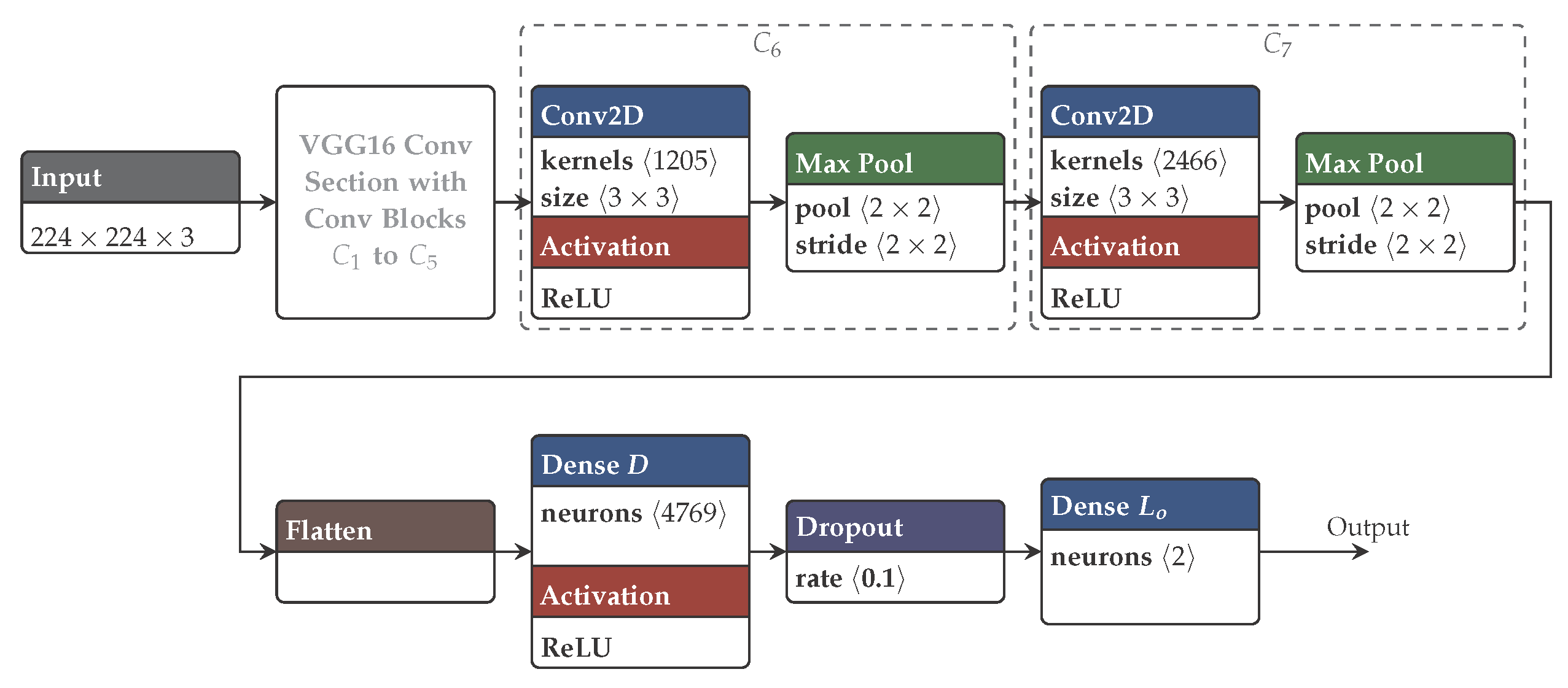
Figure 1. Diagram of Net FCD as example of the FCDN architecture.
Applsci 15 12779 g001
Figure 2. Samples from the outdoor dataset, depicting different 3D-printed models on differently coloured tablecloths and landscape. The entirety of usable images D is organised in further subgroups according to the depicted tablecloth surface (textured: D 0 x x ; uni-coloured: D 1 x x ), number of depicted objects (single: D x 0 x ; multiple: D x 1 x ) and object appearance (uni-coloured: D x x 0 ; textured: D x x 1 (Not available, as only a single textured object was available); mixed: D x x 2 ).
Applsci 15 12779 g002
Figure 3. Depiction of the computed southward oriented sun positions, which could be immediately used as label, if the device’s bearing B D , too, is pointing southwards (green). The azimuth label needs to be adjusted, if B D is pointing in a different direction (orange).
Applsci 15 12779 g003
Figure 4. Depictions of early, late and intermediate fusion with feature extraction stages (orange) and decision-making stages (blue) of a DNN. The data fusion element simply concatenates both data types in this study.
Applsci 15 12779 g004
Figure 5. Samples of the RGB data (left), depth data (centre) and normal data (right). Note: depth and normals are independent from the illumination, therefore no illumination-relevant information can be extracted from depth or normal information alone, which is why only an early fusion approach might benefit from this additional information.
Applsci 15 12779 g005
Figure 6. Box-and-whisker diagram of the angular estimation error distribution of Net s x , s y , LFAN, FCN, Net RTS and Net FCD . The median of the distribution is displayed as a green dashed line, the mean as red line and outliers as circular marks.
Applsci 15 12779 g006
Figure 7. Box-and-whisker diagrams depicting the angular estimation error distributions of the surface information experiments (colour coding as in Figure 6).
Applsci 15 12779 g007
Table 1. Subset split with number of contained images in parentheses.
Origin TestTraining/Validation
D 10 T D 10 (701) D S D 10 (1000)
D 100 T D 100 (195) D S D 100 (278)
D 101 T D 101 (506) D S D 101 (722)
D 11 T D 11 (200) D S D 11 (440)
D 110 T D 110 (80) D S D 110 (180)
D 112 T D 112 (120) D S D 112 (260)
Table 2. Prediction performance of the reference DNNs on T REAL .
e on T REAL Base Weights
Net s x , s y 7.1 ° ImageNet
LFAN 6.2 ° Net s x , s y
FCN 5.7 °
Net RTS 4.4 ° ImageNet
Net FCD 3.8 ° Net s x , s y
Table 3. Results on real outdoor data, depicting the prediction performance of unadapted DNNs in the upper and adapted DNNs in the lower section.
DNN T REAL S T D 0 T D 10 T D 11
Net s x , s y 7.1 ° 61.3 ° 63.5 ° 54.2 ° 45.9 °
Net RTS 4.4 ° 60.6 ° 41.5 ° 52.4 ° 44.4 °
Net FCD 3.8 ° 65.7 ° 47.5 ° 54.8 ° 49.2 °
Net DS D 10 33.3 ° 63.4 ° 48.2 ° 5.0 ° 36.3 °
Net DS REAL + DS D 10 7.0 ° 62.5 ° 41.4 ° 4.8 ° 36.1 °
Net DS REAL + DS D 10 / D 11 6.7 ° 61.8 ° 39.6 ° 5.8 ° 5.7 °
Table 4. Results of the trained strategies for RGB-D and RGB-N data with unmodified learning rate during fine-tuning and random initialization. Column T SDS contains the average angular error e and column p the p-value in relation to α = 0.01 .
T SDS Strategypr
Net base 0.9 ° n/an/an/a
RGB-D 0.9 ° S A < α 0.053
RGB-N 0.8 ° < α 0.167
RGB-D 0.7 ° S B < α 0.281
RGB-N 0.6 ° < α 0.461
Disclaimer/Publisher’s Note: The statements, opinions and data contained in all publications are solely those of the individual author(s) and contributor(s) and not of MDPI and/or the editor(s). MDPI and/or the editor(s) disclaim responsibility for any injury to people or property resulting from any ideas, methods, instructions or products referred to in the content.