Mechanical Properties and Degradation Mechanisms of Shallow Ili Loess Under Freezing and Thawing Conditions

Abstract

Existing freeze–thaw cycle tests are based on freeze–thaw cycles under fully constrained conditions, but under natural conditions, the vertical deformation of soil during freeze–thaw cycles is much greater than the lateral deformation. Therefore, to better simulate the freeze–thaw process of shallow soil under natural conditions, a method of preparing specimens is proposed. Specimens with five freeze–thaw cycle gradients, four water content gradients and three dry density gradients were prepared. This method realises the top-unconstrained role of the specimens during freeze–thaw cycles and provides space for vertical deformation. At the same time, it enables the observation of height and surface degradation. Triaxial tests of shallow Ili loess were carried out after indoor freeze–thaw cycles under fixed confining pressure (100 kPa). The results show that surface degradation and vertical deformation of Ili loess without top restraint increase gradually with the number of freeze–thaw cycles; strength decreases gradually and damage morphology changes from shear to bulging. Threshold conditions for the transition from softening to hardening in the strength curve of Ili shallow loess are proposed, as well as damage parameters related to freeze–thaw cycles, water content, and dry density. A coupled damage constitutive model applicable to shallow Ili loess has been established that takes these three factors into account.

1. Introduction

The Ili River Valley in Xinjiang, northwestern China, is an important seasonal frost zone with a unique and complex geological environment that poses a serious challenge to engineering construction [1]. Natural climatic factors, especially repeated freeze–thaw cycles, trigger strong engineering geological effects [2]. During the freezing period, the temperature gradient drives groundwater upwards, causing frost heaving of the surface loess and increasing the self-weight of the shallow soil while reducing its permeability [3]. During the snowmelt period, water cannot effectively seep down. On the other hand, it seeps down rapidly through permeability channels enlarged by freeze–thaw degradation. This causes the bottom loess to become significantly wetter and softer, and its strength decreases sharply. This can result in shallow loess landslides, roadbed bulging, pavement cracking, uneven settlement, frost heaving, and subsidence [1]. Therefore, when conducting engineering construction in the Ili region, especially for high-grade highways, railway roadbeds, slopes and foundation treatment, close attention must be paid to the impact of seasonal freeze–thaw cycles on shallow soil [4,5].

In studies of soil behaviour under freeze–thaw cycles, Ji et al. [6] observed that significant frost heaving forces develop during the freezing process. For shallow soils, these forces substantially exceed the overburden pressure, rendering their influence on soil behaviour non-negligible. Previous research is typically conducted under fully constrained conditions [7]. Shi et al. [8], Song et al. [9], and Yang et al. [10] find that in soils with low initial dry density, the dry density increases, whereas it decreases in soils with high initial dry density. This leads to a dual effect of either densification or loosening, depending on the initial dry density. After multiple freeze–thaw cycles, the dry density of the soil tends to converge to a specific value that depends only on the soil type. Ni et al. [11] and Xiao et al. [12], among others, reported that the particle size distribution of the soil changes after freeze–thaw cycles, with soil particles generally becoming smaller and more uniform. However, early studies on the shear strength of soil yield varied conclusions: some researchers argue that shear strength increases [13], others observe a decrease [14], and some report no significant change [15]. Lv et al. [16], Qi et al. [17], and others [18] noted that as the number of freeze–thaw cycles increase, the shape of the soil strength curve changes. Similarly, Fang et al. [19], Chang et al. [20], and others found that cohesion and the internal friction angle exhibit different trends after freeze–thaw cycles. Liu et al. [21] and others [22] demonstrated that the type of soil stress–strain curve is more influenced by water content than by freeze–thaw cycles. They also observe that water content differentially affects the degradation of failure strength under various freeze–thaw durations. Due to differences in test conditions, Su et al. [23] and Dong et al. [24] reported that soil strength and strength parameters gradually stabilised after about 10 freeze–thaw cycles, whereas Wang et al. [25] found that the soil reached a stable state after only seven cycles. Regarding the dynamic behaviour of soil under freeze–thaw cycles, Bai et al. [26] proposed that soil undergoes three stages: frost heaving, thaw settlement, and consolidation. These stages are influenced by temperature, the number of freeze–thaw cycles, and the duration of freeze–thaw periods. Wang et al. [27] found that saturated loess exhibits a stronger dynamic performance than non-freeze–thaw loess in a closed system without water replenishment; its structure also becomes more stable and denser. Liu et al. [28] noted that freeze–thaw cycles cause moisture redistribution in the soil, leading to increased strength in regions where moisture decreases and reduced strength in regions where moisture increases. Gao et al. [29] observed that soil particles fracture only at relatively coarse grain sizes, while fine particles tend to agglomerate due to the double electric layer effect. Clearly, the influence of freeze–thaw action on mechanical properties is essentially a process of continuous destruction and reorganisation of the soil’s internal structure [30]. From numerical simulations concerning boundary effects, it can be observed that optimising boundary conditions enables simulation results to more closely approximate experimental outcomes [31,32,33]. Therefore, to mitigate the influence of constraint forces during freeze–thaw cycles and to provide experimental data support for future numerical simulations, this study conducts a series of experiments that disregard the effect of top constraint during freeze–thaw cycles.

In summary, previous studies have primarily examined the impact of freeze–thaw cycles on soil in fully constrained environments. However, under natural conditions, freeze–thaw cycles cause relatively large vertical deformation and relatively small lateral deformation. When fully constrained soil is affected by frost heaving, the force generated causes the soil particles to be squeezed and broken, which leads to the degradation of the soil’s mechanical properties. Soil without top constraints undergoes vertical deformation, with the frost heaving force generated by freeze–thaw cycles being used partly to lift the soil and partly to squeeze the soil particles. Therefore, the degradation of the soil’s mechanical properties differs from that observed under fully constrained conditions. Studies on the mechanical properties of soil under freeze–thaw cycles should consider the effects of vertical deformation. Based on this, this paper presents a test method for investigating the mechanical properties of shallow Ili loess freeze–thaw soil with different dry densities and water contents. The method involves observing the surface degradation and height changes in the soil under freeze–thaw cycles. Threshold conditions for the transition from softening to hardening in the strength curve of freeze–thaw shallow Ili loess, as well as damage parameters related to freeze–thaw cycles, water content, and dry density, are proposed. A coupled damage constitutive model that meets the damage of shallow Ili loess and considers the three aforementioned factors was established.

2. Materials and Methods

2.1. Materials and Sample Preparation

2.1.1. Physical Properties of Loess

In this study, 2–3 m in situ soil samples were taken from the surface of the northwestern part of Shaha Village, Zeketai, Ili, Xinjiang, and the samples were taken by manual grooving, respectively, 150 mm × 150 mm × 150 mm cubic specimens and a number of loose soils were taken, and the samples were sealed with opaque adhesive tape and returned to the laboratory to be kept in a cool place after taking the samples. The in situ samples were measured according to GB/T 50123-2019 [34] Standard for Geotechnical Test Methods for their physical indexes (

Table 1. Physical parameters of the test soil.

Physical Properties	Value
Natural water content ($\omega /\%)$	3.00–6.00
Specific gravity of soil particles (Gs)	2.70
Natural density $({\rho }_0,\mathrm{g}/\mathrm{c}{\mathrm{m}}^3$)	1.43–1.48
Dry density $({\rho }_{\mathrm{d}},\mathrm{g}/\mathrm{c}{\mathrm{m}}^3)$	1.30–1.41
Initial porosity ratio (${\mathrm{e}}_0$)	0.96–1.02
Saturated water content (${\omega }_{\mathrm{r}}/\%$)	35.50
Plastic limit (${\omega }_{\mathrm{p}}/\%$)	19.16
Liquid limit (${\omega }_{\mathrm{L}}/\%$)	28.54
Plasticity index (${\mathrm{I}}_{\mathrm{P}}$)	9.38
Maximum dry density (${\rho }_{\mathrm{d}\mathrm{m}\mathrm{a}\mathrm{x}},\mathrm{g}/\mathrm{c}{\mathrm{m}}^3$)	1.79
Optimum water content (${\omega }_{\mathrm{o}\mathrm{p}}/\%$)	17.30
Soil category	CL

Ps: The classification of soils is determined based on the plasticity index ${\mathrm{I}}_{\mathrm{P}}$ and liquid limit ${\omega }_{\mathrm{L}}$. When plasticity index is greater than or equal to 7 and the liquid limit is less than 50, the soil is classified as a low-liquid-limit clay (i.e., CL).

) as well as particle gradation (Figure 1). After testing, the soil ${\mathrm{C}}_{\mathrm{c}}=0.32$, ${\mathrm{C}}_{\mathrm{u}}=6.90$ was poorly graded.

2.1.2. Sample Preparation

The test was configured according to the GB/T 50123-2019 [34] standard for geotechnical test methods for remodelled soil triaxial specimens. The naturally air-dried soil samples were crushed with a wooden mill, passed through a 2 mm sieve and placed in a sealed bag for storage. Soil samples with different water contents and dry densities were prepared indoors. The soil samples were sprayed to reach the target water content and then placed in a curing box for 24 h to allow the water to mix uniformly. A moisture content gradient and a dry density gradient were established based on the moisture content and dry density of the natural soil (i.e., undisturbed soil samples). Four water content gradients were set: 5.25%, 10.25%, 15.25% and 20.25%. Three dry density gradients were also set: 1.38 g/cm³, 1.43 g/cm³ and 1.48 g/cm³. The mass required to reach the expected dry density by compaction in layers under different water content was calculated.

Dynamic Compaction Sample Preparation [35], each layer was weighed at the same quality, divided into 5 layers with a diameter of 39.1 mm, 100 mm high transparent sample preparation apparatus was used for each layer of compaction, the surface was scraped to 2 mm deep and then the next layer was laid, until the height of the sample was 80 mm. Once the sample was made, the apparatus was covered with a latex film and tightened with a hoop. Finally, it was wrapped in a sealing bag to reduce water loss during freezing and thawing. To better observe soil height changes and surface degradation, saturated samples under three dry density conditions were added for freeze–thaw testing. The testing process is shown in Figure 2.

This sample preparation apparatus differs from previous devices, as illustrated in Figure 3. The apparatus comprises two sections: the lower section stands 80 mm high with an internal diameter of 39.1 mm, matching the specifications of conventional sample preparation devices. The upper section features a 20 mm high cap (hereafter referred to as the cap). This cap provides deformation space while simultaneously securing the lower section. During freeze–thaw cycle testing, the conventional apparatus constrained both ends, denying soil samples deformation space. Removing the upper constraints would compromise vertical deformation at the sample top, complicating comparative analysis. The new apparatus incorporates a cap, accommodating vertical soil deformation. This better reflects actual structural changes within shallow soils. Additionally, the apparatus’s transparency facilitates superior soil sample observation.

2.2. Experimental Method and Apparatus

2.2.1. Experimental Apparatus

An unconsolidated and undrained triaxial test was carried out using a TFB-1 strain-controlled unsaturated triaxial shear-permeability apparatus (Ningxi Soil Instrument Co., Ltd., Nanjing, China). A freeze–thaw cycle test was carried out using a TDS-300 freeze–thaw tester (Donghua Testing Instruments Co., Ltd., Suzhou, China). Soil maintenance was carried out using a SHBY-40B standard constant-temperature and constant-humidity curing box (China Hebei Dahong Laboratory Instruments Co., Ltd., Cangzhou, China). A vacuum pumping saturator was used to saturate the soil samples. The freezing and thawing box used cold-conducting liquid for cooling and had a fan installed in the upper part of the box to simulate strong weathering. When the temperature rose, the water inlet pump released water and the liquid level in the box rose to a certain height. The temperature of the liquid controlled the temperature of the entire box; the freezing and thawing box had no temperature gradient or replenishment of water. The test apparatus is shown in Figure 4 below.

2.2.2. Freezing-Thawing Test

The moulds containing the soil samples were sealed and placed in the freezing and thawing box. Five kilograms of discus were placed on top to ensure the samples were vertical and the mould parts were in close contact to minimise water loss. No water replenishment occurred during the freeze–thaw process. According to local meteorological data for Ili, the freezing temperature was set to −20 °C and the thawing temperature to 20 °C. The box temperature reduction took 30 min, followed by 11 h of constant temperature freezing. The box temperature increase took 30 min, followed by 11 h of constant temperature melting. After testing, the soil samples could be completely frozen and melted. One cycle took 24 h (Figure 5). The cycle number was set to 0, 1, 3, 7 or 11 times, for a total of five groups of tests. Each group contained one fixed water content, three kinds of dry density, and five kinds of cycle times, for a total of 75 specimens. The specimens were fully saturated using a vacuum pumping saturation device for at least 4 h, followed by water immersion for at least 10 h to ensure full saturation. Before saturation, the mould containing the soil samples was placed in the device. Filter paper and permeable stone were placed on the upper and lower surfaces of the soil samples. The entire mould was then wrapped in a latex membrane and a 5 kg iron cake was placed on top to ensure the membrane was tightly connected and prevent soil loss. Following completion of the freeze–thaw cycles, the samples were weighed, revealing their mass to be essentially unchanged from prior to the cycles. The average height variation in the soil samples was recorded by taking measurements at four points on their upper surface. Triaxial tests were then conducted immediately thereafter to prevent interference from other factors.

2.2.3. Triaxial Shear Test

After the freeze–thaw cycles, an unconsolidated and undrained triaxial shear test was carried out under a confining pressure of 100 kPa using a TFB-1 type of strain-controlled unsaturated triaxial shear-permeability. Due to changes in the height of the specimens at the end of the freeze–thaw cycles, the height parameters needed to be adjusted at the start of the experiment. According to the standard for geotechnical engineering test methods (GB/T 50123-2019 [34]), the shear rate was set to 0.8 mm/min and the test was terminated when the axial strain reached 20%. Stress–strain curves were obtained for different dry densities and water contents under the action of the freeze–thaw cycles, as well as damage patterns of the specimens. The test programme is shown in

Table 2. Experimental programme.

Test Number	Water Content ω (%)	$\mathbf{Dry} \mathbf{Density} {\mathbf{\rho }}_{\mathbf{d}}$ (g/cm3)	Freeze–Thaw Times (times)	Confining Pressure σ3 (kPa)
1	5.25	1.38, 1.43, 1.48	0, 1, 3, 7, 11	100
2	10.25	1.38, 1.43, 1.48	0, 1, 3, 7, 11	100
3	15.25	1.38, 1.43, 1.48	0, 1, 3, 7, 11	100
4	20.25	1.38, 1.43, 1.48	0, 1, 3, 7, 11	100
5	Saturated	1.38, 1.43, 1.48	0, 1, 3, 7, 11

.

3. Experimental Results and Analysis

3.1. Results of the Triaxial Test

3.1.1. Effect of Initial Water Content and Dry Density

To investigate the influence of initial water content and dry density on the mechanical properties of shallow Ili loess under confining pressure, specimens were tested under 100 kPa confining pressure. Stress–strain curves and damage patterns were analysed for soils with varying water contents and dry densities. By comparing with the relevant literature featuring similar water content and dry density [16,22,36], similar conclusions were drawn. The greater the dry density of the soil, the higher its strength; conversely, the greater the water content, the lower the strength. The peak strain point on the softening curve typically occurs within the 3–6% strain range. When exceeding specific water content or dry density thresholds, the stress–strain curve type of the soil undergoes transformation. The distinction lies in the differing critical values for the transition of curve type (from strain softening to strain hardening) and failure mode (from shear failure to swelling failure), with this study identifying 15.25% as the threshold. As shown in Figure 6, $\omega$ represents the water content, ${\rho }_{\mathrm{d}}$ represents the dry density, $\mathrm{N}$ represents the number of freezing and thawing cycles, and ${\sigma }_3$ represents the confining pressure. As can be seen in Figure 6a,b, when the confining pressure is 100 kPa and the water content is low (5.25% or 10.25%), the stress–strain curve of the unfrozen–thawed soil exhibits softening, the peak strength increases with increasing dry density and the peak point shifts towards strain reduction with increasing dry density. After the soil body reaches peak strength, the strength decreases at a faster rate due to the emergence of shear surfaces (sliding zones) and then stabilises. The residual strength of the soil body increases with dry density, and the damage pattern is shear damage. As can be seen in Figure 6c,d, the stress–strain curves are of the hardening type at the higher water contents of 15.25% and 20.25%. The destructive strength and elastic modulus of the soil body increase with dry density, and the demarcation point between the elastic and plastic segments shifts towards strain reduction. The soil body gradually compacts under load and does not reach ultimate strength; at this stage, the damage pattern is bulging. As can be seen from Figure 7a–c, the soil’s stress–strain curve changes from a strain-softening type to a strain-hardening type as the water content increases. The peak strength and elastic modulus decrease as the initial water content increases. This transition in stress–strain curve type occurs at the stage of transition between lower and higher water content (i.e., 10.25% to 15.25%, Reference [22] ranges from 10% to 18%), when the soil’s strength degrades the most. This suggests that a critical water content value (near the optimum water content) exists for the transition from strain softening to strain hardening and causing the effect of water content on strength to increase significantly. It indicates that a threshold water content exists (near the optimum water content) at which strain softening transitions to strain hardening, causing a surge in the effect of water content on strength. The compaction characteristics of the soil body show that, as the water content increases, the maximum dry density value first increases and then decreases. The soil body in the vicinity of the optimum water content corresponds to a higher maximum dry density value and a greater discrepancy with the test set value. At this point, the soil is looser, so its strength decreases more obviously at this water content. As can be seen from the stress–strain curve, the deformation is mainly divided into three stages [37]:

(1)

Elastic deformation stage: During this process, the deviatoric stress increases linearly with the increase in axial strain, resulting in recoverable elastic deformation. An increase in the number of freeze–thaw cycles reduce the elastic modulus of the sample.

(2)

Elastic-plastic deformation stage: During this stage, the relationship between deviatoric stress and axial strain becomes nonlinear. At this stage, damage has already occurred within the sample and small pores and cracks are beginning to form, but the soil particle skeleton can still bear some of the load.

(3)

At low water content, the pores and cracks inside the sample connect. The sample loses its bearing capacity at this point, its strength decreases rapidly, shear failure occurs and a clear shear surface appears on the sample. At high water content, the sample fails due to bulging and no shear surface appears.

The failure mode of the soil is analysed based on Figure 8. At low water content, when the dry density is 1.38 g/cm³, a clear shear surface is formed when the soil fails; when the dry density is 1.43 g/cm³ and 1.48 g/cm³, two intersecting shear surfaces are formed when the soil fails. It can be seen that as the dry density increases, there is a tendency for multiple shear surfaces to form on the surface of the sample, and the shear surfaces formed become more and more significant. The test results are similar to those reported in References [16,31], but due to differences in soil samples, the range of dry density corresponding to changes in the number of shear planes varies. The higher the dry density of the soil, the more compact and stable its internal skeleton is, and the greater its stiffness. Therefore, when subjected to a load, multiple shear planes are formed. The appearance of shear planes is reflected in a phase of rapid strength decline in the stress–strain diagram, which is consistent with the test results. The higher the water content, the lower the soil stiffness. Therefore, at high water contents of 15.25% and 20.25%, the soil undergoes bulging failure (The experimental results are similar to those reported in reference [36]. This paper summarises the extent of bulging deformation.), with the degree of bulging becoming more significant as the dry density increases. At a constant dry density, the soil’s failure mode changes from shear to bulging as the water content increases.

3.1.2. Effects of Freezing and Thawing Under Wet-Dense Conditions

To investigate the effects of freeze–thaw cycles on shallow loess in Ili, thawed specimens were tested under 100 kPa confining pressure, with analysis conducted on their stress–strain curves and damage morphology. Prior to testing, adjustments to the height parameter within the triaxial apparatus were required due to changes in the height of the soil samples. As the same phenomenon occurred in soils with certain water contents, soils with water contents of 10.25% and 20.25% were selected for analysis. As Figure 9a–c show, at a water content of 10.25%, the stress–strain curve of soil with a dry density of 1.38 g/cm³ changed from softening to hardening after one freeze–thaw cycle. After seven cycles, the curve for a dry density of 1.43 g/cm³ changed from softening to hardening; after 11 cycles, the curve for a dry density of 1.48 g/cm³ remained softening. As the number of freeze–thaw cycles increases, the elastic modulus and peak strength of the soil decrease gradually, and the peak point of the strain softening curve shifts towards higher strains [36]. After seven cycles, the strength stabilises. Freeze–thaw action destroys the cementation and skeletal structure within the soil [38]. Frost heaving causes the larger particles within the soil to break, thereby increasing the number of pores and loosening the soil. As dry density increases, soil cementation strengthens, the skeleton becomes more stable and frost resistance improves [3,11,16]. Consequently, more freeze–thaw cycle times are required for the stress–strain curve to change from softening to hardening. Figure 9d–f show that, when the water content is 20.25%, the elastic modulus and peak strength of soil with a dry density of 1.38 g/cm³ continue to increase with freeze–thaw cycles times. For soil with dry densities of 1.43 g/cm³ and 1.48 g/cm³, there was an initial increase followed by a decrease. Following freeze–thaw cycles, the elastic modulus and strength of the soil increased, with the strength stabilising after three cycles. This demonstrates that, in the absence of top constraints, soil undergoes cementation or consolidation in addition to frost heaving damage under freeze–thaw conditions [26]. At low water content, frost heaving has a greater effect on the soil, decreasing its strength. However, at high water content, consolidation or cementation has a greater effect, increasing its strength slightly. Soil with a low dry density undergoes freeze–thaw cycles, becoming denser and gradually gaining strength. Once a certain density is reached; however, frost heaving occurs again, reducing the strength [27,39]. Soil with high dry density experiences more obvious frost heaving at a certain water content, and its strength is reduced by the force of frost heaving [24]. Subsequently, the strengthening effect of consolidation or cementation on the soil gradually increases with the number of freeze–thaw cycles, creating a new equilibrium.

3.2. Patterns of Change in Peak Intensity and Height of Soil Samples

3.2.1. Effect of Freeze–Thaw Action on Peak Strength Under Wet–Dense Conditions

Peak strength reflects the bearing capacity of soil under load. In order to study the effects of freeze–thaw cycles on shallow Ili loess, we analysed the changes in peak strength in order to quantify the degree of damage caused to the soil by freeze–thaw cycles under wet–dense conditions.

As shown in Figure 10, the peak strength of the soil decreases with an increase in the number of freeze–thaw cycles when the water content is 5.25%, 10.25%, and 15.25% under three dry densities. The peak strength of the soil at three dry densities degrades the most when the water content is 10.25%, decreasing by 24.14%, 14.21%, and 17.91% with an increase in the number of freeze–thaw cycles. This is because, when the water content is 5.25%, the water content in the soil is low and the effect of frost heaving is small, resulting in less strength degradation [40,41]. Conversely, when the water content is 15.25%, the frost heaving effect is significant, yet the initial strength is low, also leading to less strength degradation. When the water content is 20.25% and the dry density is 1.38 g/cm³, the soil strength increases gradually with the number of freeze–thaw cycles, rising by 7.53%, 4.15%, 2.81% and 2.87%, respectively, stabilising after seven cycles. However, when the dry density is 1.43 or 1.48 g/cm³, the soil strength first increases and then decreases with the number of freeze–thaw cycles, and the number of cycles required to reach a stable strength increases [42]. The peak strength of the soil increases as dry density increases. When the water content was 5.25% and there were 0 or 1 freeze–thaw cycles, the soil strength increased by 45.98% or 43.11%, respectively, with an increasing dry density. When the water content was 10.25% and there were three, seven, and eleven freeze–thaw cycles, the strength increased by 39.56%, 44.14%, and 44.21%, respectively, with an increasing dry density. Without freeze–thaw cycles and with a water content of 5.25%, the soil’s strength increased the most with dry density. This indicates that the initial dry density had a greater effect on peak strength than the freeze–thaw cycles. The peak strength of the soil decreased with increasing water content. When the water content increased from 10.25% to 15.25%, the strength decreased by around 50% at all dry densities and freeze–thaw cycles.

In order to better illustrate the threshold conditions for the transition from softening to hardening of the curves, the peak intensities are normalised as in the following Equation (1), the k value represents the ratio of the difference between the peak intensity of the test sample and the minimum peak intensity among all samples to the difference between the maximum and minimum peak intensities among all samples:

$$\mathrm{K}={\displaystyle \frac{\left(\sigma -{\sigma }_{\mathrm{m}\mathrm{i}\mathrm{n}}\right)}{\left({\sigma }_{\mathrm{m}\mathrm{a}\mathrm{x}}-{\sigma }_{\mathrm{m}\mathrm{i}\mathrm{n}}\right)}}$$

(1)

where $\mathrm{K}$ is the normalised peak intensity; $\sigma$ is the peak intensity of the soil sample; ${\sigma }_{\mathrm{m}\mathrm{a}\mathrm{x}}$ and ${\sigma }_{\mathrm{m}\mathrm{i}\mathrm{n}}$ are the minimum and maximum values of the peak intensity in all soil samples, respectively. The normalised peak intensities are summarised according to the above equation in

Table 3. Normalised peak intensities.

	$\mathbf{N}$ (Times)	0	1	3	5	7
${\mathbf{\rho }}_{\mathbf{d}} \mathbf{(}\mathbf{g}\mathbf{/}{\mathbf{cm}}^{\mathbf{3}}\mathbf{)}\mathbf{/}\mathbf{\omega } \mathbf{(}\mathbf{\%}\mathbf{)}$		$\mathbf{K}$
1.38/5.25		0.597	0.529	0.524	0.513	0.462
1.38/10.25		0.532	0.475	0.427	0.366	0.337
1.38/15.25		0.105	0.102	0.075	0.078	0.073
1.38/20.25		0.000	0.020	0.033	0.042	0.051
1.43/5.25		0.741	0.727	0.723	0.696	0.655
1.43/10.25		0.631	0.607	0.575	0.523	0.502
1.43/15.25		0.165	0.147	0.130	0.118	0.107
1.43/20.25		0.021	0.045	0.081	0.047	0.046
1.48/5.25		1.000	0.876	0.808	0.783	0.700
1.48/10.25		0.802	0.745	0.705	0.651	0.608
1.48/15.25		0.258	0.209	0.195	0.192	0.177
1.48/20.25		0.067	0.113	0.136	0.150	0.124

, Figure 11 below.

In summary, the normalised peak strength of K = 0.5 is defined as the conversion threshold of the curve. When K > 0.5, the soil strength curve is of the softening type, and when K < 0.5, it is of the hardening type. For shallow Ili loess, strength decreases gradually with the number of freeze–thaw cycles at different water contents. When the water content exceeds the plastic limit, the soil strength after the freeze–thaw cycles is higher than it would be without them. At this water content, the strength of soil with a low dry density increases with the number of freeze–thaw cycles. As dry density increases, soil strength initially increases and then decreases with the number of freeze–thaw cycles. The greater the initial water content of shallow Ili loess, the greater the effect of the freeze–thaw cycles. The greater the initial dry density, the more the freeze–thaw cycles are required to reach stable strength. Reference [43] indicates that water content exerts a greater influence on soil properties than dry density. This study analyses the reduction in peak strength of soil under freeze–thaw cycling conditions and finds that water content has a more pronounced effect on soil strength than dry density, while dry density itself exerts a greater influence than the number of freeze–thaw cycles.

3.2.2. Impact of Freeze–Thaw Cycles on Height and Damage Patterns

To study the effect of freeze–thaw cycles on shallow Ili loess height, changes in sample height and surface degradation were recorded. $\Delta h$ (mm) denotes the height increase in the soil sample under freeze–thaw cycles.

As can be seen in Figure 12, soil height increases with dry density, first rising and then falling with increasing water content, before stabilising after three freeze–thaw cycles. This is because, at the same water content, greater dry density results in closer contact between soil particles, greater stiffness of the soil, fewer internal pores and a smaller effect of frost heaving on the displacement and rearrangement of soil particles [30]. As the water content increased from 10.25% to 15.25%, the height of the soil sample decreased. Due to the high water content, the shallow Ili loess was greatly affected by freezing and thawing at this point, becoming loose, less rigid, and more plastic with larger internal pores [44]. The force of frost heaving caused the soil particles to shift and rearrange, thereby filling the pores [45]. The height only changed after the soil had gradually compacted, so there was a slight decrease in height [46].

As the height change in the unsaturated sample was not obvious, this may have caused errors in the test. The following is an analysis of the saturated sample (=100%). Due to uneven height changes in the soil during frost heaving, thaw settlement and consolidation, height changes were recorded using the four-point average method. As can be seen in Figure 13, the soil’s height change increases with dry density and first increases, then decreases with an increase in freeze–thaw cycles. Soil at all dry densities exhibited a height variation trend that initially increased then decreased following the 7 freeze–thaw cycles before. After seven freeze–thaw cycles, soil with a dry density of 1.48 g/cm³ showed a slight increase in height variation, though this was significantly less pronounced than the height changes induced by the initial seven cycles. Soils with dry densities of 1.38 and 1.43 g/cm³ exhibited a trend of continuous height reduction until stabilisation. Consequently, soils with a higher dry density require a greater number of freeze–thaw cycles to achieve a stable state. As can be seen from the figure, if the top of the soil is unconstrained, it will always be in dynamic equilibrium under the influence of freezing and thawing (i.e., frost heaving will dominate first, followed by thaw settlement, alternating back and forth [29]), eventually stabilising. The greater the dry density of the soil, the more times it will reach a stable state of freezing and thawing. Previous studies have shown that the initial frost heaving water content is roughly equal to the plastic limit water content of the soil [47]. At saturated water content, the soil has highly water content, and during the freeze–thaw cycles process, moisture migration easily forms a freezing front [48]. This leads to a significant increase in vertical volume. Soils with a low water content find it difficult to form a frozen surface and generally undergo in situ freezing, so the volume change is not obvious. This shows that, when the soil’s water content reaches a certain level, its dry density increases and the contact area between soil particles and ice crystals during the freezing process also increases. This has a greater effect on frost heaving, resulting in greater changes in height [49].

The saturated samples had a high free water content and were damaged by water migration during freeze–thaw cycles, which affected their internal structure. As can be seen in Figure 14, the height of the samples increased unevenly at all three dry densities after undergoing the first and third freeze–thaw cycles. Debris from soil particles and cracks appeared on the surface of the specimens. As the dry density increased, the amount of debris and cracks gradually decreased. Freeze–thaw cycles had a greater impact on the upper part of the soil than the lower part, and the scope of the impact gradually decreased as the dry density increased. Thaw settlement occurred in all three types of soil with different dry densities when the number of freeze–thaw cycles reached seven, and the height of the soil samples decreased. After 11 cycles, the soil with a dry density of 1.48 g/cm³ exhibited frost heaving, while the other two densities showed thaw settlement. After undergoing seven and 11 freeze–thaw cycles, the debris and cracks on the soil surface gradually increased in number and spread from the upper part to the lower part of the soil sample, eventually covering the entire sample.

In summary, in the initial freeze–thaw stage (N = 1, 3), greater dry density results in shallow Ili loess less degradation of the upper soil surface in a saturated state. However, with an increase in the number of freeze–thaw cycles (N = 7, 11), greater surface degradation occurred at higher dry densities. At three dry densities, increasing surface degradation occurred with an increased number of freeze–thaw cycles. This is because higher dry soil density increases frost resistance, reducing damage in the early stages of freeze–thaw. Once the threshold is reached (between three and seven times in this study), the contact area between the soil’s internal particles and ice crystals increases in soils with a high dry density. This causes frost heaving to rapidly destroy the soil structure, resulting in an intensification of surface degradation as dry density increases [49]. This demonstrates that, when shallow Ili loess reaches a certain water content, different phenomena occur at different dry densities due to the influence of freeze–thaw cycles. Under saturated conditions, shallow Ili loess alternates between frost heaving and thaw settlement during freeze–thaw cycles before reaching a stable state. The higher the dry density, the more freeze–thaw cycles are required to reach this state of stability [50].

4. Establishment and Parameterization of the Intrinsic Model

A constitutive model of soil is a mathematical model that describes macroscopic mechanical properties. Based on the Binary-Medium Model [51,52], this paper examines how the strength and deformation characteristics of Ili loess are affected by the number of freeze–thaw cycles, water content and dry density, in the absence of top constraints. It then establishes a constitutive model under the influence of these three factors.

4.1. Model Building

The model is based on triaxial tests. The Binary-Medium Model assumes that, during the loading process, the soil is supported by two parts: bonded blocks and weakened bands. Initially, the load is primarily supported by the bonded blocks and the stress–strain relationship satisfies Hooke’s law. As loading continues, weakened bands gradually form and plastic deformation occurs within the soil. Even after complete destruction, the soil sample retains a certain bearing capacity, i.e., residual stress.

It is known from the principle of strain equivalence [53] (as shown in Equation (2)), ${\sigma }^{\prime }$ denotes effective stress, ${\epsilon }^{\prime }$ denotes effective strain, which can be determined from the stress–strain curve. D denotes the total damage factor, which may be calculated according to the following Equation (3):

$${\sigma }^{\prime } = \mathrm{E}{\epsilon }^{\prime }(1-\mathrm{D})$$

(2)

where ${\sigma }^{\prime }$ is the effective stress; $\mathrm{E}$ is the modulus of elasticity of the bonded blocks; ${\epsilon }^{\prime }$ is the effective strain; and $\mathrm{D}$ is the damage factor.

The damage of the soil body consists of two parts: initial damage and load loading, so the damage factor $\mathrm{D}$ is selected by using a coupled damage evolution, i.e.,:

$$\mathrm{D}={\mathrm{D}}_0+{\mathrm{D}}_{\mathrm{L}}-{\mathrm{D}}_0{\mathrm{D}}_{\mathrm{L}}$$

(3)

where ${\mathrm{D}}_0$ is the initial damage; ${\mathrm{D}}_{\mathrm{L}}$ is the damage caused by load action; ${\mathrm{D}}_0{\mathrm{D}}_{\mathrm{L}}$ is the damage caused by coupling action.

Since the damage of bonded blocks satisfies the elastic theory, the change in elastic modulus is used as the damage factor. Since water content causes soil strength reduction and freeze–thaw cycles also cause strength reduction, the coupled damage ${\mathrm{D}}_0$ of freeze–thaw cycles and water content is defined in terms of elastic modulus, respectively. In order to facilitate the subsequent writing, ${\displaystyle \frac{{\mathrm{E}}_{\mathrm{n}}}{{\mathrm{E}}_0}}$ is defined as the freeze–thaw degradation factor. $\alpha$ is defined as the ratio of the elastic modulus after a freeze–thaw cycle to the reference modulus (without freeze–thaw); ${\displaystyle \frac{{\mathrm{E}}_{\omega }}{{\mathrm{E}}_{\omega 0}}}$ is defined as the water content degradation factor. β denotes the ratio of the elastic modulus of a specimen at a certain water content to its elastic modulus at the initial water content.; and ${\displaystyle \frac{{\mathrm{E}}_{\rho }}{{\mathrm{E}}_{\rho 0}}}$ is defined as the dry density degradation factor. $\gamma$ denotes the ratio of the elastic modulus of a specimen at a given dry density to the elastic modulus at the maximum dry density of experimental setup, as follows:

$${\mathrm{D}}_{\mathrm{N}}=1-{\displaystyle \frac{{\mathrm{E}}_{\mathrm{n}}}{{\mathrm{E}}_0}}=1-\alpha$$

(4)

$${\mathrm{D}}_{\omega }=1-{\displaystyle \frac{{\mathrm{E}}_{\omega }}{{\mathrm{E}}_{\omega 0}}}=1-\beta$$

(5)

Then the coupled damage of freeze–thaw and water content can be expressed as:

$${\mathrm{D}}_0={\mathrm{D}}_{\mathrm{N}}+{\mathrm{D}}_{\omega }-{\mathrm{D}}_{\mathrm{N}}{\mathrm{D}}_{\omega }$$

(6)

$${\mathrm{D}}_0=1-{\displaystyle \frac{{\mathrm{E}}_{\mathrm{n}}{\mathrm{E}}_{\omega }}{{\mathrm{E}}_0{\mathrm{E}}_{\omega 0}}}=1-\alpha \beta$$

(7)

where ${\mathrm{E}}_{\mathrm{n}}$ is the resilient modulus of soil after $\mathrm{N}$ freeze–thaw cycles; ${\mathrm{E}}_0$ is the resilient modulus of soil without freeze–thaw cycles; ${\mathrm{E}}_{\omega }$ is the resilient modulus of soil corresponding to the water content at which the test was carried out; and ${\mathrm{E}}_{\omega 0}$ is the resilient modulus of soil corresponding to the initial value of water content at which the test was set.

Since the reduction in dry density also reduces the strength of the soil, the modulus of elasticity is still used to define the strength degradation caused by the reduction in dry density:

$${\mathrm{D}}_{\rho }=1-{\displaystyle \frac{{\mathrm{E}}_{\rho }}{{\mathrm{E}}_{\rho 0}}}=1-\gamma$$

(8)

where ${\mathrm{E}}_{\rho }$ is the modulus of elasticity corresponding to the dry density at which the test was conducted; ${\mathrm{E}}_{\rho 0}$ is the modulus of elasticity corresponding to the dry density at which the test was set to maximum.

At this point, from the aforementioned Equations (7) and (8), the initial damage under three factors is derived through the coupling damage process. As shown in Equation (9):

$${\mathrm{D}}_0=1-{\displaystyle \frac{{\mathrm{E}}_{\mathrm{n}}{\mathrm{E}}_{\omega }{\mathrm{E}}_{\rho }}{{\mathrm{E}}_0{\mathrm{E}}_{\omega 0}{\mathrm{E}}_{\rho 0}}}=1-\alpha \beta \gamma$$

(9)

When there is only one dry density and water content, the equation degenerates to:

$${\mathrm{D}}_0={\mathrm{D}}_{\mathrm{N}}=1-{\displaystyle \frac{{\mathrm{E}}_{\mathrm{n}}}{{\mathrm{E}}_0}}=1-\alpha$$

(10)

Damage under loading consists of damaged particles and undamaged particles. Therefore, the damage factor of loess under loading can be expressed as the ratio of the number of damaged microelements to the total number of microelements:

$${\mathrm{D}}_{\mathrm{L}}={\displaystyle \frac{{\mathrm{S}}_{\mathrm{f}}}{\mathrm{S}}}$$

(11)

where ${\mathrm{S}}_{\mathrm{f}}$ is the number of damaged microelements inside the soil; $\mathrm{S}$ is the total number of soil microelements.

The introduction of randomly distributed composite functions [54] quantitatively describes the intensity of microelements:

$$\mathrm{f}\left(\epsilon \right)={\displaystyle \frac{5\frac{\mathrm{m}}{{\epsilon }_0}{\left(\frac{\epsilon }{{\epsilon }_0}\right)}^{\mathrm{m}-1}}{{\left[1+{\left(\frac{\epsilon }{{\epsilon }_0}\right)}^{\mathrm{m}}\right]}^6}}$$

(12)

where $\epsilon$ is the strain of the soil; $\mathrm{m}$ and ${\epsilon }_0$ are the parameters of the distribution of the composite function related to the mechanical properties of the soil.

Then the number of microelements damaged in the soil as a whole is:

$${\mathrm{S}}_{\mathrm{f}}={\int }_0^{\epsilon } \mathrm{S}\mathrm{f}\left(\epsilon \right)\mathrm{d}\epsilon =\mathrm{S}\left\{\mathrm{C}-{\displaystyle \frac{1}{{\left[1+{\left(\frac{\epsilon }{{\epsilon }_0}\right)}^{\mathrm{m}}\right]}^5}}\right\}$$

(13)

where $\mathrm{C}$ is a constant. The damage factor of loess under loading is obtained by bringing in Equation (11):

$${\mathrm{D}}_{\mathrm{L}}={\int }_0^{\epsilon } \mathrm{f}\left(\epsilon \right)\mathrm{d}\epsilon =\left\{\mathrm{C}-{\displaystyle \frac{1}{{\left[1+{\left(\frac{\epsilon }{{\epsilon }_0}\right)}^{\mathrm{m}}\right]}^5}}\right\}$$

(14)

When the soil is not damaged, $\epsilon =0$, $\mathrm{D}=0$, which gives $\mathrm{C}=1$, which can be obtained by combining the above Equations (2), (3), (9) and (14):

$$\mathrm{D}=1-{\displaystyle \frac{\alpha \beta \gamma }{{\left[1+{\left(\frac{{\epsilon }_1^{\prime }}{{\epsilon }_0}\right)}^{\mathrm{m}}\right]}^5}}$$

(15)

$${\sigma }_1-{\sigma }_3=\mathrm{E}{\epsilon }_1^{\prime }\left(1-\mathrm{D}\right)$$

(16)

where ${\sigma }_1-{\sigma }_3$ are the deviatoric stresses of the loess microelement; ${\epsilon }_1^{\prime }$ is the axial effective strain of the loess.

When there is only one water content and dry density degree, the total damage equation degenerates to:

$$\mathrm{D}=1-{\displaystyle \frac{{\mathrm{E}}_{\mathrm{n}}}{{\mathrm{E}}_0{\left[1+{\left(\frac{{\epsilon }_1^{\prime }}{{\epsilon }_0}\right)}^{\mathrm{m}}\right]}^5}}=1-{\displaystyle \frac{\alpha }{{\left[1+{\left(\frac{{\epsilon }_1^{\prime }}{{\epsilon }_0}\right)}^{\mathrm{m}}\right]}^5}}$$

(17)

when the soil is completely destroyed ($\mathrm{D}=1$), the soil still has a certain bearing capacity and this part is the residual shear strength. Therefore, the deviatoric stress of loess is borne by two parts, which can be expressed as:

$${\sigma }_1-{\sigma }_3=({\sigma }_1-{\sigma }_3{)}_{\mathrm{D}}+({\sigma }_1-{\sigma }_3{)}_{\mathrm{F}}$$

(18)

$$({\sigma }_1-{\sigma }_3{)}_{\mathrm{D}}={\mathrm{D}\left({\sigma }_1-{\sigma }_3\right)}_{\mathrm{r}}$$

(19)

$$({\sigma }_1-{\sigma }_3{)}_{\mathrm{F}}=\mathrm{E}{\epsilon }_1^{\prime }(1-\mathrm{D})$$

(20)

where ${\sigma }_1-{\sigma }_3$ is the deviatoric stress borne by the microelement of the damaged part of the soil; ${\left({\sigma }_1-{\sigma }_3\right)}_{\mathrm{r}}$ is the residual deviatoric stress; and $({\sigma }_1-{\sigma }_3{)}_{\mathrm{F}}$ is the deviatoric stress borne by the undamaged part of the soil. Equation (15) is brought into Equations (19) and (20). From the principle of strain equivalence, the effective variable of loess is equal to the apparent strain [55,56], i.e., $\epsilon ={\epsilon }_1^{\prime }$. In summary, the damage statistical model of loess is:

$${\sigma }_1-{\sigma }_3={\displaystyle \frac{{\mathrm{E}}_{\mathrm{n}}{\mathrm{E}}_{\omega }{\mathrm{E}}_{\rho }{\epsilon }_1^{\prime }}{{\mathrm{E}}_{\omega 0}{\mathrm{E}}_{\rho 0}{\left[1+{\left(\frac{{\epsilon }_1^{\prime }}{{\epsilon }_0}\right)}^{\mathrm{m}}\right]}^5}}+{\left({\sigma }_1-{\sigma }_3\right)}_{\mathrm{r}}\left\{1-{\displaystyle \frac{{\mathrm{E}}_{\mathrm{n}}{\mathrm{E}}_{\omega }{\mathrm{E}}_{\rho }}{{\mathrm{E}}_0{\mathrm{E}}_{\omega 0}{\mathrm{E}}_{\rho 0}{\left[1+{\left(\frac{{\epsilon }_1^{\prime }}{{\epsilon }_0}\right)}^{\mathrm{m}}\right]}^5}}\right\}$$

(21)

i.e.,

$${\sigma }_1-{\sigma }_3={\displaystyle \frac{\beta \gamma {\mathrm{E}}_{\mathrm{n}}{\epsilon }_1^{\prime }}{{\left[1+{\left(\frac{{\epsilon }_1^{\prime }}{{\epsilon }_0}\right)}^{\mathrm{m}}\right]}^5}}+{\left({\sigma }_1-{\sigma }_3\right)}_{\mathrm{r}}\left\{1-{\displaystyle \frac{\alpha \beta \gamma }{{\left[1+{\left(\frac{{\epsilon }_1^{\prime }}{{\epsilon }_0}\right)}^{\mathrm{m}}\right]}^5}}\right\}$$

(22)

The constitutive model degenerates when there is only one dry density and dry density:

$$\begin{gathered} {\sigma }_1-{\sigma }_3={\displaystyle \frac{{\mathrm{E}}_{\mathrm{n}}{\epsilon }_1^{\prime }}{{\left[1+{\left(\frac{{\epsilon }_1^{\prime }}{{\epsilon }_0}\right)}^{\mathrm{m}}\right]}^5}}+{\left({\sigma }_1-{\sigma }_3\right)}_{\mathrm{r}}\left\{1-{\displaystyle \frac{{\mathrm{E}}_{\mathrm{n}}}{{\mathrm{E}}_0{\left[1+{\left(\frac{{\epsilon }_1^{\prime }}{{\epsilon }_0}\right)}^{\mathrm{m}}\right]}^5}}\right\} \\ ={\displaystyle \frac{{\mathrm{E}}_{\mathrm{n}}{\epsilon }_1^{\prime }}{{\left[1+{\left(\frac{{\epsilon }_1^{\prime }}{{\epsilon }_0}\right)}^{\mathrm{m}}\right]}^5}}+{\left({\sigma }_1-{\sigma }_3\right)}_{\mathrm{r}}\left\{1-{\displaystyle \frac{\alpha }{{\left[1+{\left(\frac{{\epsilon }_1^{\prime }}{{\epsilon }_0}\right)}^{\mathrm{m}}\right]}^5}}\right\} \end{gathered}$$

(23)

The model contains seven parameters, ${\mathrm{E}}_{\mathrm{n}},\mathrm{m},{\epsilon }_0,\alpha ,\beta ,\gamma ,{\left({\sigma }_1-{\sigma }_3\right)}_{\mathrm{r}}$. Among them, ${\mathrm{E}}_{\mathrm{n}},\alpha ,\beta ,\gamma ,{\left({\sigma }_1-{\sigma }_3\right)}_{\mathrm{r}}$ can be obtained from the freeze–thaw cycles test, and the parameters $\mathrm{m}$ and ${\epsilon }_0$ need to be further calculated.

When the axial stress of loess reaches the peak deviatoric stress, the derivative value is 0. Therefore, in Equation (22), if we make ${\epsilon }_1^{\prime }={\epsilon }_{\mathrm{c}}$ then we have:

$${\mathrm{E}}_{\mathrm{n}}\left[{\left({\displaystyle \frac{{\epsilon }_{\mathrm{c}}}{{\epsilon }_0}}\right)}^{\mathrm{m}}\left(1-5\mathrm{m}\right)+1\right]+{\displaystyle \frac{5\mathrm{m}{\mathrm{E}}_{\mathrm{n}}({\sigma }_1-{\sigma }_3{)}_{\mathrm{r}}}{{\mathrm{E}}_0{\epsilon }_0}}{\left({\displaystyle \frac{{\epsilon }_{\mathrm{c}}}{{\epsilon }_0}}\right)}^{\mathrm{m}-1}=0$$

(24)

organised:

$${\epsilon }_0={\epsilon }_{\mathrm{c}}{\left[5\mathrm{m}-1-{\displaystyle \frac{5\mathrm{m}({\sigma }_1-{\sigma }_3{)}_{\mathrm{r}}}{{\mathrm{E}}_0{\epsilon }_{\mathrm{c}}}}\right]}^{{\displaystyle \frac{1}{\mathrm{m}}}}$$

(25)

substituting ${\epsilon }_1^{\prime }={\epsilon }_{\mathrm{c}}$ into the damage model (21) yields:

$${\left({\displaystyle \frac{{\epsilon }_{\mathrm{c}}}{{\epsilon }_0}}\right)}^{\mathrm{m}}={\left\{{\displaystyle \frac{\left[{\mathrm{E}}_0{\mathrm{E}}_{\mathrm{n}}{\mathrm{E}}_{\omega }{\mathrm{E}}_{\rho }{\epsilon }_{\mathrm{c}}-{\mathrm{E}}_{\mathrm{n}}{\mathrm{E}}_{\omega }{\mathrm{E}}_{\rho }({\sigma }_1-{\sigma }_3{)}_{\mathrm{r}}\right]}{{\mathrm{E}}_0{\mathrm{E}}_{\omega 0}{\mathrm{E}}_{\rho 0}\left[\right({\sigma }_1-{\sigma }_3{)}_{\mathrm{c}}-({\sigma }_1-{\sigma }_3{)}_{\mathrm{r}}]}}\right\}}^{{\displaystyle \frac{1}{5}}}-1$$

(26)

i.e.,

$${\left({\displaystyle \frac{{\epsilon }_{\mathrm{c}}}{{\epsilon }_0}}\right)}^{\mathrm{m}}={\left\{{\displaystyle \frac{\alpha \beta \gamma [{\mathrm{E}}_0{\epsilon }_{\mathrm{c}}-({\sigma }_1-{\sigma }_3{)}_{\gamma }]}{({\sigma }_1-{\sigma }_3{)}_{\mathrm{c}}-({\sigma }_1-{\sigma }_3{)}_{\gamma }}}\right\}}^{{\displaystyle \frac{1}{5}}}-1$$

(27)

The above Equation (25) is carried over to Equation (27) obtain:

$$\mathrm{m}={\displaystyle \frac{{\mathrm{E}}_0{\epsilon }_{\mathrm{c}}{\left[\frac{{\mathrm{E}}_0{\mathrm{E}}_{\mathrm{n}}{\mathrm{E}}_{\omega }{\mathrm{E}}_{\rho }{\epsilon }_{\mathrm{c}}-{\mathrm{E}}_{\mathrm{n}}{\mathrm{E}}_{\omega }{\mathrm{E}}_{\rho }({\sigma }_1-{\sigma }_3{)}_{\mathrm{r}}}{{\mathrm{E}}_0{\mathrm{E}}_{\omega 0}{\mathrm{E}}_{\rho 0}{\left({\sigma }_1-{\sigma }_3\right)}_{\mathrm{C}}-{\mathrm{E}}_0{\mathrm{E}}_{\omega 0}{\mathrm{E}}_{\rho 0}{\left({\sigma }_1-{\sigma }_3\right)}_{\mathrm{r}}}\right]}^{\frac{1}{5}}}{5[{\mathrm{E}}_0{\epsilon }_{\mathrm{c}}-({\sigma }_1-{\sigma }_3{)}_{\mathrm{r}}]\left\{{\left[\frac{{\mathrm{E}}_0{\mathrm{E}}_{\mathrm{n}}{\mathrm{E}}_{\omega }{\mathrm{E}}_{\rho }{\epsilon }_{\mathrm{c}}-{\mathrm{E}}_{\mathrm{n}}{\mathrm{E}}_{\omega }{\mathrm{E}}_{\rho }({\sigma }_1-{\sigma }_3{)}_{\mathrm{r}}}{{\mathrm{E}}_0{\mathrm{E}}_{\omega 0}{\mathrm{E}}_{\rho 0}{\left({\sigma }_1-{\sigma }_3\right)}_{\mathrm{C}}-{\mathrm{E}}_0{\mathrm{E}}_{\omega 0}{\mathrm{E}}_{\rho 0}{\left({\sigma }_1-{\sigma }_3\right)}_{\mathrm{r}}}\right]}^{\frac{1}{5}}-1\right\}}}$$

(28)

i.e.,

$$\mathrm{m}={\displaystyle \frac{{\mathrm{E}}_0{\epsilon }_{\mathrm{c}}{\left[\frac{\alpha \beta \gamma [{\mathrm{E}}_0{\epsilon }_{\mathrm{c}}-({\sigma }_1-{\sigma }_3{)}_{\mathrm{r}}]}{\left[\right({\sigma }_1-{\sigma }_3{)}_{\mathrm{C}}-({\sigma }_1-{\sigma }_3{)}_{\mathrm{r}}]}\right]}^{\frac{1}{5}}}{5[{\mathrm{E}}_0{\epsilon }_{\mathrm{c}}-({\sigma }_1-{\sigma }_3{)}_{\mathrm{r}}]\left\{{\left[\frac{\alpha \beta \gamma [{\mathrm{E}}_0{\epsilon }_{\mathrm{c}}-({\sigma }_1-{\sigma }_3{)}_{\mathrm{r}}]}{\left[\right({\sigma }_1-{\sigma }_3{)}_{\mathrm{C}}-({\sigma }_1-{\sigma }_3{)}_{\mathrm{r}}]}\right]}^{\frac{1}{5}}-1\right\}}}$$

(29)

where $({\sigma }_1-{\sigma }_3{)}_{\mathrm{C}}$ is the peak deviatoric stress; ${\epsilon }_{\mathrm{c}}$ is the axial strain corresponding to the peak deviatoric stress.

The parameters $\alpha ,\beta ,$ and $\gamma$ can be deleted according to the test conditions. $\beta$ and $\gamma$ can be deleted when only freeze–thaw cycles are variables; $\gamma$ can be deleted when freeze–thaw cycles and water content are variables; and $\beta$ can be deleted when freeze–thaw cycles and dry density are variables.

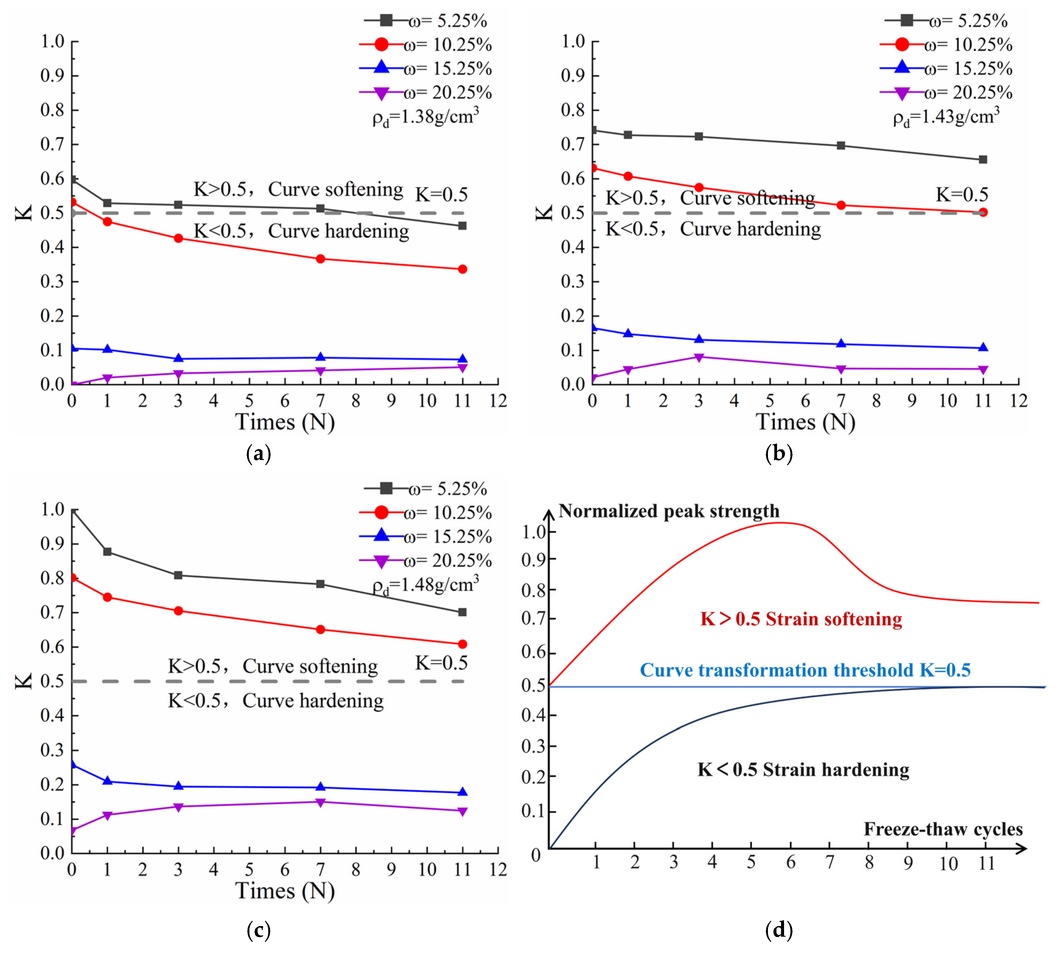
When the soil’s water content is high and its dry density is low, the strength curve is of the hardening type. The soil cannot reach its peak strength at this point, so the stress corresponding to an axial strain of 15% is taken as the peak strength instead. The residual stress cannot be obtained directly at this point. Based on the above test results, the ratio of residual strength to peak strength is used as an empirical value, $\phi$, for the residual strength of the hardening curve.

$${\left({\sigma }_1-{\sigma }_3\right)}_{\mathrm{r}}=\phi ({\sigma }_1-{\sigma }_3{)}_{\mathrm{C}}$$

(30)

Based on the experimental results, the average of $\phi$ was determined to be 0.8.

4.2. Model Validation

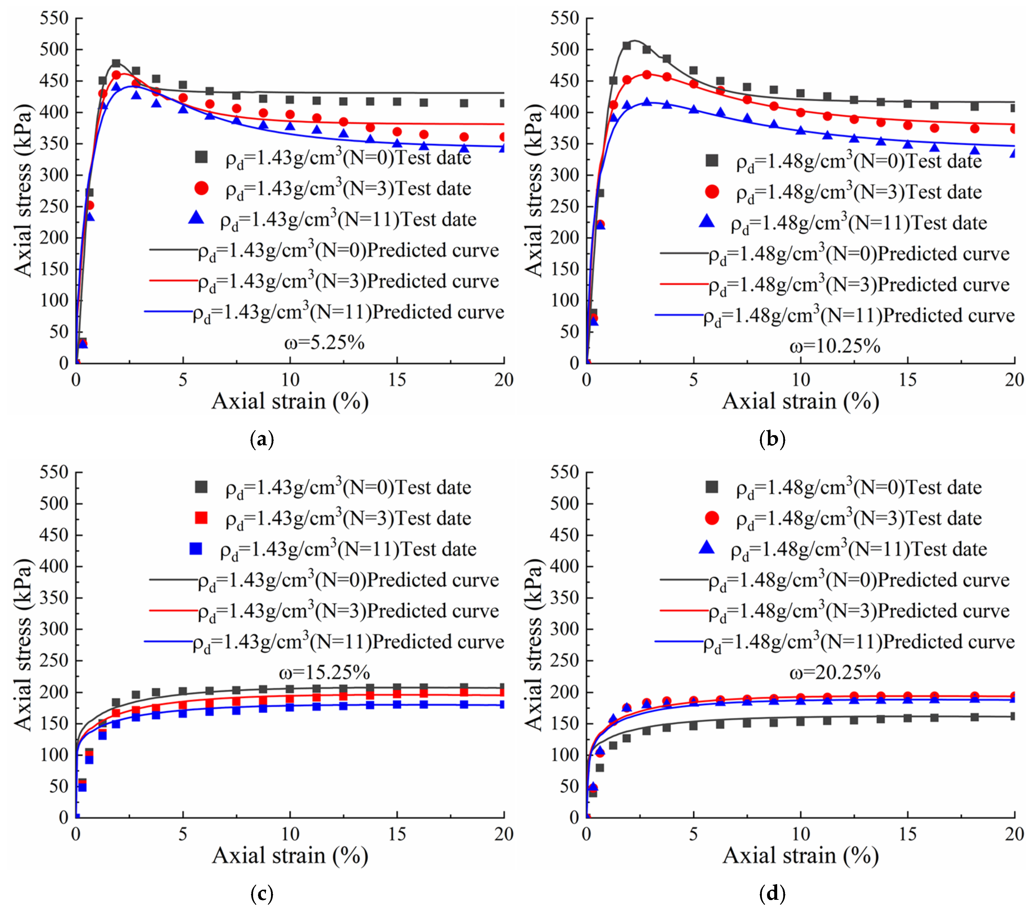
The statistical constitutive model of loess damage established in this paper was verified using unconsolidated undrained triaxial test data. Examples with water contents of 5.25% and 15.25% and dry densities of 1.43 g/cm³, as well as examples with water contents of 10.25% and 20.25% and dry densities of 1.48 g/cm³ were used for this verification. When K > 0.5, the residual strength can be obtained directly from the stress–strain diagram. When K < 0.5, the residual strength is estimated using the empirical value of $\phi$. The parameters required for the model can be obtained from

Table 4. Parameter values for $\omega = 5.25\%$, ${\rho }_{\mathrm{d}}= 1.43{ \mathrm{g}/\mathrm{cm}}^3$ (K > 0.5).

$\mathbf{N}$/Times	${\mathbf{E}}_{\mathbf{n}}/\mathbf{kPa}$	${\left({\mathbf{\sigma }}_1-{\mathbf{\sigma }}_3\right)}_{\mathbf{r}}/\mathbf{kPa}$	$\mathbf{\alpha }$	$\mathbf{\beta }$	$\mathbf{\gamma }$	$\mathbf{m}$	${\mathbf{\epsilon }}_0$
0	456.28	381.28	1.00	1.00	0.97	1.54	3.59
1	405.03	368.28	0.89	1.00	0.96	1.45	4.11
3	380.26	351.28	0.83	1.00	0.96	1.30	4.80
7	364.4	339.28	0.80	1.00	0.94	1.26	4.86
11	347.28	330.28	0.76	1.00	0.94	1.20	4.89

,

Table 5. Parameter values for $\omega = 10.25\%$, ${\rho }_{\mathrm{d}} = 1.48 {\mathrm{g}/\mathrm{cm}}^3$ (K > 0.5).

$\mathbf{N}$/Times	${\mathbf{E}}_{\mathbf{n}}/\mathbf{kPa}$	${\left({\mathbf{\sigma }}_1-{\mathbf{\sigma }}_3\right)}_{\mathbf{r}}/\mathbf{kPa}$	$\mathbf{\alpha }$	$\mathbf{\beta }$	$\mathbf{\gamma }$	$\mathbf{m}$	${\mathbf{\epsilon }}_0$
0	446.6	406.6	1.00	0.99	1.00	1.32	4.35
1	426.78	388.4	0.96	0.98	1.00	0.95	5.21
3	393.4	373.5	0.88	0.98	1.00	0.87	5.51
7	370.35	361.2	0.83	0.97	1.00	0.82	5.72
11	354.32	333.1	0.79	0.95	1.00	0.77	6.20

,

Table 6. Parameter values for $\omega = 15.25\%$, ${\rho }_{\mathrm{d}} = 1.43 {\mathrm{g}/\mathrm{cm}}^3$ (K < 0.5).

$\mathbf{N}$/Times	${\mathbf{E}}_{\mathbf{n}}/\mathbf{kPa}$	${({\mathbf{\sigma }}_1-{\mathbf{\sigma }}_3)}_{\mathbf{C}}/\mathbf{kPa}$	$\mathbf{\phi }{({\mathbf{\sigma }}_1-{\mathbf{\sigma }}_3)}_{\mathbf{C}}/\mathbf{kPa}$	$\mathbf{\alpha }$	$\mathbf{\beta }$	$\mathbf{\gamma }$	$\mathbf{m}$	${\mathbf{\epsilon }}_0$
0	153.27	207.8	166.24	1.00	0.38	0.88	0.51	28.18
1	147.57	199.3	159.44	0.96	0.38	0.87	0.50	27.46
3	144.08	190.6	152.48	0.94	0.36	0.87	0.49	26.77
7	137.43	185.6	148.48	0.90	0.34	0.84	0.49	26.65
11	131.44	180.3	144.24	0.86	0.30	0.82	0.48	25.40

and

Table 7. Parameter values for $\omega =20.25\%$, ${\rho }_{\mathrm{d}}= 1.43 {\mathrm{g}/\mathrm{cm}}^3$ (K < 0.5).

$\mathbf{N}$/Times	${\mathbf{E}}_{\mathbf{n}}/\mathbf{kPa}$	${({\mathbf{\sigma }}_1-{\mathbf{\sigma }}_3)}_{\mathbf{C}}/\mathbf{kPa}$	$\mathbf{\phi }{({\mathbf{\sigma }}_1-{\mathbf{\sigma }}_3)}_{\mathbf{C}}/\mathbf{kPa}$	$\mathbf{\alpha }$	$\mathbf{\beta }$	$\mathbf{\gamma }$	$\mathbf{m}$	${\mathbf{\epsilon }}_0$
0	121.81	161.9	129.5	1.00	0.26	1.00	0.53	30.61
1	144.70	183.1	146.5	1.19	0.33	1.00	0.49	24.33
3	148.94	194.3	155.4	1.22	0.37	1.00	0.49	23.18
7	152.50	200.8	160.6	1.25	0.40	1.00	0.48	21.67
11	150.53	188.6	150.9	1.24	0.42	1.00	0.48	20.13

, which show the experimental data. The model curve is shown in Figure 15. As Figure 15 shows, under unfrozen–thawed conditions of shallow Ili loess, the theoretical curve of the unconsolidated undrained triaxial test generally agrees well with the experimental values.

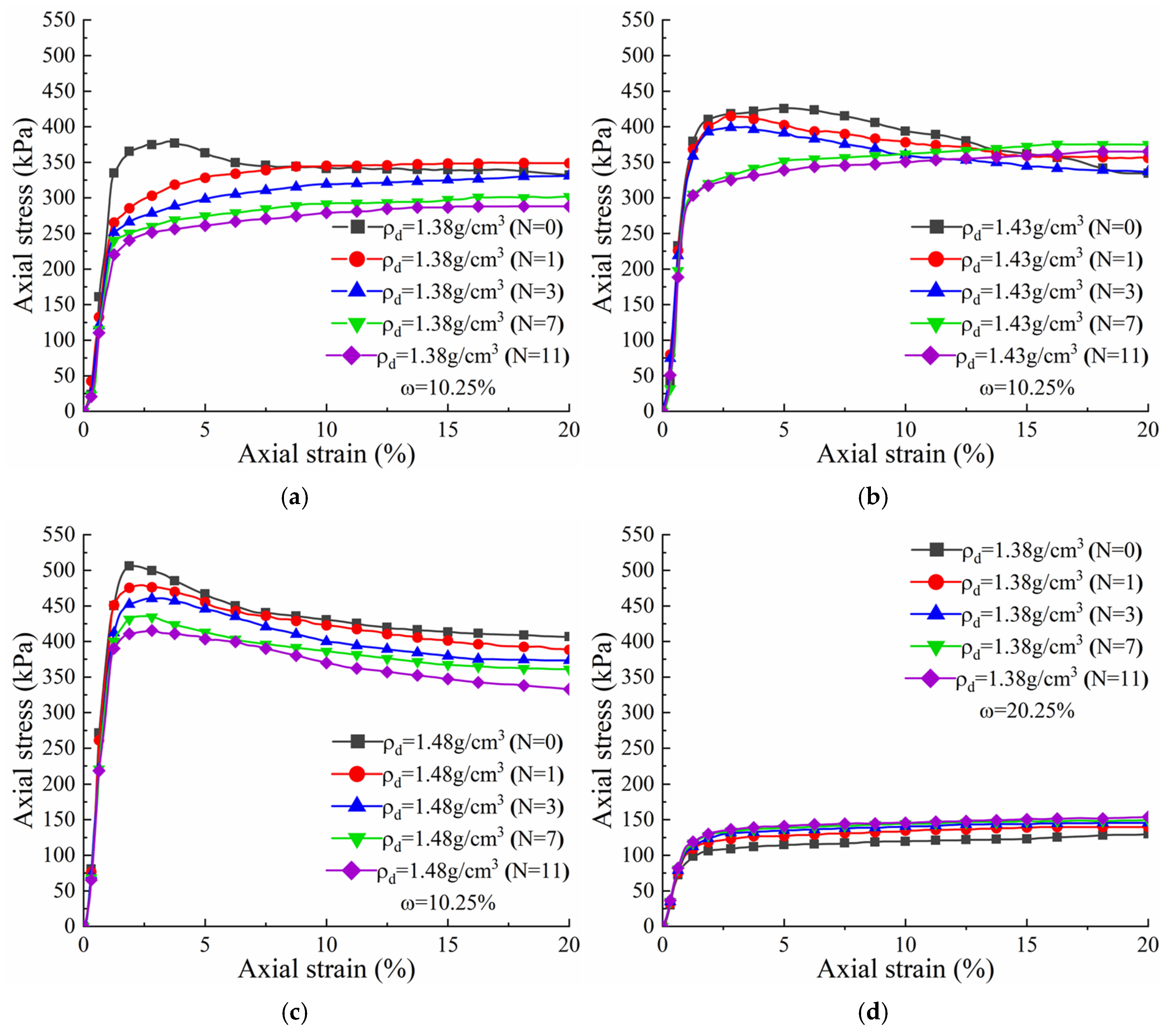
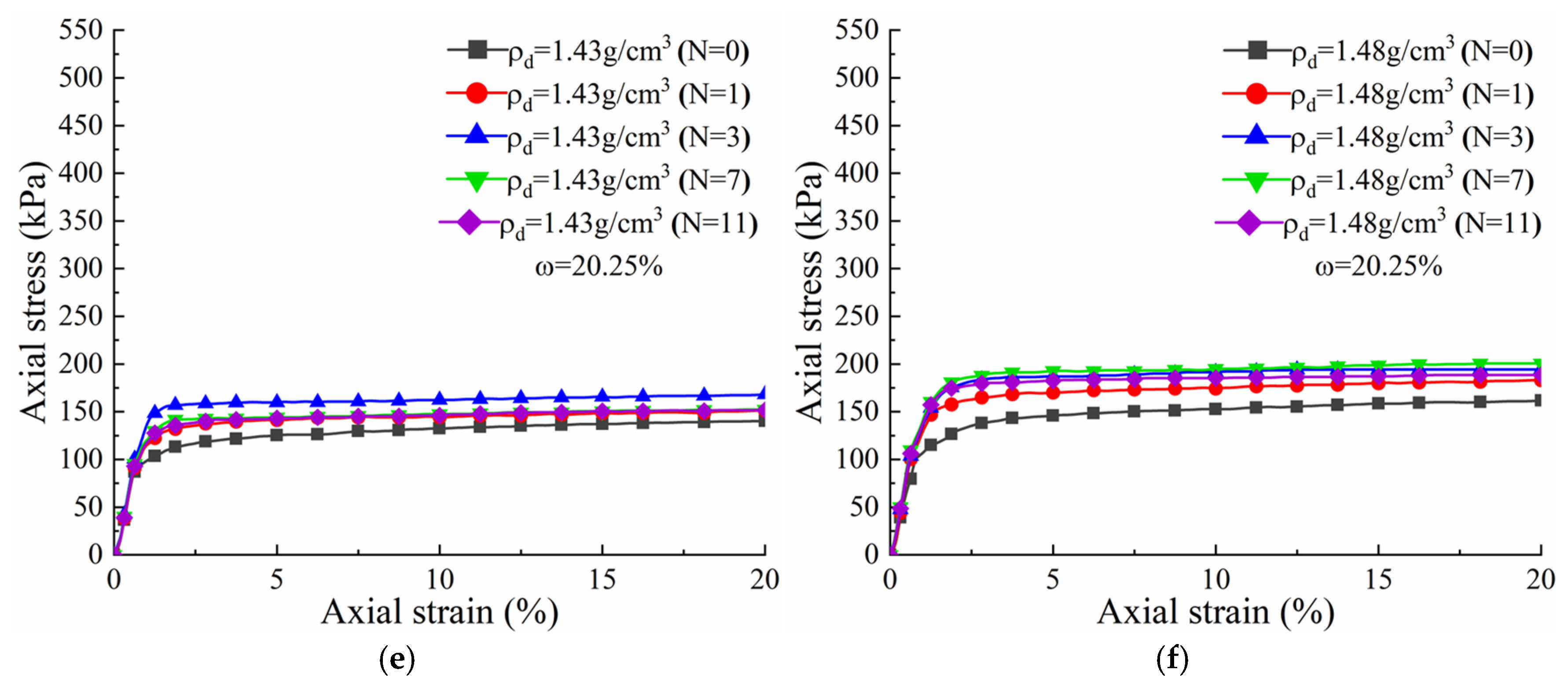
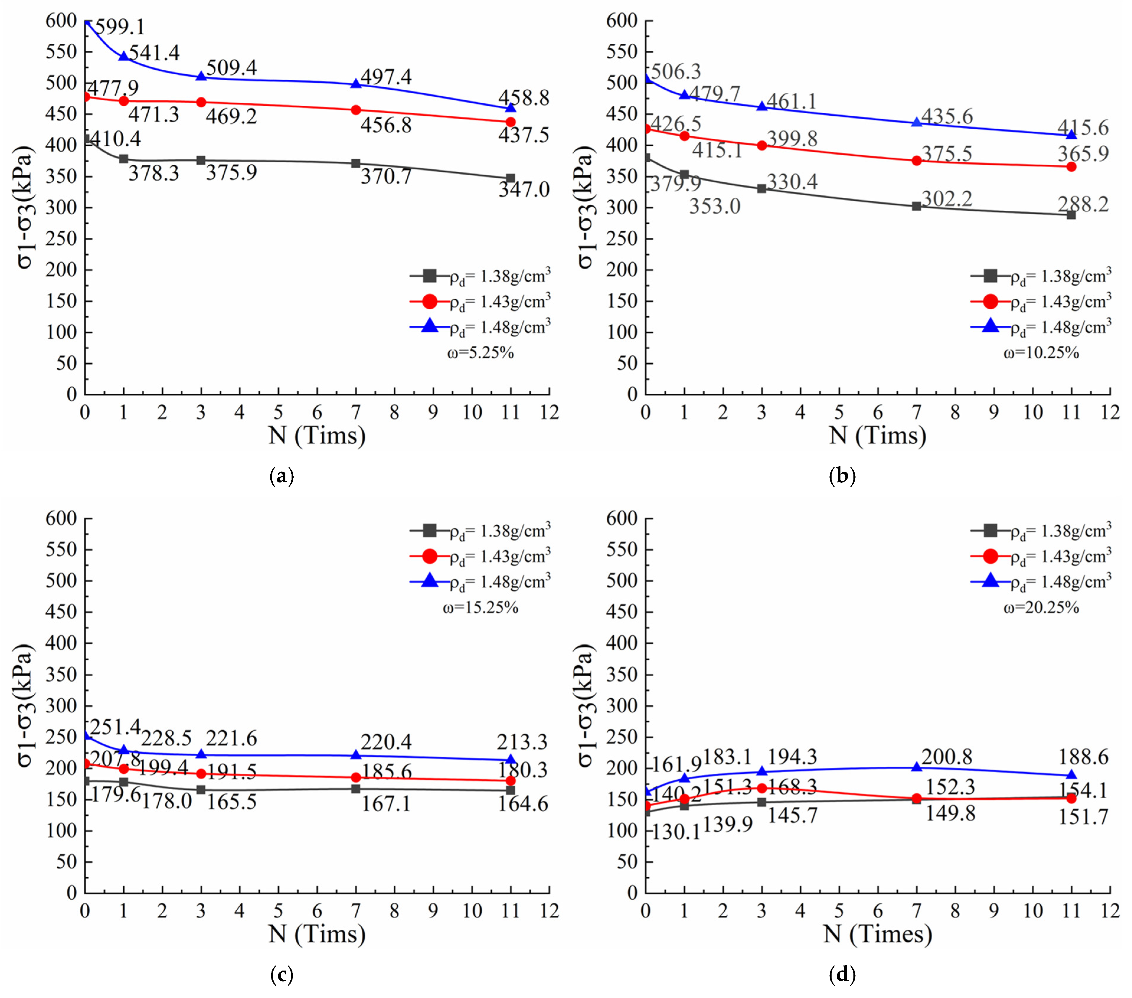
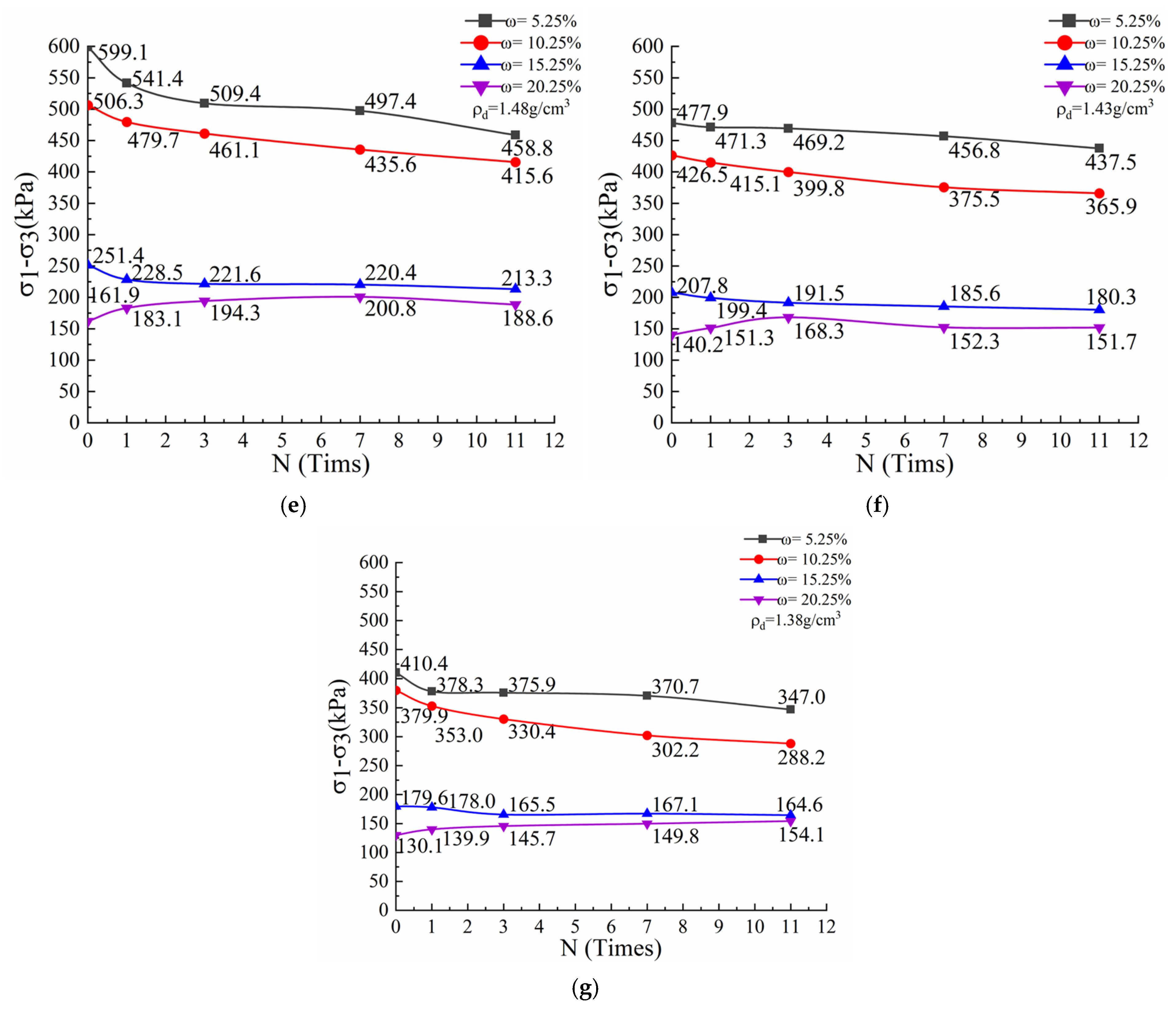
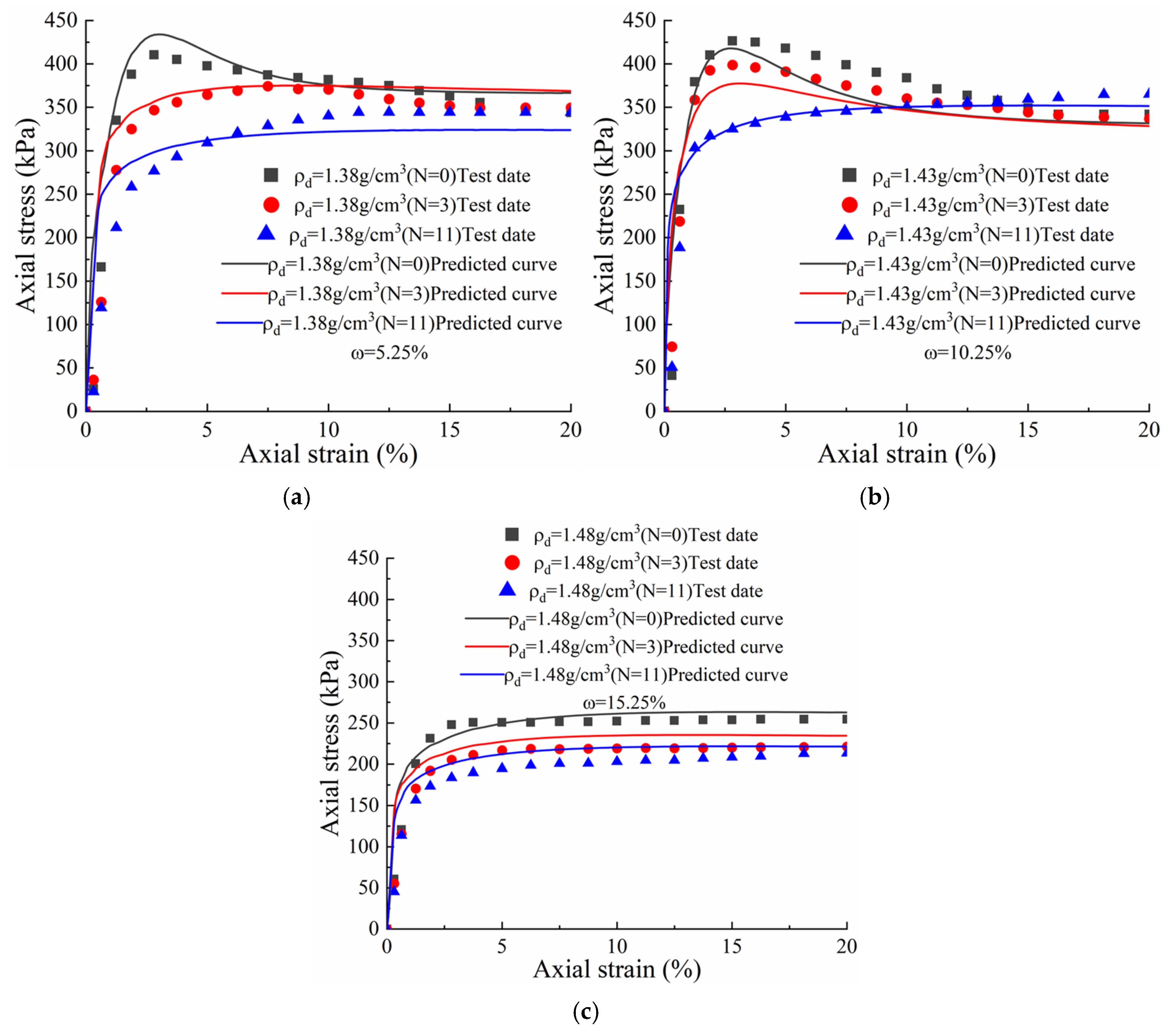
As can be seen in Figure 15, the peak strength of the theoretical curve decreases as the number of freeze–thaw cycles increases. The peak strength also decreases as the water content increases and the curve changes from strain softening to strain hardening. The peak strength of the theoretical curve increases as dry density increases. At a low water content, the curve exhibits strain softening, whereby stress initially increases rapidly before decreasing gradually. Conversely, at a high water content, the curve exhibits strain hardening, whereby the stress initially increases rapidly before slowly rising. The theoretical and test curves exhibit a similar trend. To predict the stress-strain curve under different water contents and freeze–thaw cycles. A relationship be established between the elastic modulus, peak strength and residual strength, corresponding to dry densities of 1.38, 1.43 and 1.48 g/cm³, and freeze–thaw cy-cles and water content. As follows (31):

$$\mathrm{E}={\mathrm{A}}_1-{\mathrm{B}}_1\omega +{\mathrm{C}}_1\mathrm{e}\mathrm{x}\mathrm{p}(-{\displaystyle \frac{\mathrm{N}}{{\mathrm{D}}_1}})-{\mathrm{E}}_1\omega \mathrm{e}\mathrm{x}\mathrm{p}(-{\displaystyle \frac{\mathrm{N}}{{\mathrm{F}}_1}})$$

$${\left({\sigma }_1-{\sigma }_3\right)}_{\mathrm{C}}={\mathrm{A}}_2-{\mathrm{B}}_2\omega +{\mathrm{C}}_2\exp \left(-{\displaystyle \frac{\mathrm{N}}{{\mathrm{D}}_2}}\right)-{\mathrm{E}}_2\omega \mathrm{e}\mathrm{x}\mathrm{p}(-{\displaystyle \frac{\mathrm{N}}{{\mathrm{F}}_2}})$$

$${\left({\sigma }_1-{\sigma }_3\right)}_{\mathrm{r}}={\mathrm{A}}_3-{\mathrm{B}}_3\omega +{\mathrm{C}}_3\exp \left(-{\displaystyle \frac{\mathrm{N}}{{\mathrm{D}}_3}}\right)-{\mathrm{E}}_3\omega \mathrm{e}\mathrm{x}\mathrm{p}\left(-{\displaystyle \frac{\mathrm{N}}{{\mathrm{F}}_3}}\right)$$

(31)

In the formula: $\omega$ is the water content; $\mathrm{N}$ is the number of freeze–thaw cycles; $\mathrm{E}$ is the elastic modulus; ${\left({\sigma }_1-{\sigma }_3\right)}_{\mathrm{C}}$ is the peak strength; ${\left({\sigma }_1-{\sigma }_3\right)}_{\mathrm{r}}$ is the residual strength.${ \mathrm{A}}_1, {\mathrm{B}}_1, {\mathrm{C}}_1, {\mathrm{D}}_1, {\mathrm{E}}_1, {\mathrm{F}}_1, {\mathrm{A}}_2, {\mathrm{B}}_2,{ \mathrm{C}}_2, {\mathrm{D}}_2, {\mathrm{E}}_2, {\mathrm{F}}_2, {\mathrm{A}}_3, {\mathrm{B}}_3, {\mathrm{C}}_3, {\mathrm{D}}_3, {\mathrm{E}}_3,$ and ${\mathrm{F}}_3$ are material parameters related to freeze–thaw testing.

Their calculated values are shown in

Table 8. Parameter values for empirical formulas predicting elastic modulus at different dry densities.

Dry Density (g/cm3)	Predicting Empirical Parameters
	${\mathbf{A}}_{\mathbf{1}}$	${\mathbf{B}}_{\mathbf{1}}$	${\mathbf{C}}_{\mathbf{1}}$	${\mathbf{D}}_{\mathbf{1}}$	${\mathbf{E}}_{\mathbf{1}}$	${\mathbf{F}}_{\mathbf{1}}$
1.38	$249.41$	$6.62$	$134.23$	$2.49$	$7.47$	$2.21$
1.43	$453.99$	$16.71$	$140.03$	$2.22$	$8.09$	$2.10$
1.48	$466.62$	$16.63$	$166.86$	$3.11$	$9.36$	$2.64$

,

Table 9. Parameter values for empirical formulas predicting peak strength at different dry densities.

Dry Density (g/cm3)	Predicting Empirical Parameters
	${\mathbf{A}}_{\mathbf{2}}$	${\mathbf{B}}_{\mathbf{2}}$	${\mathbf{C}}_{\mathbf{2}}$	${\mathbf{D}}_{\mathbf{2}}$	${\mathbf{E}}_{\mathbf{2}}$	${\mathbf{F}}_{\mathbf{2}}$
1.38	$416.73$	$14.43$	$121.50$	$2.49$	$6.49$	$3.41$
1.43	$516.33$	$20.98$	$108.79$	$9.31$	$3.78$	$3.58$
1.48	$583.65$	$20.66$	$187.59$	$2.59$	$10.51$	$2.13$

and

Table 10. Parameter values for empirical formulas predicting residual strength at different dry densities.

Dry Density (g/cm3)	Predicting Empirical Parameters
	${\mathbf{A}}_{\mathbf{3}}$	${\mathbf{B}}_{\mathbf{3}}$	${\mathbf{C}}_{\mathbf{3}}$	${\mathbf{D}}_{\mathbf{3}}$	${\mathbf{E}}_{\mathbf{3}}$	${\mathbf{F}}_{\mathbf{3}}$
1.38	$337.81$	$11.01$	$128.56$	$5.99$	$7.54$	$7.41$
1.43	$405.97$	$16.06$	$95.37$	$7.65$	$3.74$	$3.57$
1.48	$438.05$	$16.40$	$124.55$	$7.91$	$5.37$	$3.97$

. The strength parameters are calculated using the above equation and then substituted into the constitutive model to obtain the predicted curve. This curve is then plotted and compared with the experimental data, as shown in Figure 16.

The inaccuracies between the experimental values and theoretical values of the elastic modulus, peak deviation stress, and residual deviation stress is obtained by comparing the predicted curve with the experimental curve. The inaccuracies between the experimental values and the predicted theoretical values is calculated using the following Equation (32):

$$\mathrm{R}\mathrm{e}\mathrm{l}\mathrm{a}\mathrm{t}\mathrm{i}\mathrm{v}\mathrm{e} \mathrm{e}\mathrm{r}\mathrm{r}\mathrm{o}\mathrm{r}={\displaystyle \frac{\left|{\mathrm{T}}_{\mathrm{i}}-{\mathrm{P}}_{\mathrm{i}}\right|}{{\mathrm{T}}_{\mathrm{i}}}}\times 100\%$$

(32)

In the equation: ${\mathrm{T}}_{\mathrm{i}}$ is the experimental test value, ${\mathrm{P}}_{\mathrm{i}}$ is the empirical predicted value, and $\mathrm{i}$ represents the elastic modulus, peak strength, or residual strength. It can accurately predict within 20%, referencing Figure 17. It is evident that Equation (31) provides relatively accurate predictions for soil strength, elastic modulus, and residual strength, thereby offering theoretical support for engineering projects in the Ili region.

In summary, the constitutive model established in this paper effectively predicts the mechanical characteristics of Ili loess under wet–dense-freeze–thaw cycles. The overall trend is consistent with the experimental results and reflects the changes in damage to the stress–strain relationship of Ili loess under cyclic conditions. Consequently, the proposed damage statistical constitutive equation can relatively accurately describe the strength and damage characteristics of Ili loess in the Xinjiang region.

5. Discussion

This study experimentally investigates the degradation of mechanical properties, volume changes, and surface deterioration in soils subjected to varying water contents, dry densities, and freeze–thaw cycles. Parametric analysis was conducted on water content, dry density, and damage induced by freeze–thaw cycles during the damage process, though numerical simulations and microscopic experiments were not performed. Internationally, microscopic experiments primarily focus on soil internal pores, particle size, particle shape, and inter-particle contact mechanisms [57,58,59]. This study demonstrates significant alterations in soil volume and surface degradation due to changes in constraint conditions. Subsequent SEM experiments [60,61] will be conducted and compared with prior studies to elucidate, from a microscopic perspective, the effects of confinement conditions on soil strength and internal structure. The following outcomes may be observed: Firstly, particle size degradation is reduced, with particles exhibiting larger diameters relative to those in top-constrained soils. This indicates that without top confinement during freeze–thaw cycles, frost heave forces induce substantial volume changes while minimising damage to larger particles. Secondly, the upper and middle sections of the soil (where according to experimental research, the upper 10 mm exhibits significant volume change and is comparatively looser than the lower sections) show larger pores than the top-constrained soil. Thirdly, the particle shapes feature fewer rounded grains and more point contacts between particles. Beyond microscopic explanations, subsequent research will also involve numerical simulation studies. Reviewing the prior literature reveals that optimising boundary conditions can yield numerical simulation results closer to real-world conditions [31,32,33]. Subsequent studies will employ finite element software [62,63,64] and discrete element software [65] to further analyse the micro- and meso-scale failure mechanisms of without top constraint Ili shallow loess under freeze–thaw cycling conditions.

6. Conclusions

This paper presents a method of artificially preparing samples shallow Ili loess in order to simulate the effects of freeze–thaw cycles on soils under natural conditions. This enables the damage process to be observed. Freeze–thaw cycle tests and triaxial tests were conducted to study the strength and height changes as well as the surface degradation of shallow Ili loess under freeze–thaw cycles. Threshold conditions for the transition from softening to hardening in the stress–strain curve were identified, and a three-factor damage constitutive model was established under wet–dense-freeze–thaw conditions. The following conclusions were drawn:

• Shallow Ili loess strength decreases with an increasing number of freeze–thaw cycles but slightly increases at a water content of 20.25%. Soil strength is most affected by water content, followed by dry density. When the water content and dry density are low, fewer freeze–thaw cycles are needed for the stress–strain curve to change from softening to hardening; at a high water content, the curve is entirely hardening. When the normalised strength K is less than 0.5, the soil strain curve hardens; when K is greater than 0.5, the soil strain curve softens.
• When subjected to freeze–thaw action, the height of unsaturated shallow Ili loess changes little at low and near-optimal water content; however, significant changes in height occur when the water content increases, especially above the plastic limit, and under saturated conditions. The degradation of saturated soil surfaces worsens with the number of freeze–thaw cycles. At a specific dry density, the height change exhibits a dynamic phenomenon of first increasing, then decreasing, and then increasing again.
• The proposed damage coefficient that considers the initial water content, dry density, and number of freeze–thaw cycles. A coupled damage constitutive model that considers the three aforementioned factors and satisfies the shallow Ili loess is established. This model can relatively accurately predict changes to the stress–strain curve of shallow Ili loess under wet–dense-freeze–thaw conditions.

Following the aforementioned experimental investigations, several shortcomings are apparent. Firstly, the confining pressure and stress path configurations were inadequate, with no comparative analysis of strength parameters (such as internal friction angle and cohesion). Secondly, experiments were conducted solely on remoulded soil, lacking comparison with undisturbed soil and without SEM analysis to contrast the internal structures under the two confinement states. Thirdly, experimental findings were not cross validated through numerical modelling. Subsequent research will address these gaps through further investigation and refinement.

7. Patents

Shihezi University. A sampling mould, freeze–thaw box, and method considering changes in soil volume:CN202410813399.9[P]. 27 September 2024.