Application of Innovative Artificial Intelligence Methods to Detect Flat Feet in Children

Abstract

This study examined the potential of artificial intelligence tools for detecting pediatric flatfoot pathology. We would like to emphasize that there is very little research in this area and we would like to point out that this is a relevant and very important topic in medicine. First, the base flow was used: a pre-trained “backbone” on the ImageNet platform. In this study, this term is used to describe the feature extraction part of a convolutional network. A standardized pre-processing with pruning and augmentation was performed, and a three-stage training schedule (stages 1, 2 and 3), average and maximum aggregation at the subject level and the addition of light test time were proposed. Eight different model architectures were used. From stage 2 onwards, all models were trained on feet. Three-dimensional photographs with real flatfoot shapes, from flatfoot stages I to III, were used. The most validated model was displayed in accurate AUROC plots with estimated average and maximum aggregation values with standard deviation. The research and calculations conducted demonstrate the possibility of applying artificial intelligence in the field of orthopedics.

1. Introduction

Flat feet are a common problem for patients visiting any musculoskeletal clinic. This condition, often called pes planus, planovalgus foot, or simply fallen arches, can be congenital or acquired. All people are born with flat feet and this lasts until about 3 years of age, because children have a fatty layer on their feet and are not yet walking steadily. After they start walking normally, when the feet are loaded, the ligaments and muscles strengthen and the arches of the feet begin to form. As many as 95% of people acquire flat feet and only 5% have it congenitally [1,2,3,4,5,6]. Flat feet deformities in children usually correct spontaneously during the first decade of life and usually do not require special treatment [7]. Flat feet are normal in young children and sometimes persist into adulthood without any symptoms. Although flat feet in childhood are usually associated with immaturity, they can be associated with neuromuscular diseases, laxity syndromes, and many other causes. If left untreated, flatfoot can gradually become symptomatic, causing pain and disability [8,9]. There are many causes of acquired flatfoot, including posterior tibial tendon degeneration, trauma, neuroarthropathy, neuromuscular disease and inflammatory arthritis. Of these, tibial tendon degeneration is probably the most common. The foot is distinguished from other parts of the body by its contact with the ground during movement, which is why its structure and function are so important. Each bone connects to another, forming a closed movement system, through which each movement disorder reaches other parts of the system: the knee, hip joints, back and neck [10,11,12]. The foot is unique in that it is in contact with the ground during movement, which is why its structure and function are so important. Each bone connects to the other, forming a closed movement system, through which any movement disorder reaches other parts of the system: the knees, hips, back and neck [11,12,13].

Anatomically, it is accepted that the foot consists of three parts—the ankle, which allows the shin bones to connect to the foot, the midfoot, and the toes. The main function of the ankle and foot is to absorb shock and generate force when walking. The sole absorbs (absorbs) most of the load on the body, but if the foot does not perform its function properly, other parts of the body (knees, hips, spine, etc.) receive increased load, which can eventually lead to damage to the musculoskeletal system [14,15,16]. At first glance, the foot may seem like a simple part of the body that does not require much attention, but when we look at it anatomically, we can see that the foot is a complex assembly of bones, muscles, ligaments, and joints. In flatfoot, the arches of the feet descend downward, and the foot itself turns inward. Flatfoot is influenced by weakness of the ligaments and muscles, so the correct shape of the arches is not maintained. If the arches do not form, the entire posture of a person is disrupted [15,16,17,18].

The aim of this work was to apply artificial intelligence methods and to detect flat feet in children.

Recently, various artificial intelligence tools have been widely used in almost all fields. The field we are considering is no exception. There is a publication that attempts to determine whether a pathology is present or absent from a camera image [19]. The article examines lateral images of the foot, such images are not widely used in the field of orthopedics. In our publication, we present a scan of the foot from below. By applying various artificial intelligence tools, we will determine the presence/absence of flatfoot.

2. Foot Function, Biomechanics and Pathology

In order to apply AI tools correctly, it is first necessary to understand and know the function and anatomy of the foot. Therefore, this chapter introduces the anatomy, biomechanics and pathology of the foot.

2.1. Foot Function

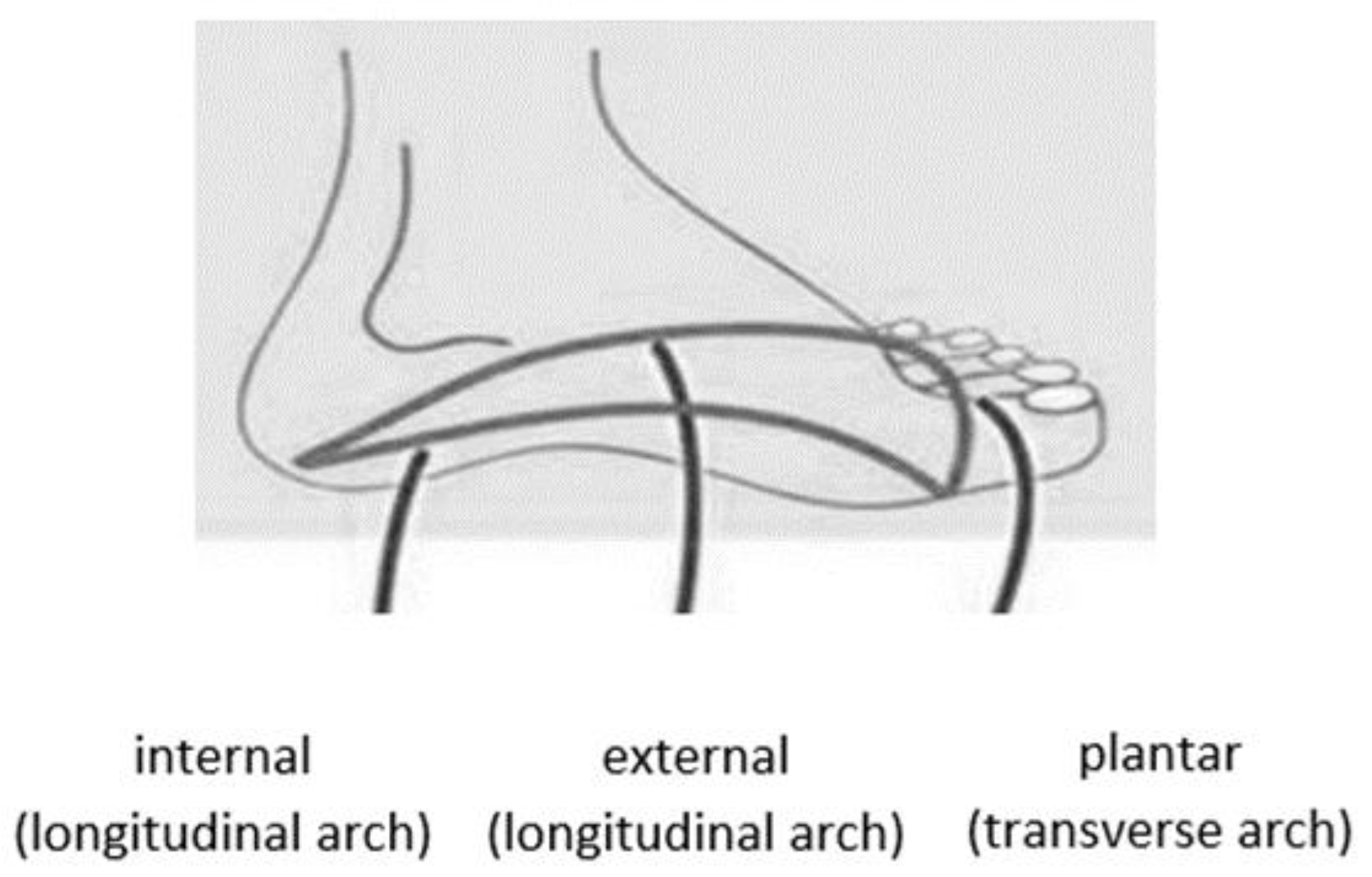
The foot has a double arch: longitudinal and transverse. The foot has three arches and presented in Figure 1 [11,20,21]:

• The lateral longitudinal arch, which is the arch on the outer side of the foot. This arch is responsible for supporting the foot, and the force of the body’s weight is transmitted through it from the lower leg.
• The medial longitudinal arch, which is the arch found along the inner part of the foot, is characterized by soft tissues and interarticular cartilage. The purpose of the medial longitudinal arch is to cushion contact with the ground.
• The transverse arch of the foot is located across the foot, connecting the first and fifth metatarsals.

Figure 1. The foot arches.

Figure 1. The foot arches.

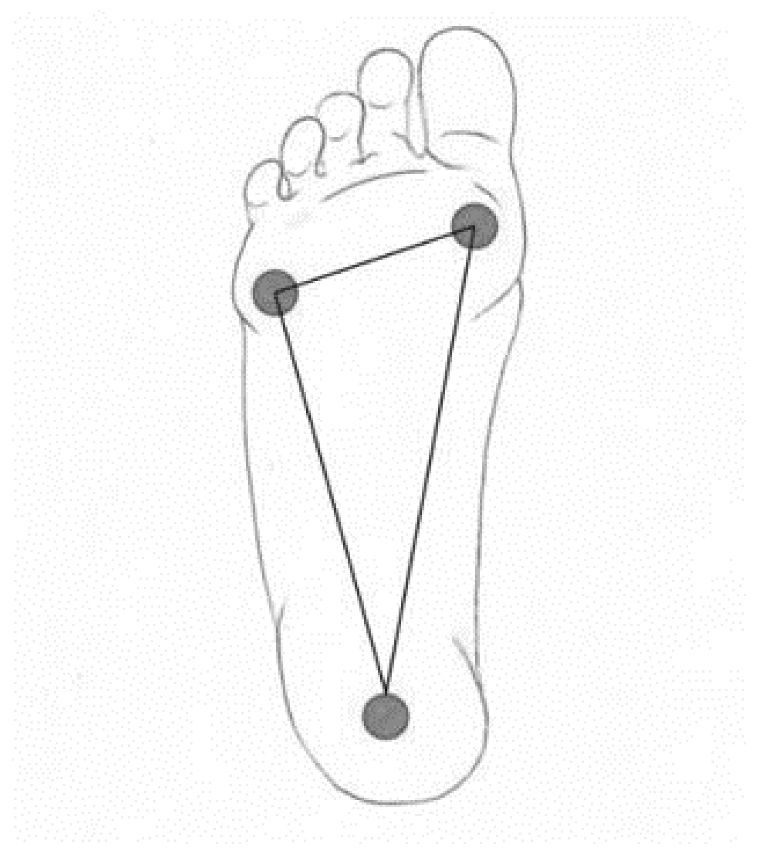
The calcaneus is a common bone of both the outer and inner arches. The inner arch consists of the calcaneus, the talus (through which the foot connects to the arch), the navicular bone, three arches and the I–III metatarsals. The outer arch consists of the calcaneus, cuboid bone, the IV and V metatarsals. Ligaments and muscles influence the shape of the arches. The arches of the feet fluctuate depending on the load. On the inner side, 5–7 cm, and on the outer side, about 2 cm. The most significant part in maintaining the shape of the arches is the lintel stone, it is located at the top of the arch and connects the arcuate bridge or arcuate gate structure. The foot has one scutellum in each arch. These scutella are the scutellum, the talus and the inner scutellum. The base of the foot consists of three main support points—the base of the calcaneus, the head of the I metatarsal with two sesamoid bones, and the head of the V metatarsal. In a healthy foot, all three points distribute the load and connect into a triangle with the help of arches (Figure 2) [8,22,23].

The base of the foot (3 support points) is extremely important for the body’s balance and posture. If the work of the muscles is disturbed, this changes the biomechanics of walking and the support points can change, causing irregular posture, coordination problems, and joint and bone deformities.

2.2. Foot Biomechanics

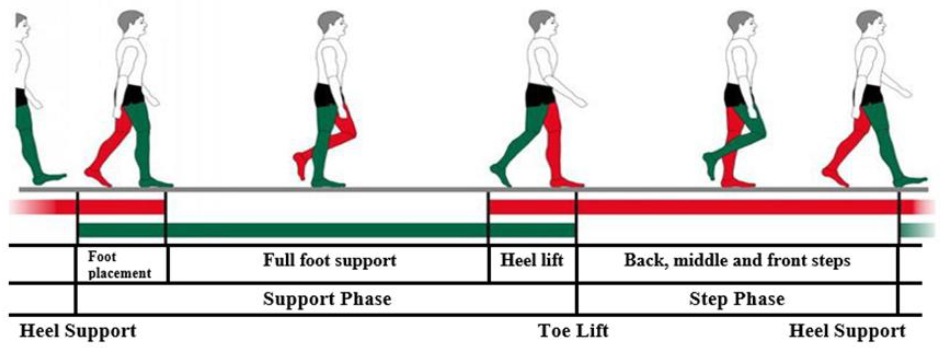
Figure 3 shows the biomechanics of the human foot. The body load is transmitted from the lower legs to the feet through the talus. In the standing position, the talus transfers the load to the calcaneus and the heads of the I and V metatarsals. When taking a step with the heel on the ground, the force of the body weight on the foot is transmitted to the calcaneus, and when the angle of the lower leg reaches 90 °C with respect to the ground, the load is distributed to the heads of the I–V metatarsals and the big toe. Passive and active forces help maintain the anatomically accepted average height of the arches. Passive force is influenced by the work performed by the ligaments and joints to maintain the bones of the foot in a single common structure. Muscles influence the active force, since the muscles and ligaments create the necessary flexibility for the arches of the foot, which ensures the rise and fall of the arches during movement [15,23,24,25].

The strongest ligaments are found in the ankle. They connect in different directions. On the inside of the ankle joint is the triangular-shaped deltoid ligament. The beginning of this ligament is considered to be the medial malleolus of the tibia, and the deltoid ligament expands to four fibers, with which it is attached to the navicular bone, talus and coccyx. It strengthens the ankle joint on the inside, holding the calcaneus and navicular bone in place in front of the talus. On the side of the ankle joint is the external ligament, which consists of three parts extending from the external malleolus of the fibula to the talus and calcaneus, these three parts strengthen the structure of the external longitudinal arch of the foot. The foot is strong due to the connections of the bones and ligaments in it, but physical activity is also extremely important for maintaining strength. The muscles in the feet are found on the inside and outside, but the strongest are on the sole. These muscles are divided into the intrinsic and the foot-lowering muscles. The lower limbs are also divided into the muscles of the sole and the top of the foot.

Muscles perform extremely important functions in the feet, because thanks to them, actions are performed in the joints after receiving nerve signals, the work of the muscles helps to adjust the body’s balance and its correct alignment. The arches are supported by the plantar muscles, which connect the heel with the front of the foot, and the calf muscles, which raise the edges of the arches. When a healthy foot is exposed to load, the arches rise and maintain their shape, due to the work of the muscles and ligaments. Two important tendons operate in the foot—the broad one, which is found almost throughout the entire foot from the heel bone to the metatarsals, and the Achilles tendon, which connects the heel bone and reaches the middle of the calf.

A healthy foot rotates slightly inward and touches the ground with the outer side. This provides cushioning and eases the impact of the ground during walking, thus accumulating force that carries the body forward. The biomechanics of the foot are complicated because movements are performed in different planes at the same time. Inversion is when the foot is turned inward, and eversion is when the foot is turned outward. When the foot is turned inward at the ankle, it can flex and extend, but the foot still performs the functions of abduction and adduction.

The biomechanics of the foot consist of active supporting and passive unsupported movements. During passive unsupported movements, the heel performs inversion and eversion of the hindfoot about the metatarsal joint. By limiting heel movement, it is possible to passively abduct the forefoot, elevate, rotate, flex, and extend the metatarsal joints of the toes and ankle. For active supporting movements, it is common for weight forces and muscle work to stabilize the joints. When moving at an average pace, about sixty steps are taken per minute, and as many as 62% of all steps are made up of support. The support period consists of a double support, during which both feet, which are not in the same phase, are supported on the ground. The bridge phase is longer if the movement is faster.

In standard movement, about 15% of the support time, the foot rotates to the inner side. In the action of placing the foot and lifting the heel, the foot turns to the outer side and weighs down. When the foot rotates, the talus contributes, so when the toes rise up, the foot is rotated to the outer side the most. During rotation, the foot is strengthened by ligaments and muscles.

2.3. Flatfoot Pathology

In flat feet, the arches of the feet descend downwards, and the foot itself turns inwards. Flat feet are influenced by the weakness of the ligaments and muscles, so the correct shape of the arches is not maintained. If the arches are not formed, the entire posture of the person is disturbed. The most common reasons for acquiring flat feet at a young age are overweight and low physical activity, so it is extremely important for children to be active.

According to the World Health Organization, one fourth of the younger population of Lithuania is overweight. A study conducted in 2015–2017 showed that 12% of boys and 8% of girls are obese, and as many as 28% of boys and 23% of girls have overweight disorders. Poor nutrition and very little physical activity increase the risk of flat feet. This study also found that 2 out of 5 children come to school by car and 1 out of 5 children come by bus [26]. 39% of students participate in extracurricular sports activities and at least 50% of children spend at least 2 h a day in front of smart device screens. Over time, children’s physical activity is decreasing and the problem of flat feet is becoming more common. Due to low activity, the foot muscles are extremely sluggish, so all the load is transferred to the ligaments, which become very tense and the foot becomes stiff, and the ligaments are no longer able to support the arches of the foot and they sag. Finally, the bones of the foot are also damaged, so the foot is no longer able to cushion the shocks received from the ground during walking. Another very common cause of flat feet is footwear that injures the feet. It is highly recommended to walk barefoot and be able to choose the right footwear [7].

Walking barefoot activates the muscles and ligaments of the legs. During walking barefoot, the whole organism is activated, because the corresponding points are pressed, which are transmitted further by nerve impulses. Walking on different natural surfaces has a significant impact on preventing flat feet. Walking barefoot has a significant impact not only on the structure of the foot, but also on the psycho-emotional state of a person. Orthopedist Dr. Hoffman notes at the end of the study that, after reviewing 186 primate feet, no signs of muscle weakness were observed, which is common when wearing footwear, since it limits the function of the feet. Babies should not be taught to walk very early, because their feet are not used to such loads and this overexerts the muscles of the feet. It is healthiest to teach babies to walk only when they are about seven months old and to hold them by the shoulders, armpits and hips.

Acquired flat feet are classified according to the Johnson and Strom classification system, which has classification degrees from I to III. In 1997. Merson added a fourth grade. The grading system helps clinicians determine the severity of AAFD and can be used to guide treatment plans. Stage I is characterized by tenosynovitis of the posterior tibial tendon without collapse of the arch. Patients with stage II adult-acquired flatfoot have collapsed feet and are unable to perform a single-leg heel raise. This stage is further divided into stages IIa and IIb. Stage IIa has a foot drop with a valgus deformity of the hindfoot but no midfoot abduction, while stage IIb has midfoot abduction. Patients with stage III adult-acquired flatfoot have a fixed deformity with valgus deformity of the hindfoot and abduction of the forefoot. Patients with stage IV deformity have ankle valgus due to weakening of the deltoid ligament [2,3,4,5,6]:

• Stage I. Stage I is the mildest form of PTT dysfunction. Patients may have a history of tenosynovitis or tendinosis with mild to moderate pain along the tendon course. The hindfoot is mobile and normally flexed. The PTT can still invert and lock the hindfoot during heel-lift, allowing the patient to stand on the toes. Radiographs may be normal, although MRI may show PTT inflammation or early signs of degeneration.
• Stage II. In stage II, deformity and impaired function develop. However, the deformity is still flexible and passive correction can be achieved by adducting and inverting the metatarsal joint. As the PTT degenerates and lengthens, the foot inverts less actively, and the transverse metatarsal joints can no longer be locked and the toes can no longer be supported. Later, the bones distal to the talus rotate laterally, and the talocrural joint subluxes, resulting in hindfoot valgus and forefoot abduction. The unsupported talus is now plantarflexed. At some point, the spring ligament may weaken, which may contribute to the increase in deformity. A stage IIA deformity is characterized by minimal abduction at the midfoot and less than 30% tarsal coverage on a standing AP radiograph. A stage IIB deformity is still flexible, but there is greater forefoot abduction (>30% tarsal coverage). The distinction between stages IIA and IIB may help determine the treatment approach.
• Stage III. Stage III represents a more fixed deformity, where correction by passive inversion to neutral is no longer possible. The hindfoot is in a fixed valgus position, while the forefoot is abducted.
• Stage IV. A stage IV deformity differs from the other stages in that the ankle joint is involved. In stage IV, the deltoid ligament is insufficient, resulting in lateral talar tilt and valgus deformity of the tibia. Although some patients have tibial deformity and flexible flatfoot (called stage IVa), most patients have rigid foot deformities due to damage to the ankle joint (called stage IVb). In addition to tibial deformity, arthritis of the ankle joint may also be present. Uncorrectable flatfoot is characterized by impaired foot support, gait changes, discomfort when standing or walking, rapid fatigue in the foot area, and coordination changes.

However, we do not adhere to this scale, since it is recommended for adults, as mentioned above, to assess the form of acquired flatfoot, which most often occurs due to degenerative changes in the tendons, injuries or overloads. This pathology is almost not characteristic of children, so it is more appropriate to apply and discuss the FPI scale (Foot Posture Index):

• Stage I. Stage I is the easiest/mildest degree. Foot fatigue is felt when walking or running. It is uncomfortable to wear shoes, pressure is often felt. Edema appears. The shape of the foot remains physiological. The arch height is 25–35 mm. The arch angle is 131–140 degrees.
• Stage II. Stage II is an average/intermittent degree. Pain can be felt not only in the feet, but also in the calves, after short walks or standing. Gait and posture disorders appear. A distinctive feature of the second degree of flatfoot is that the longitudinal arch of the foot flattens out during the day, and in the morning, it returns to its previous state. The height of the arch reaches 24–17 mm. The angle of the arch is 141–155 degrees.
• Stage III. Stage III is the most severe degree of flatfoot. The pain felt covers the feet, calves to the kneecap. The pain makes it difficult to walk or engage in any physical activity. Due to the severely deformed foot, its biomechanics are disrupted, which provokes other serious pathologies such as scoliosis, arthritis and arthrosis. The height of the arch reaches 17 mm and below. The angle exceeds 155 degrees.

This assessment scale is also suitable for determining the posture of the foot in adults. The assessment scale is used to assess the position of the foot (pronation-supination) and determine whether the foot is: supinated, neutral, pronated/flatter. This is not a direct diagnosis of “flatfoot”, but a very good tool for assessing foot posture and monitoring changes. Other methods:

• Clinical examination (assessment of arch height, heel axis, gait);
• Standing on tiptoes (if the flexible arch is restored—this is physiological flatfoot);
• Photopodometry or plantography;
• Jack test (restoration of the arch of the foot by lifting the toe);
• X-ray—only if additional diagnostics are needed.

Orthopedic care is the selection of orthopedic devices. Their range is extremely wide, including half- and full-foot inserts, footwear and insoles, but they are not effective if the stage of flatfoot is determined incorrectly. Therefore, after reviewing all the main features of the anatomy, biomechanics and pathology of the foot, we can use artificial intelligence tools and determine the presence/absence of pathology.

3. Application of Artificial Intelligence Tools for Pathology Detection

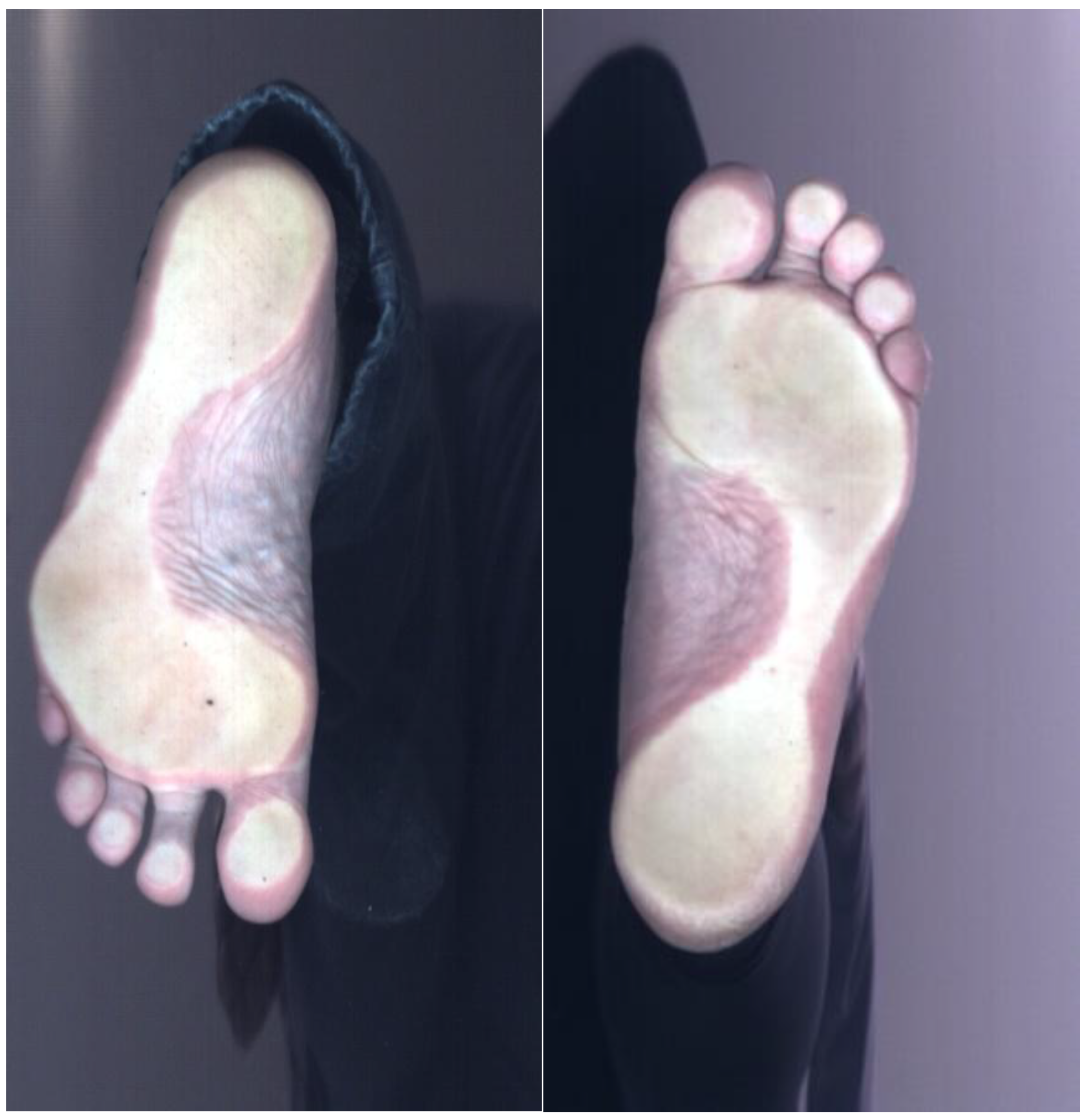
This investigation presents a methodology based on the application of artificial intelligence tools to identify flatfoot pathology in children. Using the Elinvision iQube scanner, 2D images were measured, reflecting the structure of the patient’s foot. The scanner accuracy 0.5 mm, scanning area (L × W × H) 40 × 180 × 150 mm ± 5 mm; scan time is 5–9 s; file format—png; heel positioning laser Integrated heel positioning laser allows to align patient’s foot/ankle for the better scan result; 3D texture in color allows to view and evaluate the condition of the sole and markings made by physicians; calibrated 2D texture in color provides more accurate data in images. The dataset comprised 42 pediatric subjects, each contributing two plantar images (left and right foot), for a total of 84 images. The age of the patients was from 3 to 14 years. Clinical labels were provided at the subject level and mapped to both feet: 33 subjects were classified as healthy and 9 subjects as flatfoot (see

Table 1. Dataset summary.

	Number of Subjects	Number of Images
Controls (no flatfoot)	33	66
Flatfoot	9	18
Total	42	84

). Only binary labels (healthy vs. flatfoot) were available; no gradation of flatfoot severity (e.g., stages I–III) was provided. Labels were assigned as healthy vs. flatfoot by a pediatric orthopedist. Children classified as having flexible flatfoot according to routine clinical assessment were labeled as ‘flatfoot’. Asymptomatic children with a normal medial longitudinal arch and neutral hindfoot alignment were labeled as ‘non-flatfoot’. All “flatfoot” cases (regardless of suspected stage) were merged into one positive class. For this study, a binary label (flatfoot vs. non-flatfoot) was used. Stages were not modeled separately due to the small sample size. Signed written consent to participate in the study was obtained from all subjects. The study was conducted in accordance with the ethical principles of the Declaration of Helsinki (64th WMA General Assembly, Fortaleza, Brazil, October 2013). Identifiable information was removed from the collected data to ensure subject anonymity. An example of the images used is shown in Figure 4. Standardization and sorting of scanned data (e.g., consistent foot positioning, illumination) were performed to ensure data uniformity and reliability. Analysis of existing databases and diagnostic tools applied to 3D image processing and classification, e.g., specialized 3D CNN architectures or hybrid models that combine 3D geometric analysis with 2D feature extraction.

3.1. Study Workflow and Backbone Methods

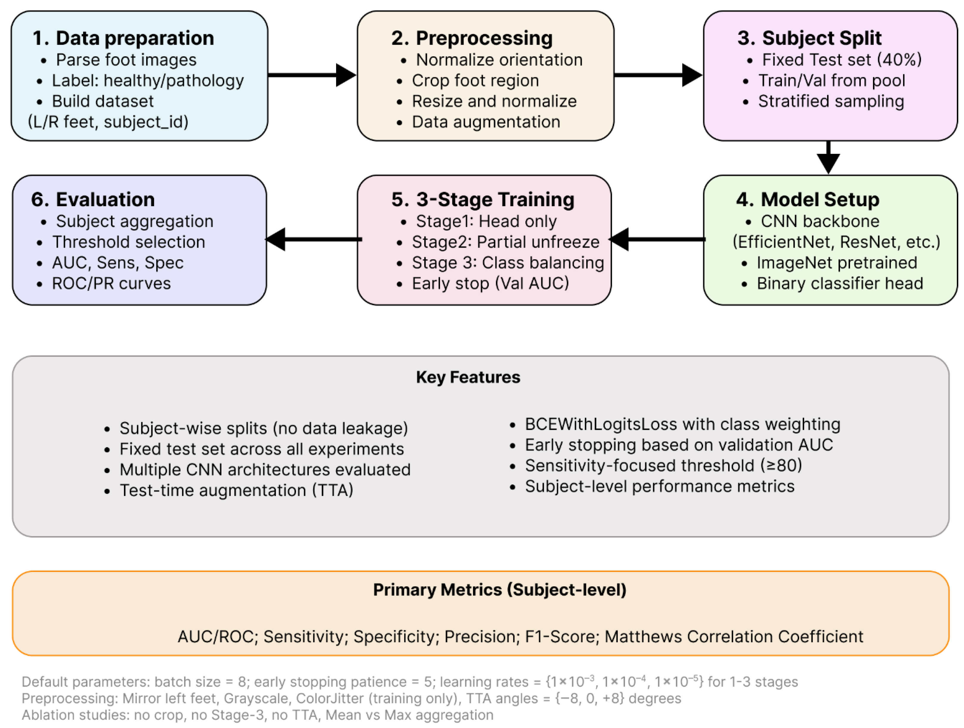
In this study (see Figure 5), the term backbone is used for the feature-extraction part of a convolutional network. The backbone receives an image and produces a compact representation, after which a single-logit classification head is applied for the binary task. All backbones were initialized with ImageNet pre-trained weights and were trained under the same three-stage schedule: the head was trained first (Stage-1), selected late backbone blocks were unfrozen and fine-tuned (Stage-2), and an optional short fine-tune with class-balance handling was performed (Stage-3). Multiple backbones were evaluated so that differences in architectural bias, capacity, and computational cost could be characterized under identical data, preprocessing, and optimization settings.

Eight families were assessed. ResNet-50 was used as a strong residual-network baseline whose stability under transfer learning has been widely observed [27]. DenseNet-121 was included to represent densely connected feature reuse, which is known to be parameter-efficient [28]. EfficientNet-B0 was chosen for its compound scaling and Mobile Inverted Bottleneck (MBConv) blocks, which frequently yield favorable accuracy-to-compute trade-offs on small datasets [29]. Two lightweight families: MobileNetV2 and MobileNetV3 (Small and Large) were included to reflect mobile/edge deployment constraints while retaining competitive transfer performance [30,31]. ConvNeXt-Tiny was used as a modern convolutional design that replaces some batch-norm/activation patterns with LayerNorm and larger effective kernels, offering transformer-like training behavior while remaining fully convolutional [32]. Two very efficient baselines, ShuffleNetV2 (×1.0) and SqueezeNet1.1, were added to probe the lower end of the parameter/FLOP spectrum [33,34]. All backbones were used only as feature extractors. The final classification layer was replaced by a single fully connected unit producing one logit.

3.2. Data Preprocessing and Standardization

In this study, the primary decision was defined at the subject level, not at the individual image level. This choice was motivated by three reasons. First, the clinical question is patient centered. In practice, management decisions are made for a subject (presence or absence of flat foot pathology), even when multiple images or both feet are available. Reporting subject-level performance therefore provides a more realistic estimate of how the system would behave in a clinical workflow. Second, subject-level aggregation reduces the risk of overly optimistic results on small datasets. If individual images from the same subject are split across training, validation, and test sets, information leakage can occur, and performance may be biased. In this study, all images from a given subject were kept strictly within a single split (train, validation, or test), and predictions from all available images of that subject were aggregated to obtain one subject-level score. Third, the computational overhead introduced by subject-level prediction is minimal. The model still operates on individual images. Subject-level output is obtained by a simple aggregation (mean or maximum) of image-wise probabilities for that subject.

Images were indexed by parsing the filename to obtain: a subject identifier, foot side, class label (healthy vs. pathology) from the enclosing folder name. To reduce nuisance variation, left feet were mirrored and (when needed) rotated to match the canonical right-foot orientation (horizontal flip and 180° rotation). A tight crop around the foot was obtained and padded to a square before resizing to the model’s input size. A tight bounding box around this component was extracted and padded to obtain a square region containing the foot. The cropped patch was then zero-padded to maintain a square aspect ratio. The padded crop was resized to the backbone-specific input size (e.g., 224 × 224 or 256 × 256 pixels) using bilinear interpolation. Pixel values were first scaled to [0, 1] and then standardized channel-wise using the ImageNet statistics (see Equation (1))

$$\begin{array}{c}{\mathit{x}}_{\mathit{c}}^{\mathit{n}\mathit{o}\mathit{r}\mathit{m}}={\displaystyle \frac{{\mathit{x}}_{\mathit{c}}-{\mathit{\mu }}_{\mathit{c}}}{{\mathit{\sigma }}_{\mathit{c}}}}, \end{array}$$

(1)

where ${\mathit{x}}_{\mathit{c}}$ is the scaled pixel intensity in channel $\mathit{c}$, and $({\mathit{\mu }}_{\mathit{c}},{\mathit{\sigma }}_{\mathit{c}})$ are the ImageNet mean and standard deviation for that channel (R: 0.485, 0.229; G:0.456, 0.224; B: 0.406, 0.225). The same normalization was applied for all backbones, matching their pretraining setup.

During training, the standardized images were further augmented with small affine transforms, brightness/contrast jitter, and occasional grayscale conversion. No augmentation was applied during validation or testing. All experiments used subject-wise splits: a single fixed test set (e.g., 40% of subjects), with train/validation drawn from the remaining pool via stratified sampling by subject. This prevents left/right images from the same person appearing in both training and evaluation.

3.3. Three-Stage Training Strategy

All models were trained with the same three-stage transfer learning strategy to ensure stable optimization on the small dataset and to make backbone comparison fair. In Stage 1, all pretrained backbone parameters were frozen and only the final classification layer (a single fully connected unit outputting one logit) was trained. This stage allowed the new head to adapt to the flat foot classification task without perturbing the pretrained feature extractor. In Stage 2, the last backbone block(s) were unfrozen (architecture-specific) together with the classification head, and joint fine-tuning was performed with a reduced learning rate. In this way, higher-level features were allowed to specialize to the target domain, while earlier layers remained regularized by the pretrained weights. In Stage 3, an optional short fine-tuning phase was performed with class-balance handling. In this stage, a weighted sampling of the minority class and, when applicable, a positive-class weighting in the loss were applied to compensate for label imbalance, while training was restricted to the same subset of parameters used in Stage 2. Early stopping based on validation performance was used in all stages to limit overfitting.

The model outputs a logit $z\in \mathbb{R}$. The predicted positive probabilities are the sigmoid:

$$\begin{array}{c}\sigma \left(z\right)={\displaystyle \frac{1}{1+e^{-z}}}. \end{array}$$

(2)

A sigmoid output was used because the task is binary, and the model was designed with a single logit. For two classes, other methods like softmax with two logits are mathematically redundant. One-logit sigmoid $\sigma \left(z\right)$ captures the same decision boundary with fewer parameters and slightly better numerical stability when paired with Binary Cross-Entropy with logits (commonly referred to as BCEWithLogitsLoss) with optional positive-class weight $w$:

$$\begin{array}{c}L\left(y,z\right)=-wy\log \sigma \left(z\right)-\left(1-y\right)\log \left(1-\sigma \left(z\right)\right), \end{array}$$

(3)

where $y\in \left\{0,1\right\}$ is the ground-truth label [35,36]. In this formulation, the network produces a single real-valued logit per image, which is internally converted to a probability by the sigmoid link while the loss is computed in a numerically stable “with-logits” form (i.e., without applying a separate sigmoid in the forward pass). This choice was made for three reasons. First, a single-logit sigmoid formulation is the minimal, standard setup for two-class problems. Second, the with-logits computation improves numerical stability by avoiding underflow/overflow that can arise when a sigmoid is applied explicitly before the cross-entropy, which is important with small datasets and class imbalance. Third, this loss supports positive-class reweighting (via a class-balance factor) so that errors on the minority class can be emphasized during optimization.

3.4. Models Setup and Evaluation

To reduce small-sample bias and quantify variability, repeated stratified subject-wise splits were used within the development set. First, a fixed test set was formed at the subject level and kept untouched for all experiments. The remaining subjects were used for training and validation. For each backbone and configuration, 10 independent train/validation splits were generated by stratified sampling on subject labels, ensuring that all images from a given subject appeared in only one subset. The model was trained and tuned on each split, evaluated on the fixed test set, and performance metrics were averaged across repeats. This repeated resampling scheme plays the role of cross-validation while preserving a single, leakage-free test set for final reporting.

The test-time augmentation (TTA) was applied consistently. Each test image was evaluated under a small set of rotations, and the resulting logits were averaged before the sigmoid function. This procedure was used to reduce prediction variance due to minor acquisition differences. In the ablation analysis, an additional “no-TTA” condition was evaluated to quantify the effect of TTA on subject-level performance. Because the decision is per subject, image-level probabilities for a subject were aggregated to a subject-level score ${\mathit{p}}_{\mathit{s}}$ by either

$$\begin{array}{c}\mathbf{mean} {\mathit{p}}_{\mathit{s}}={\displaystyle \frac{\mathbf{1}}{{\mathit{n}}_{\mathit{s}}}}{\displaystyle \sum _{\mathit{i}=1}^{{\mathit{n}}_{\mathit{s}}}}{\mathit{p}}_{\mathit{s}\mathit{i}} \mathbf{or} \mathbf{max}: {\mathit{p}}_{\mathit{s}}=\underset{\mathit{i}=1,\dots ,{\mathit{n}}_{\mathit{s}}}{\mathbf{max}}{\mathit{p}}_{\mathit{s}\mathit{i}} \end{array}$$

(4)

where ${\mathit{p}}_{\mathit{s}\mathit{i}}$ is the image-level probability for subject $\mathit{s}$ and image $\mathit{i}$; ${\mathit{n}}_{\mathit{s}}$ is the number of images for subject $\mathit{s}$. In this dataset each subject contributes two images (left and right), therefore ${\mathit{n}}_{\mathit{s}}=\mathbf{2}$ for all $\mathit{s}$ (the formula remains valid for ${\mathit{n}}_{\mathit{s}}\ge \mathbf{1}$. A subject-level decision threshold t was selected on the validation subjects using one of two rules: sensitivity-target: the smallest t such that sensitivity ≥ τ (here τ = 0.8); or Youden’s J: t maximizing $\mathit{J}=\mathit{s}\mathit{e}\mathit{n}\mathit{s}\mathit{i}\mathit{t}\mathit{i}\mathit{v}\mathit{i}\mathit{t}\mathit{y}+\mathit{s}\mathit{p}\mathit{e}\mathit{c}\mathit{i}\mathit{f}\mathit{i}\mathit{c}\mathit{i}\mathit{t}\mathit{y}-1$ [35].

The chosen threshold was then applied to the fixed test set. Primary performance was reported at the subject level. For the confusion matric entries TP, TN, FP, FN,

$$\begin{array}{c}\mathit{\text{sensitivity}}={\displaystyle \frac{\mathit{T}\mathit{P}}{\mathit{T}\mathit{P}+\mathit{F}\mathit{N}}}, \mathit{\text{specificity}}={\displaystyle \frac{\mathit{T}\mathit{N}}{\mathit{T}\mathit{N}+\mathit{F}\mathit{P}}}. \end{array}$$

(5)

AUROC, precision, F1-score, Matthews correlation coefficient (MCC), and balanced accuracy were also reported. Performance for each backbone/ablation is summarized over repeated subject-wise splits as mean ± standard deviation (std) where std reflects variability due to resampling on a small cohort.

4. Results and Discussion

4.1. Data Description and Backbone’s Comparison

In this study, a backbone is defined as the feature-extraction part of a deep network—the sequence of layers that converts an input image into a compact feature representation. The final classification layer is replaced with a single-logit head for the binary task. During Stage-1, only this head is trained; during Stage-2, the last blocks of the backbone are unfrozen and fine-tuned; during Stage-3 (optional), a short class-balance-aware fine-tune is performed.

To ensure a fair comparison, identical preprocessing and augmentation were applied across models, including orientation normalization and optional cropping/padding. Subject-wise splits were enforced to prevent leakage between training and testing. Decision thresholds were selected on the validation set to meet a target sensitivity. Performance was reported primarily at the subject level, where left/right images were aggregated (mean aggregation by default, with max aggregation examined in a secondary analysis). For each backbone, results were summarized as the mean ± standard deviation across repeated stratified splits, enabling direct comparison under matched conditions.

In Figure 6, the change in subject-level AUC (ΔAUC vs. the baseline pipeline) is shown when each major component is removed in isolation: cropping (“no_crop”), the Stage-3 class-imbalance fine-tune (“no_stage3”), and test-time augmentation (“no_tta”). A consistent negative shift is observed for “no_crop” across most backbones, with the largest drops for heavier models such as ResNet-50 and compact models such as MobileNetV3-Small. This pattern indicates that the proposed crop-and-pad normalization reduces background clutter and scale variation that otherwise degrades discrimination on small datasets. Removing TTA produces a small but recurrent decrease in AUC under mean aggregation, suggesting that averaging predictions over light rotations stabilizes scores without overfitting. The effect of disabling Stage-3 is heterogeneous: several lightweight backbones benefit noticeably from the imbalance-aware fine-tune, whereas some larger models change little or even show a slight decline, implying that the first two stages already capture most of the available signal for those architectures.

Figure 7 repeats the analysis using max aggregation at the subject level. Relative to Figure 6, the contribution of TTA becomes more backbone-dependent and occasionally turns negative, which is consistent with max pooling amplifying spurious high scores from a single view and reducing the smoothing benefit of augmentation. The penalty for removing cropping remains evident, reinforcing the importance of the proposed preprocessing canon regardless of the aggregation rule. Stage-3 again shows mixed impact, with improvements concentrated in models that exhibit greater class-imbalance sensitivity. Taken together, Figure 6 and Figure 7 support the recommended defaults for small medical image datasets: keep cropping enabled, prefer mean aggregation for stability, use light TTA by default (especially with mean aggregation), and apply Stage-3 selectively when class imbalance or backbone behavior warrants it.

4.2. Results Comparison Between Different CNN Architectures

A fixed subject-held-out test set was created once and kept unchanged for all experiments. The test set contained 40% of subjects (patient-wise split; exact counts are reported in the Dataset section). The remaining subjects formed a training/validation pool. For each backbone, models were trained in 20 independent repeats: in every repeat a new stratified subject split was drawn inside the pool to form a small validation set used for early stopping and threshold selection. Results were reported on the same fixed test set, and summary values were given as mean ± standard deviation across repeats.

Performance was computed at the subject level. Image scores for the same subject (e.g., left/right feet) were first aggregated into a single subject score using either mean or max aggregation, as specified. A decision threshold was then chosen on the validation subjects to target ≥80% sensitivity. When that target was not reachable, the Youden index (maximizing TPR–FPR) was used. Sensitivity was defined as the proportion of pathology subjects correctly flagged as positive. Specificity was defined as the proportion of healthy subjects correctly flagged as negative. “Subject accuracy” refers to the fraction of test subjects correctly classified after aggregation and thresholding.

The baseline pipeline was used: ImageNet-pretrained backbone, standardized pre-processing with cropping and padding, the proposed three-stage training schedule (head-only → partial unfreeze → class-imbalance fine-tune), mean or max aggregation at subject level, and light test-time augmentation.

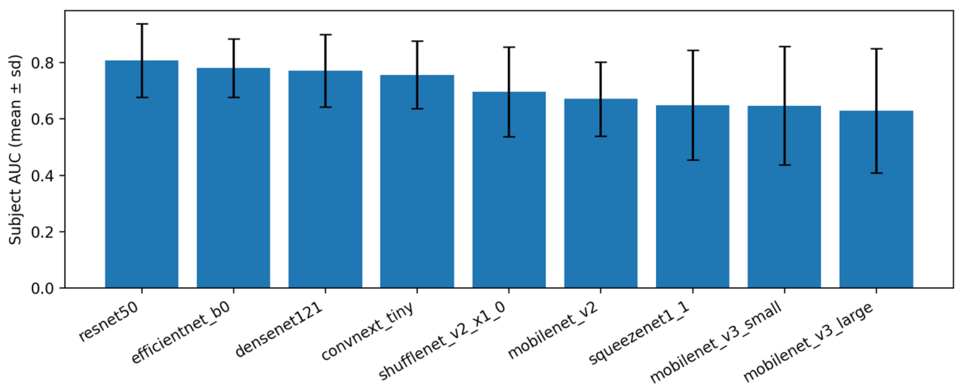
Under the proposed baseline pipeline, subject-level performance was stable across backbones when mean aggregation was used (Figure 8;

Table 2. Baseline test performance per backbone with mean aggregation (AUC, Sensitivity, Specificity, F1, and MCC values are reported as mean ± standard deviation across 20 independent runs).

Arch	Test_AUC_Subj Mean (±std)	Test_Sensitivity Mean (±std)	Test_Specificity Mean (±std)	F1_Subj Mean (±std)	MCC_Subj Mean (±std)
convnext_tiny	0.757 (±0.12)	0.45 (±0.394)	0.746 (±0.36)	0.33 (±0.249)	0.235 (±0.223)
densenet121	0.771 (±0.128)	0.55 (±0.251)	0.846 (±0.086)	0.51 (±0.207)	0.386 (±0.23)
efficientnet_b0	0.781 (±0.103)	0.475 (±0.268)	0.854 (0.16)	0.458 (±0.19)	0.372 (±0.207)
mobilenet_v2	0.671 (±0.131)	0.6 (±0.286)	0.6 (±0.323)	0.409 (±0.085)	0.212 (±0.143)
mobilenet_v3_large	0.63 (±0.221)	0.45 (±0.359)	0.738 (±0.174)	0.33 (±0.219)	0.163 (±0.229)
mobilenet_v3_small	0.647 (±0.21)	0.575 (±0.364)	0.531 (±0.201)	0.331 (±0.192)	0.088 (±0.246)
resnet50	0.808 (±0.13)	0.55 (±0.299)	0.838 (±0.277)	0.527 (±0.249)	0.439 (±0.287)
shufflenet_v2_x1_0	0.697 (±0.16)	0.575 (±0.258)	0.731 (±0.26)	0.46 (±0.203)	0.313 (±0.235)
squeezenet1_1	0.649 (±0.195)	0.525 (±0.371)	0.615 (±0.276)	0.354 (±0.262)	0.142 (±0.328)

). Across repeats, variability is shown as mean (± std) and no additional confidence intervals are reported to avoid over-interpretation on a small test cohort. The top models achieved the highest average AUROC with modest variability across repeats, while lower-capacity models trailed by a consistent margin. This pattern indicates that the pre-processing and 3-stage schedule transfer well across architectures, with differences largely attributable to backbone capacity.

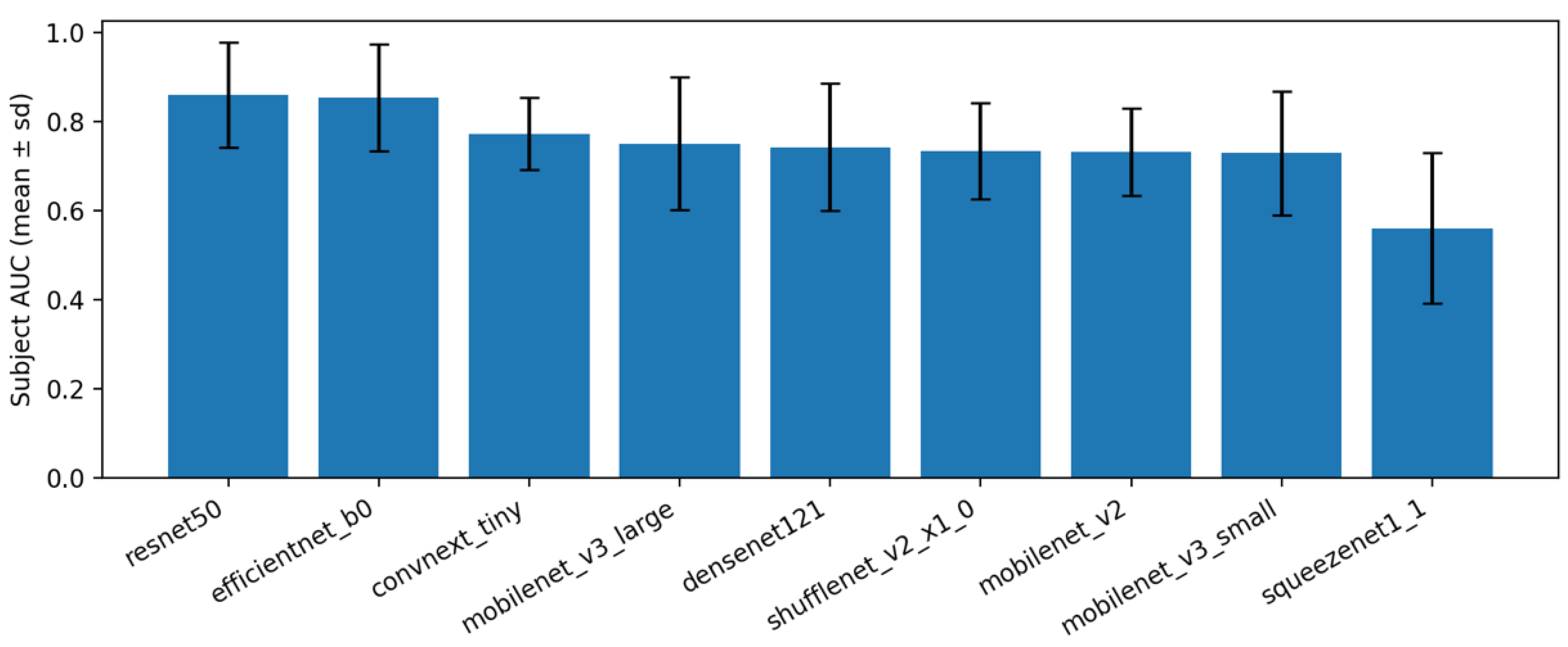
When max aggregation was applied instead of the mean (Figure 9;

Table 3. Baseline test performance per backbone with max aggregation (AUC, Sensitivity, Specificity, F1, and MCC values are reported as mean ± standard deviation across 20 independent runs).

Arch	Test_AUC_Subj Mean (±std)	Test_Sensitivity Mean (±std)	Test_Specificity Mean (±std)	F1_Subj Mean (±std)	MCC_Subj Mean (±std)
convnext_tiny	0.773 (±0.081)	0.375 (±0.401)	0.785 (±0.319)	0.264 (±0.228)	0.187 (±0.171)
densenet121	0.743 (±0.144)	0.5 (±0.363)	0.731 (±0.285)	0.38 (±0.238)	0.25 (±0.285)
efficientnet_b0	0.855 (±0.12)	0.425 (±0.345)	0.9 (±0.177)	0.428 (±0.292)	0.38 (±0.297)
mobilenet_v2	0.733 (±0.098)	0.575 (±0.305)	0.638 (±0.221)	0.383 (±0.171)	0.195 (±0.176)
mobilenet_v3_large	0.751 (±0.149)	0.5 (±0.397)	0.731 (±0.272)	0.35 (±0.256)	0.211 (±0.265)
mobilenet_v3_small	0.73 (±0.138)	0.55 (±0.276)	0.754 (±0.275)	0.471 (±0.223)	0.335 (±0.281)
resnet50	0.861 (±0.118)	0.55 (±0.299)	0.892 (±0.184)	0.571 (±0.241)	0.507 (±0.295)
shufflenet_v2_x1_0	0.735 (±0.108)	0.525 (±0.353)	0.754 (±0.261)	0.402 (±0.256)	0.269 (±0.253)
squeezenet1_1	0.562 (±0.169)	0.7 (±0.299)	0.431 (±0.341)	0.4 (±0.129)	0.126 (±0.228)

), the relative ordering of models changed only slightly and absolute AUROC values remained in a similar range. This suggests that both aggregation rules are viable on this dataset. However, mean aggregation is maintained as the default in the remainder of the work because it is less sensitive to single-view outliers and produced slightly tighter variability across repeats in most backbones.

Across repeats, the results were consistent: standard deviations around the mean subject-level AUROC were small for most backbones (Figure 8 and Figure 9; Table 2 and Table 3). Within this setting, ResNet-50 and EfficientNet-B0 achieved the highest subject-level AUROC on average, while very small networks (e.g., SqueezeNet, MobileNet-V3 Small) performed lower but still followed the same pattern across splits. These observations indicate that the three-stage training framework (head-only, partial unfreeze, imbalance-aware fine-tuning), together with orientation normalization, crop-and-pad pre-processing, and test-time augmentation, is the main source of robustness. The specific backbone mainly modulates the absolute performance level. In practice, a medium-size model such as EfficientNet-B0 offers a good accuracy (compute compromise), whereas larger models (e.g., ResNet-50) can be chosen when slightly higher accuracy is needed.

Regarding subject aggregation, max aggregation often produced slightly higher AUROC, but mean aggregation was typically more stable across repeats and gave a more balanced sensitivity–specificity profile.

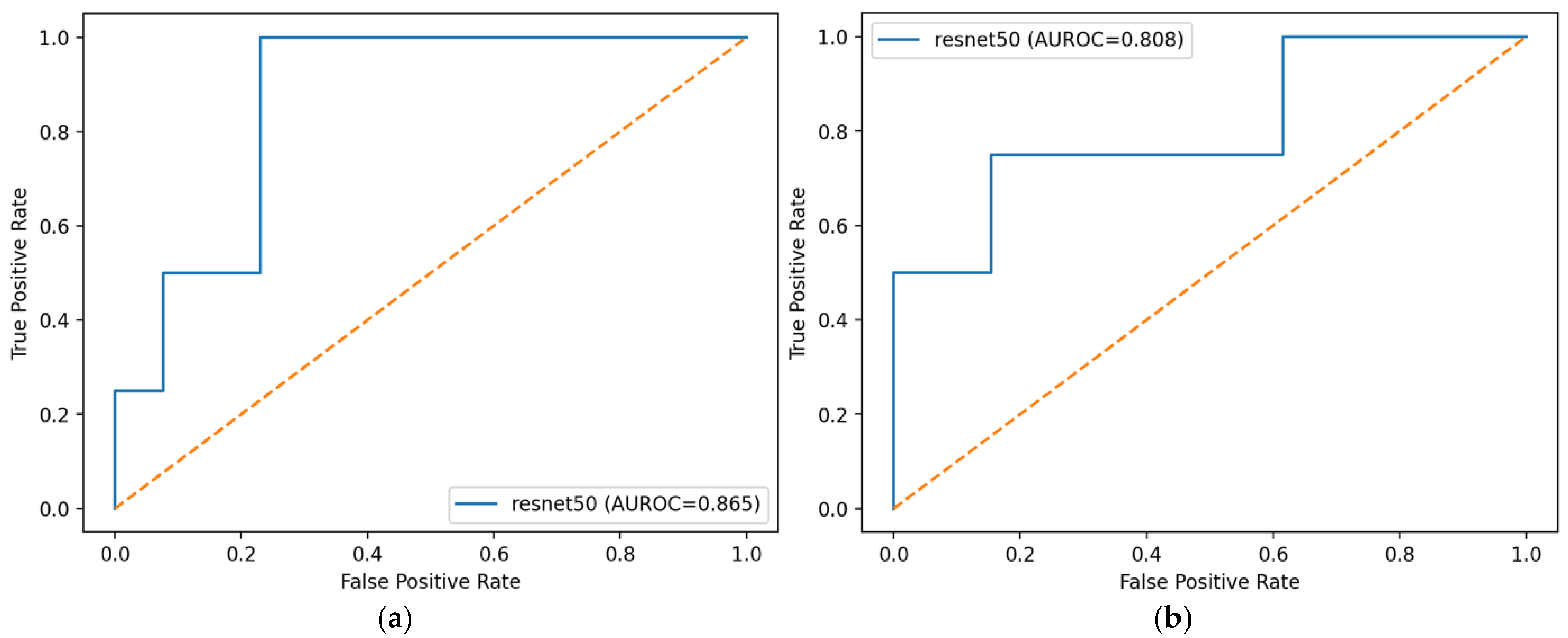
The ROC curves in Figure 10 summarize the trade-off between sensitivity and specificity at all thresholds for the selected ResNet-50 model. When subject predictions were formed by mean aggregation, the curve dominated its max aggregation counterpart and yielded a higher AUROC (0.865 vs. 0.808), consistent with the backbone comparison in Table 2 and Table 3. Mean aggregation produced a smoother profile and lower false-positive rates at comparable sensitivities, indicating greater stability across thresholds. In contrast, max aggregation amplified any single high image score within a subject, which increased the false-positive rate and reduced overall area.

The three-stage pipeline delivered stable subject-level performance across diverse ImageNet-pretrained backbones. Mean aggregation outperformed max aggregation in AUROC and variability. Cropping and TTA consistently helped, while Stage-3 imbalance tuning gave smaller, model-dependent gains. Lightweight models were competitive with larger ones, indicating the framework is effective and efficient. Overall, this leakage-aware pipeline with sensitivity-targeted thresholding is a strong, practical baseline for small medical imaging datasets.

4.3. Computational Requirements and Runtime

All experiments were conducted on a single workstation equipped with an NVIDIA T4 GPU (16 GB VRAM), an 8-core Intel Xeon-class CPU, and 16 GB RAM, using PyTorch (https://pytorch.org/) framework. For each backbone, a full 3-stage run (including training and validation) required approximately 3–6 min for lightweight models (e.g., MobileNetV3-Small, ShuffleNetV2) and 8–15 min for larger models (e.g., ResNet-50, ConvNeXt-Tiny). Inference is computationally inexpensive: for MobileNetV3-Small, a single image forward pass required well below 10 ms on GPU and below 50 ms on CPU, corresponding to real-time throughput even when subject-level decisions are based on multiple images. These measurements demonstrate that the compact backbones within the proposed pipeline are computationally feasible, while in real-world mobile or point-of-care settings the achievable latency will depend on the specific device hardware and implementation. Therefore, the reported results should be interpreted as indicative rather than device-specific guarantees.

4.4. Discussion and Limitations

The present study was conducted on a small pediatric sample (84 images out of 42 subjects, 3–14 years), which is a major limitation for both statistical power and model generalization. The reported results should therefore be interpreted as exploratory rather than definitive. In particular, the model was not explicitly stratified or adjusted for age, sex, BMI, or foot size, and it cannot be assumed that the learned decision boundary is stable across these factors. Uncertainty is expressed as the standard deviation across repeated subject-wise splits. Formal confidence intervals and hypothesis tests were not reported due to the limited cohort size, to avoid over-interpretation. The small cohort makes the results sensitive to differences in age, body mass, and foot morphology. In children, arch shape changes with growth and weight. With few subjects, a model can learn patterns that reflect this case mix rather than general features of flatfoot. No stratification or adjustment by age, BMI, or foot size was performed, and no normalization for these factors was applied. Therefore, the reported metrics should be read as conditional on this cohort.

Below is a

Table 4. Quantitative summary of related AI/baropodometric approaches.

Modality	Population	Ground-Truth/Labeling	Model/Approach	Primary Metrics (as Reported)	Notes/Limitations
Plantar pressure (baropodometry) [37]	Mixed population (clinical outpatients); N adolescent cohort (paper proposes dataset & DL baseline)	Expert labeling of foot type from pressure maps	CNNs on pressure images (baseline architectures); demo pipelines for screening feasibility	Reports classification results (accuracy/sensitivity/specificity) on internal splits; aimed at screening feasibility	Adolescent cohort; single-center; dataset specifics and generalizability discussed
Smartphone photographs (multi-view foot photos) [19]	Mixed population (clinical outpatients); N reported in study	Orthopedic diagnosis (pes planus/normal/cavus) based on clinical exam	CNN classifier trained on smartphone images; mobile-friendly workflow	AUROC/accuracy reported for pes planus vs. other classes on internal test	Real-world photos; illumination/pose variability; single-center
Footprints (RGB images) [38]	Mixed population (clinical outpatients); N in study; curated footprint photos	Foot-type labels (flat/normal/high arch) assigned by clinicians	CNN on footprint RGB with augmentation; comparison to classic indices	Accuracy/F1 across classes on held-out set	Non-clinical capture settings; external validation pending
Radiographs (weight-bearing foot X-rays) [39]	Adults; N labeled radiographs	Radiologist labels for pes planus vs. normal	Transfer learning on standard CNNs (e.g., ResNet/EfficientNet variants)	AUROC/accuracy for pes planus detection; ablation on TL setups	Single-modality X-ray; adult cohort; generalizability to pediatrics not established
Wearable plantar sensors (pressure time-series) [40]	Mixed population (clinical outpatients); N footwear-sensor recordings	Foot-type labels from clinical assessment	1D-CNN on pressure time-series	Accuracy on cross-validation	Wearable context; differs from static plate; deployment angle is mobile

that provides a quantitative summary of the related artificial intelligence and baropodometric methods.

Future work should include multi-center datasets with broader demographic and anthropometric coverage. Also, an adult classification framework may not be appropriate for this cohort, and the current model targets only binary detection (healthy vs. flatfoot) rather than calibrated pediatric staging. The binary labels were derived from routine clinical judgment rather than a standardized pediatric flatfoot index (e.g., PTT). This may limit comparability with other cohorts and underlines the need to harmonize labeling criteria in future work.

No direct numerical comparison with previous AI-based or baropodometric flatfoot assessment studies was performed. Existing approaches differ in acquisition modality (e.g., footprint ink, pressure plates, radiographs, photographs), labeling protocols, and target populations, which makes a pooled performance ranking difficult to interpret. Instead, this study focuses on providing a transparent, reproducible pipeline for small datasets with strict subject-wise separation and well-defined evaluation. The proposed framework is intended to complement, rather than replace, existing methods, and can be applied to other modalities when appropriate data is available.

Although the current implementation addresses a binary decision (flatfoot vs. non-flatfoot), the underlying architecture can be extended to multi-class or ordinal classification of severity stages by replacing the single-logit head with multiple outputs or an ordinal regression formulation. However, such extensions would require reliably annotated data for each stage, careful handling of class imbalance, and evaluation tailored to ordered categories. As no such dataset was available in this work, the multi-stage scenario is left as future work.

From a clinical perspective, the proposed system is best viewed as a decision-support tool for pediatric orthopedics, not as a standalone diagnostic. The workflow assumes standardized acquisition of images or scans, automated preprocessing, and subject-level prediction that can assist clinicians in triage or follow-up. Lightweight backbones included in this study suggest that deployment on low-cost hardware or mobile devices is technically feasible, but this will depend on actual device specifications, software optimization, and regulatory validation. Community or school screening using mobile cameras or affordable 3D/pressure devices is therefore a realistic long-term direction but requires prospective validation studies before routine use.

5. Conclusions

This study presents a methodology based on the application of artificial intelligence tools to detect flatfoot pathology in children. Measured 3D images were taken that reflect the structure of the patient’s foot. The observations made showed that the proposed three-stage training system, together with orientation normalization, cropping and dilation pre-processing, and test time padding, is the main source of reliability. The specific backbone mainly modulates the absolute performance level. Using 8 different models and training them 20 times, after applying the proposed model improvements, it is possible to assess the presence/absence of flatfoot pathology in children. Regarding the aggregation of subjects, the maximum aggregation often gave a slightly higher AUROC, but the average aggregation was generally more stable between repetitions and gave a more balanced sensitivity and specificity profile.

Our study and the proposed methodologies showed the best accuracy with two architectures—resnet50 and efficientnet_b0, which have accuracies of 0.808 (±0.13) and 0.781 (±0.103) when the average aggregation value is, and 0.861 (±0.118) and 0.855 (±0.12) when the maximum aggregation value of the study level is.

In the future, we plan to apply this method to determine the stages of flatfoot pathology described in this article. This is a new and complex process, but in the field of orthopedics it would help to determine the stage of pathology faster and more accurately.