Multi-Criteria Framework for Evaluating Robotic Arm Power Prediction Models

Abstract

As the use of industrial robotic arms (RAs) increases, effective energy management has become a critical requirement for manufacturing competitiveness and sustainability. However, existing power prediction models are often based on complex kinematic or dynamic formulations, limiting their applicability on the shop floor. To address this challenge, this study develops an evaluation framework for regression-based RA power prediction models that integrates accuracy, explainability, and practical considerations. Specifically, 162 statistical and machine-learning models are evaluated in terms of model type, movement type, training data size, and training time. The results show that the support vector machine (SVM) consistently outperforms other models in both accuracy and computational efficiency, while the multilayer perceptron (MLP) performs the worst. Using Shapley additive explanations (SHAP), the framework also clarifies how the most effective models capture the physical characteristics of RA movements embedded in power data. Moreover, the analysis reveals that similar movement patterns, such as along the X and Y axes, can result in distinct power demands. These findings highlight the need for explainable and practical prediction models to support energy-efficient RA operations and provide shop-floor engineers with actionable insights into the physical mechanisms driving power demand.

1. Introduction

In the manufacturing process, industrial robots play a key role in improving productivity, flexibility, and cost efficiency [1]. The importance of industrial robots in shop-floor manufacturing is also reflected in recent studies on robotic-cell operations and system-level optimization [2,3]. Among various industrial robots, robotic arms (RAs) are particularly one of the most widely used types, representing over 40% of the industrial robot market [4]. As the use of industrial robots expands, energy consumption by industrial robots is also increasing [5,6]. The energy consumption of industrial RAs is tightly connected to a manufacturer’s environmental impact, production costs, and competitiveness [7,8,9]. Thus, effectively managing the energy consumption of RA is significantly important. Nonetheless, major initiatives to enhance the energy efficiency of RA remain limited. Energy is often wasted in practice because shop-floor engineers typically have little access to information or knowledge on the energy consumption of RAs [10]. Therefore, to manage the energy efficiency of RAs, decision support tools that can help shop-floor engineers understand how RA operations drive energy consumption need to be introduced.

Specifically, two primary characteristics are required for an effective decision support tool to support shop-floor engineers in improving the energy efficiency of RAs. The first characteristic is the capability to readily and accurately predict the power required for each RA operation [11,12]. Although several models have been developed to predict the power demand of RAs, most are based on complex kinematics and dynamics formulations [13]. These models require an excessive number of mechanical inputs and therefore have limited applicability on the shop floor [14]. Accordingly, manufacturing shop floors require simplified regression approaches that utilize simply obtainable data such as RA movement’s coordinates and path lengths [14]. Thus, intuitive statistical or basic machine-learning (ML) models are especially promising. Then, a careful comparison is also necessary to identify the most useful RA power prediction model.

The second characteristic is the ability to help shop-floor engineers readily identify which physical or operational factors influence RAs’ power demand. In this context, while evaluating and comparing prediction models by accuracy is important, accuracy alone rarely ensures practicality on the shop floor. More specifically, the high accuracy of power prediction alone is not sufficient to connect an engineer’s hands-on experience to actual energy savings. Thus, if attention is confined only to accuracy, engineers would struggle to gain intuitive insights for system improvement [15]. However, research studies that directly connect this field experience to energy-saving outcomes are insufficient. Therefore, evaluating the prediction model’s explainability (i.e., the ability to link the physics of RA operations to power demand) is highly beneficial [16]. For that, the following two approaches can be employed: (i) explainable AI (XAI) technique and (ii) comparative analysis on regression models with multiple factors.

XAI can provide explainability of the RA power prediction model. More specifically, XAI can clarify how the physical operation of motor-driven joints is embedded in data and represented in power prediction outcomes. This perspective can offer practitioners context-based guidance for model selection under real operating conditions [16].

As for prediction model comparison, treating the type of RA’s movement as a factor can help shop-floor engineers select the most useful model for a given task. Moreover, the model’s sensitivity to the training data size (e.g., with different proportions of the available data) needs to be considered because data collection is often constrained in industry [17]. Similarly, training time can also be a critical consideration on the shop floor [17]. Accordingly, a decision support tool has to be developed to integrate the multiple considerations and their trade-offs, enabling engineers to predict and manage the energy consumption of RA better.

Taken together, effectively managing the energy consumption of RA on the shop floor requires models to offer both high predictive accuracy and applicability, as well as a clear explanation of how physical motions drive power demand. Most existing approaches are complex kinematics- or dynamics-based formulations with limited practical usability. This study addresses the limitations of prior research and makes three main contributions as follows. First, we present an accessible, regression-based power prediction model that practitioners can readily understand and apply. Specifically, we collect and utilize the data of RAs with seven degrees of freedom (7-DOF), the most commonly utilized robots in manufacturing [18,19]. Second, our evaluation framework compares multiple RA power prediction models not only by accuracy but also with respect to operational context, training data size, and training time. Accordingly, the main goal of this study is the development of a multi-criteria comparison framework that systematically evaluates RA power prediction models across the four key evaluation dimensions. Third, coupled with XAI analyses, this framework provides actionable, ready-to-follow guidelines for energy-efficient operation in manufacturing. In particular, we incorporate Shapley additive explanations (SHAP) as XAI analyses to assess whether each model accurately captures the physical dynamics underlying RA power consumption. This interpretability bridges the gap between prediction performance and practical applicability on the shop floor. The remainder of this paper is organized as follows. Section 2 reviews previous studies on energy and power prediction models and on comparisons between statistical and ML approaches. Section 3 describes the data used in this study and the methodologies employed within the proposed comparison framework. Section 4 presents the comparison results and the corresponding discussions, and Section 5 discusses the contributions of this study and outlines future research directions.

2. Literature Review

To reduce and manage the energy consumption of industrial robots, accurate power prediction models are essential [20]. For this reason, several previous studies have suggested power prediction models of RAs. Previous studies on power prediction for RAs largely fall into two categories: kinematics- and dynamics-based formulations and simplified data-driven models.

Most kinematics- or dynamics-based studies relied heavily on complex physics. Mahdavian et al. [21] suggested a model based on inverse kinematics and inverse dynamics, considering various physical parameters. Similarly, Mohammad et al. [22] developed a power prediction model of the 4-DOF RA with kinematic equations and an explicit dynamics model. These kinematics- and dynamics-based methods generally require an excessive number of mechanical inputs (e.g., RA’s position, joint angles, payload, velocities, and accelerations) and advanced expertise. Thus, these models are inappropriate to be simply and directly adopted on the shop floor.

Contrary to physics-based methods, several studies presented simplified, data-driven approaches based on statistics or ML. These approaches are more acceptable for industrial applications. As an example of a statistics-based model, Chemnitz et al. [23] predicted the power of RAs through polynomial approximation. Garcia et al. [24] proposed a RA power prediction model based on the design of experiments (DOE) and analysis of variance (ANOVA). Similarly, Guerra-Zubiaga and Luong [25] suggested an ANOVA-based power prediction model considering RAs’ speed, acceleration, payload, and temperature as operating parameters. However, these statistics-based models are often restricted in their capacity to capture the complex patterns of real-world data. In contrast, ML-based models (e.g., those including angular velocity, payload, and movement types) achieved high accuracy of predictions [26,27,28].

A critical trade-off exists in selecting between statistical and ML models for the shop-floor application. Statistical models are highly interpretable and quick to train. ML models offer superior accuracy but typically demand more complex parameter settings and a longer training time. Furthermore, one of the significant constraints in real-world manufacturing is data scarcity: the quantity of training data can significantly limit the feasibility of complex, data-dependent ML models [17]. Thus, selecting a suitable model for the shop floor requires navigating this complex trade-off among accuracy, training data size, training time, and interpretability.

Nevertheless, most studies on the RA power prediction have limited their scope. Some studies have focused solely on evaluating the accuracy of individual models [23,24,25], while others have simply compared accuracy without considering the underlying physical factors [26,28]. This narrow focus on accuracy is a fundamental research gap; if the only accuracy is considered, shop-floor engineers cannot get the intuitive, context-based insights needed to effectively reduce the energy consumption of RA [15]. Several previous studies in various fields have compared the performance of statistical and ML models, as summarized in

Table 1. Summary of previous studies comparing statistical and ML models.

Reference	Model		Performance Metric
	Statistical	ML
[29]	LR	RF, SVM, GB	R2, RMSE
[30]	LR, Logistic regression, Ridge regression, LASSO regression, SMR, PR, ENET	DNN, DT, Classifier, XGBoost	RMSE
[31]	LR	SVM, DT, RF	R2, MSE, RMSE, MSLE
[32]	PR	ANN	R2, NRMSE, percentage error
[33]	LR	RF	R, RMSE
[34]	LR, PR	ANN	R, RMSE, MAE, MAPE
[35]	LR, Ridge regression, Nonlinear regression	ANN, RF	R2, RMSE, MAE, MAPE
[36]	GLM, ENET, MARS	RF	R2, RMSE
[37]	LR, Ridge regression, LASSO regression, SMR, GLM, ENET, Cubist	ANN, RF	R2, RMSE

[29,30,31,32,33,34,35,36,37]. As statistical models, previous studies adopted various models such as linear regression (LR), logistic regression, ridge regression, least absolute shrinkage and selection operator (LASSO) regression, stepwise multiple regression (SMR), generalized linear model (GLM), nonlinear regression, polynomial regression (PR), elastic net (ENET), multivariate adaptive regression splines (MARS), and Cubist. As ML models, previous studies adopted various models such as artificial neural network (ANN), deep neural network (DNN), support vector machine (SVM), decision tree (DT), random forest (RF), classifier, gradient boosting (GB), and XGBoost. As comparison metrics, R², correlation coefficient (R), root mean squared error (RMSE), mean squared error (MSE), mean squared logarithmic error (MSLE), normalized root mean squared error (NRMSE), mean absolute error (MAE), percentage error, and mean absolute percentage error (MAPE) were used. Especially, R² is the most widely used metric. While R² is useful, it is not ideal for comparing linear and nonlinear models and can be misleading due to overfitting [38]. Therefore, metrics that directly measure prediction errors, such as RMSE or MAPE, are more appropriate. However, these previous studies solely focus on accuracy and show the absence of a comprehensive framework. Such a framework would need to simultaneously consider predictive accuracy, operational context, training data size, and model explainability.

To bridge the research gap, a new evaluation framework needs to be developed for RA power prediction models. This framework should be able to incorporate the interpretation of prediction models based on physical features. Notably, XAI can be useful to clarify how the model links RA’s physical operation (e.g., gravity-related displacement) to power demand, instead of relying solely on statistical goodness-of-fit [16]. To enable this systematic comparison and deliver practical guidance, we propose a multi-criteria comparison framework. First, our framework begins with comprehensively evaluating the accuracy of RA power prediction models. Specifically, we analyze how the power prediction results are influenced by three key factors (model type, operational context, and training data size). Here, GLM is employed as a statistical tool to analyze the effects of various factors on prediction accuracy. GLM is widely used for analyzing the effects of multiple independent variables on a dependent variable by estimating the coefficients of independent variables or by conducting ANOVA [39]. Accordingly, we develop a GLM with MAPE as a dependent variable and the levels of three factors as independent variables. We then employ trade-off analysis to supplement accuracy-focused analysis and incorporate a critical real-world constraint. In manufacturing, model training time is a crucial practical constraint [17]. We therefore analyze the trade-off between MAPE and training time using Pareto frontier analysis, a method that visualizes the optimal balance between two competing objectives [40].

As the final and most critical step, we integrate SHAP analysis to provide the intuitive and insightful XAI. SHAP is a widely used XAI method that quantifies feature contributions to predictions using Shapley values from game theory [41]. In a SHAP plot, features are listed in descending order of importance, and the SHAP value quantifies the influence of each feature on the predicted outcome [42]. In addition, the data points of each feature are displayed in different colors according to their values; the more evenly the color spectrum is aligned, the more linear the relationship between the feature and the prediction [43]. Through this SHAP analysis, it is possible to assess how well each prediction model reflects the characteristics of the features. By quantifying and visualizing the feature contribution, SHAP allows us to assess whether a model’s performance is rooted in an understanding of the RA’s physical operation. More specifically, to refine our SHAP analysis, we also conduct an empirical validation of the RA’s joint movements. In this way, our proposed framework’s core contribution is to enable the selection of an accurate, useful, and explainable RA power prediction model.

In summary, while existing research studies offer various power prediction models for RAs, they are inappropriate for simple adoption on the manufacturing shop floor. Moreover, previous studies on prediction model comparison are limited by their focus on prediction accuracy alone and inadequate comparison metrics. Therefore, to bridge this research gap, this study establishes a multi-criteria comparison framework to evaluate various statistics- and ML-based RA power prediction models. Through this systematic framework, we aim to provide clear, actionable guidance for energy management on the shop floor.

3. Data and Methodology

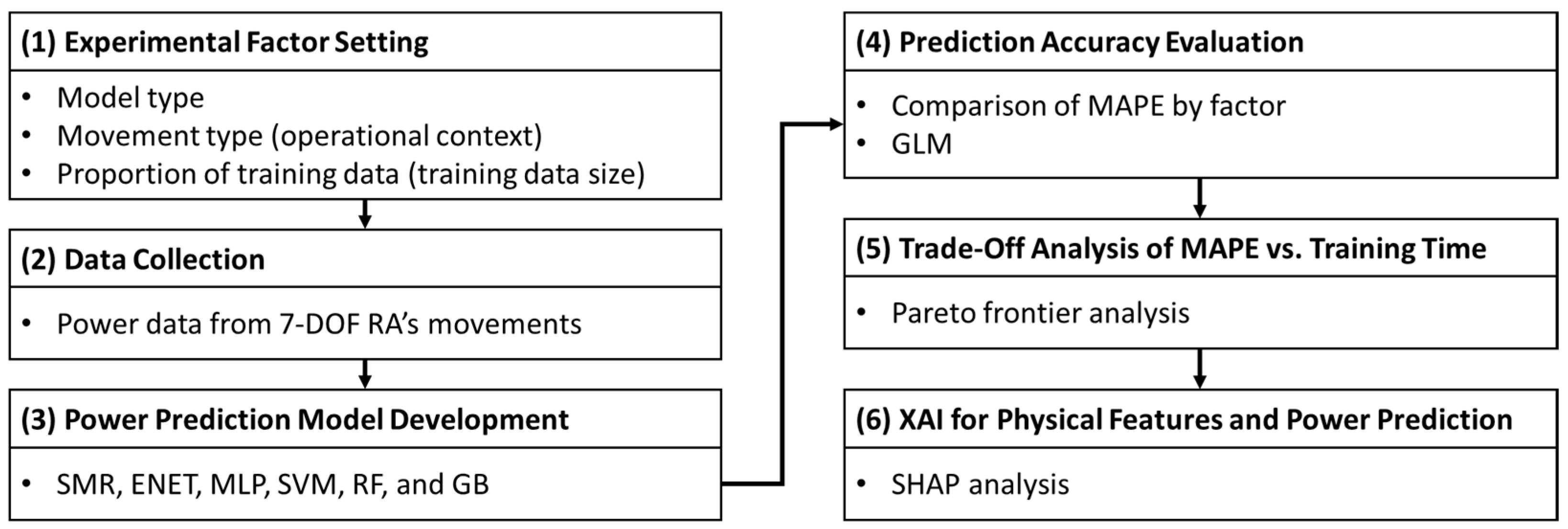
Our overall approach is outlined in Figure 1. At the first step, we set experimental factors: model type, operational context, and training data size. More specifically, as an operational context factor, the type of RA’s movement is considered, and as a training data size factor, we adopt the proportion of training data. Next, we collect power data from the movement experiment of a 7-DOF RA. Then, we develop RA power prediction models based on six model types (SMR, ENET, multilayer perceptron (MLP), SVM, RF, and GB models). These model types have been widely adopted and have shown good performance in previous studies (in Table 1), and so they are considered in this study. In particular, we employ an MLP model as the representative ANN, because most ANN models adopted in prior studies are implemented as MLP architectures with one or more hidden layers [32,34,35,37]. For the next step, we evaluate the models’ predictive accuracy (i.e., MAPE) by three factors and adopt GLM to statistically validate the influence of each factor. Additionally, we complement the accuracy evaluation with a Pareto frontier analysis to identify the most efficient models, considering training time, in terms of practicality. Lastly, we conduct SHAP analysis on the best and worst performing models found by the Pareto frontier analysis to explain how they reflect physical features in their predictions.

This section explains the experimental factors set for the comparison of RA power prediction models. This section also describes the process of power data collection of various movements of the RA. In addition, statistics and ML-based prediction model developments are introduced with their configured hyperparameters. Moreover, we describe how we build the GLM for analyzing the influence of each factor.

3.1. Experimental Factor Setting

To compare the performances of RA power prediction models by operational context and the training data size, we set experimental factors as shown in

Table 2. Experimental factors and levels for the RA power prediction model comparison.

Factor	Level
Model type	SMR, ENET, MLP, SVM, RF, GB
Movement type (operational context)	1D, 2D, 3D
Proportion of training data (training data size)	10%, 20%, 30%, 40%, 50%, 60%, 70%, 80%, 90%

. The first factor is a model type; we consider two statistics-based models (SMR and ENET) and four ML-based models (MLP, SVM, RF, and GB). As a factor for operational contexts, we adopt the movement type of RA. There are three levels for the movement type factor: one-dimensional (1D), two-dimensional (2D), and three-dimensional (3D) movements. We describe RA’s movements with the coordinates of the end effector. These coordinates are defined as the center of the flange, a circular plate-like component at the tip of the arm [14]. Also, all numbers in coordinates are set in meters. In 1D movements, only one coordinate value (X, Y, or Z) changes, creating a linear path parallel to that specific axis (e.g., moving from (0, 0, 0) to (2, 0, 0)). In 2D movements, two coordinate values change simultaneously, creating a diagonal path across a plane (e.g., the XY, YZ, or XZ plane). For instance, a 2D movement from (0, 0, 0) to (2, 2, 0) follows a direct diagonal line. In 3D movements, all three coordinate values change simultaneously, resulting in a diagonal path through three-dimensional space (e.g., moving from (0, 0, 0) to (2, 2, 2)). The last factor is the proportion of training data, which is regarded as the training data size factor. Because the model’s prediction performance can vary depending on the amount of training data, we set nine levels for the proportion of data used for training, ranging from 10% to 90% in intervals of 10%. The remaining data not used for training is entirely used as test data.

3.2. Data Collection

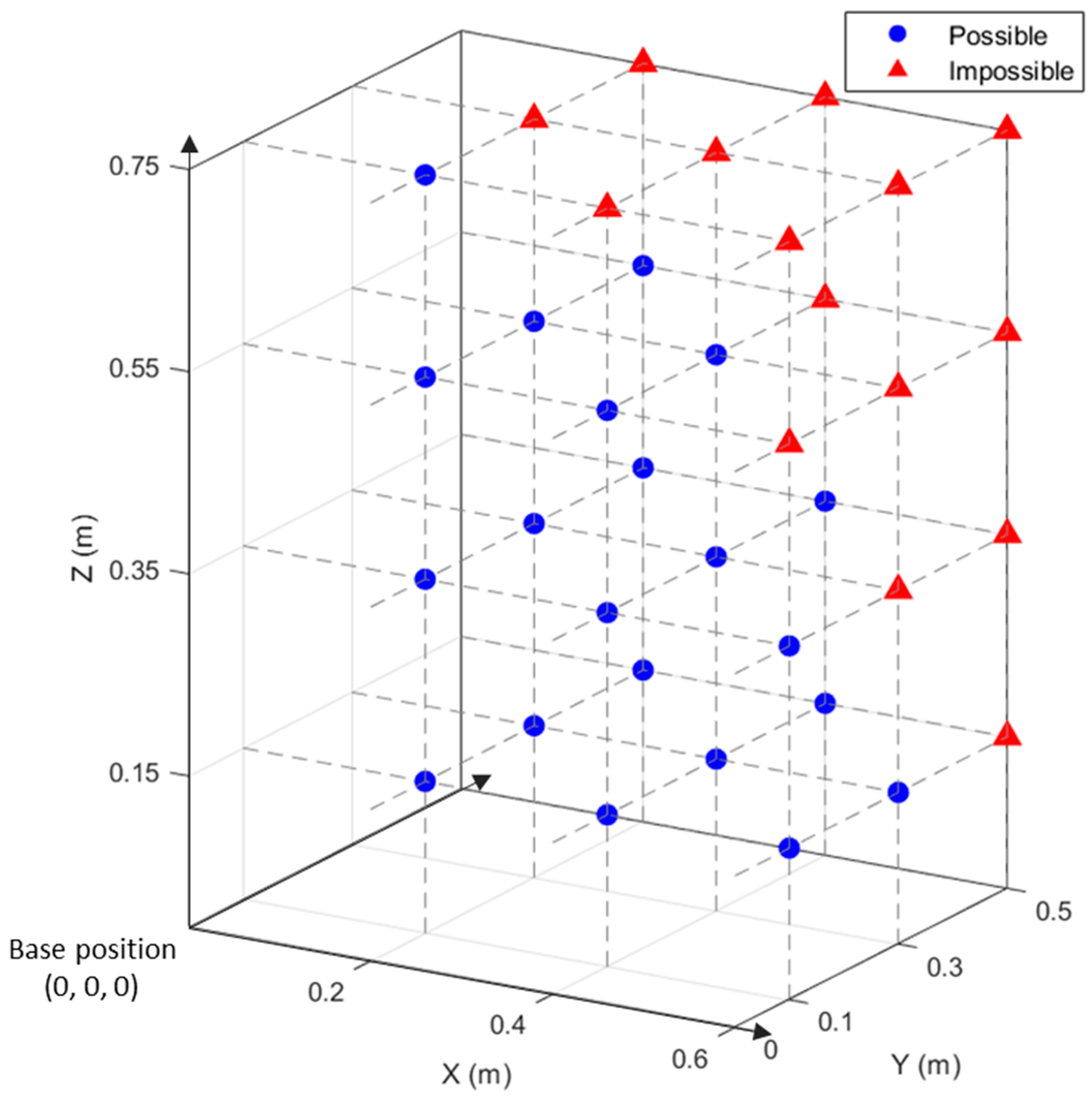
We collect the power data of a 7-DOF RA to develop and compare the power prediction models. The utilized equipment is the Ufactory xArm 7 (UFACTORY US, New York, NY, USA) with a maximum travel speed of 1 m/s and a maximum reach of 0.7 m [44]. The coordinate of the base position (i.e., the location where the RA’s base is fixed to the ground) is set as (0, 0, 0). The RA has a reach of 0.7 m, and its end effector can move within a spherical workspace centered at (0, 0, 0.12 m). Figure 2 shows the possible coordinates for the end effector’s starting and ending points. We set a grid of coordinates by defining points at 0.2 m intervals within the movement range of each axis: X [0.2, 0.6 m], Y [0.1, 0.5 m], and Z [0.15, 0.75 m]. Within this range, there are 3 discrete points on the X and Y axes, and 4 on the Z-axis. Thus, a total of 36 coordinate combinations (3 × 3 × 4) are theoretically possible. However, due to the maximum reach of the RA, only 21 coordinates are actually reachable (Figure 2). These 21 coordinates can be either the starting point (X₀, Y₀, Z₀) or the ending point (X₁, Y₁, Z₁) of the RA’s movement. Thus, the number of possible combinations of the starting and ending points is 420 (₂₁P₂).

The power of the RA’s movements, from the starting point to the ending point, is measured by a power meter (Fluke 1732 [45]) directly connected to the RA. In addition, the velocity of the RA is fixed at 0.1 m/s, and the acceleration is fixed at 2 m/s². We collect power data at 1-s intervals for each movement, and the averaged values are employed for each movement. According to the experimental range setting, we collect power data on all 420 movement cases with five replications, resulting in a total of 2100 observations.

3.3. Power Prediction Model Development

We utilize two statistics-based (SMR and ENET) and four ML-based (MLP, SVM, RF, and GB) model types to develop RA power prediction models. In prediction models, the X, Y, and Z-coordinates of the starting and ending points of the RA’s end effector (i.e., X₀, Y₀, Z₀, X₁, Y₁, and Z₁) are used as input features. In addition, the average power values of each movement (collected following the procedure outlined in Section 3.1) are used as output features. A distinct model is constructed for every possible combination of the experimental factor levels presented in Table 2, resulting in 162 (6 × 3 × 9) models in total. Equivalently, 27 models are developed for each of a total of the six model types. To enhance the performance of both statistical and ML models, we tune hyperparameters for all 162 individual models by comparing their MSE values, referring to previous studies on statistical and ML model developments [46,47]. All tuning and performance evaluation procedures employ 5-fold cross-validation. For model development and training, Intel^® Core™ i5-12600K (Intel Corporation, Santa Clara, CA, USA) and the Scikit-learn library (version 1.6.1) are used.

3.3.1. Statistics-Based Power Prediction Models

We adopt SMR and ENET as statistics-based models. SMR is a statistical algorithm used to automatically select the best subset of independent variables to improve the performance of the regression model [39]. There are two main types of variable selection: forward selection and backward elimination. SMR evaluates various statistical criteria, such as t-statistics, F-statistics, MSE, and RMSE, for adding or removing variables [39,48]. In this study, in addition to linear terms of input features (i.e., X₀, Y₀, Z₀, X₁, Y₁, and Z₁), quadratic terms and interaction terms are included in the pool of potential independent variables. A total of 27 SMR models constructed for all combinations of the levels of movement and proportion of training data are presented in

Table A1. Selection type and the number of selected terms of SMR by experimental factors.

Experimental Factor		Selection Type	The Number of Selected Independent Variables	MSE
Movement Type	Proportion of Training Data
1D	10%	Forward	14	79.13
	20%	Forward	14	71.69
	30%	Backward	14	14.28
	40%	Backward	14	8.22
	50%	Forward	14	7.74
	60%	Forward	14	5.37
	70%	Forward	14	3.61
	80%	Forward	14	4.14
	90%	Backward	14	3.86
2D	10%	Forward	14	34.29
	20%	Forward	14	9.23
	30%	Forward	14	5.38
	40%	Backward	14	4.58
	50%	Backward	14	2.88
	60%	Backward	14	2.82
	70%	Forward	14	2.80
	80%	Backward	14	2.77
	90%	Backward	14	3.07
3D	10%	Forward	14	33.96
	20%	Forward	14	18.02
	30%	Forward	14	8.54
	40%	Forward	14	5.26
	50%	Forward	14	3.28
	60%	Forward	14	3.04
	70%	Forward	14	3.52
	80%	Forward	14	3.04
	90%	Backward	14	3.05

of Appendix A.

ENET is a regularized regression method that addresses the limitations of LASSO and Ridge regression in variable selection. LASSO is strictly convex, but it sets the coefficients of unimportant variables to zero, which can create issues when there are highly correlated independent variables, as some variables can be removed [49]. In contrast, Ridge regression is not strictly convex, so it may not yield a unique solution [50]. ENET combines the strengths of both LASSO and Ridge, maintaining strict convex edges while considering the group properties of variables [51]. In ENET, two hyperparameters need to be tuned: $\lambda$ and $\alpha$. $\lambda$ controls the overall strength of the regularization and takes a value of $\lambda \ge 0.$ As $\lambda$ increases, the size of the regression coefficient decreases, reducing the complexity of the model. $\alpha$ balances the contribution of L1 (LASSO) and L2 (Ridge) penalties and takes a value between 0 and 1. When $\alpha$ is close to 0, the model is close to Ridge regression, while when $\alpha$ is close to 1, it is close to LASSO regression. The hyperparameter candidates of ENET are presented in

Table 3. Hyperparameter candidates of ENET.

Hyperparameter	Candidate
$\lambda$	0.01, 0.1, 1, 10, 100
$\alpha$	0, 0.1, 0.2, 0.3, 0.4, 0.5, 0.6, 0.7, 0.8, 0.9, 1.0

, and selected hyperparameters for each level of 27 ENET models are presented in

Table A2. Selected hyperparameters of ENET by experimental factors.

Experimental Factor		Hyperparameter		MSE
Movement Type	Proportion of Training Data	$\mathit{\lambda }$	$\mathit{\alpha }$
1D	10%	1	0.6	24.52
	20%	0.01	0.1	247.47
	30%	0.1	0	15.87
	40%	0.1	0	10.58
	50%	0.1	0	8.51
	60%	0.1	0	8.34
	70%	0.1	0	5.05
	80%	0.1	0	5.79
	90%	0.1	0	5.12
2D	10%	10	0.3	70.54
	20%	0.01	0	24.86
	30%	0.1	0	7.09
	40%	0.1	0	4.55
	50%	0.1	0	2.86
	60%	0.1	0	2.64
	70%	0.1	0	2.63
	80%	0.1	0	2.35
	90%	0.1	0	2.66
3D	10%	1	0.1	15.44
	20%	0.01	0	57.10
	30%	0.01	0	8.17
	40%	0.1	0	6.71
	50%	0.01	0.3	3.23
	60%	0.01	0.6	3.02
	70%	0.1	0	3.55
	80%	0.01	0	2.80
	90%	0.01	0.4	2.45

of Appendix A.

3.3.2. ML-Based Power Prediction Models

We adopt MLP, SVM, RF, and GB as ML-based model types. MLP is suggested to supplement a single-layer perceptron (SLP) by adding hidden layers between the input and output layers [52]. There are several hyperparameters to determine for developing the MLP model: the number of hidden layers, the number of neurons in each hidden layer, the activation function, and the learning rate [46]. To tune these hyperparameters, we set the candidates as shown in

Table 4. Hyperparameter candidates of MLP.

Hyperparameter	Candidate
Hidden layer sizes	(64, 32), (256, 128), (512, 256), (64, 32, 16), (256, 128, 64), (512, 256, 128)
Activation function	Tanh, ReLU
Learning rate	0.01, 0.001, 0.0001

and compare the MSE of all combinations of them. Two hyperparameters, the number of hidden layers and the number of neurons in each hidden layer, are considered together as ‘hidden layer sizes’ in Table 4. Referring to the previous studies, we consider two or three layers, and each layer can consist of 16, 32, 64, 128, 256, or 512 neurons [53,54]. For activation functions, we consider hyperbolic tangent (tanh) and rectified linear unit (ReLU) functions because they are the most widely used activation functions [55]. For candidates of the learning rate, a hyperparameter determines the step size for updating weights; we include 0.01, 0.001, and 0.0001 [56]. The hyperparameters selected for 27 models are shown in

Table A3. Selected hyperparameters of MLP by experimental factors.

Experimental Factor		Hyperparameter			MSE
Movement Type	Proportion of Training Data	Hidden Layer Sizes	Activation Function	Learning Rate
1D	10%	(64, 32, 16)	ReLU	0.001	568.53
	20%	(512, 256)	ReLU	0.001	219.60
	30%	(256, 128, 64)	ReLU	0.001	324.28
	40%	(512, 256, 128)	ReLU	0.001	265.97
	50%	(512, 256)	Tanh	0.001	19.27
	60%	(512, 256, 128)	ReLU	0.001	152.55
	70%	(256, 128, 64)	ReLU	0.001	236.00
	80%	(512, 256, 128)	ReLU	0.001	141.42
	90%	(256, 128, 64)	ReLU	0.001	127.83
2D	10%	(512, 256, 128)	ReLU	0.001	218.45
	20%	(512, 256, 128)	ReLU	0.001	153.62
	30%	(512, 256, 128)	ReLU	0.001	175.74
	40%	(256, 128, 64)	ReLU	0.001	123.51
	50%	(512, 256, 128)	ReLU	0.001	99.24
	60%	(256, 128, 64)	ReLU	0.001	66.88
	70%	(512, 256, 128)	ReLU	0.001	74.54
	80%	(512, 256)	Tanh	0.001	6.35
	90%	(512, 256, 128)	ReLU	0.001	40.25
3D	10%	(64, 32)	ReLU	0.001	621.59
	20%	(256, 128)	ReLU	0.001	88.09
	30%	(512, 256, 128)	ReLU	0.001	55.05
	40%	(512, 256, 128)	ReLU	0.001	44.60
	50%	(512, 256, 128)	ReLU	0.001	44.14
	60%	(512, 256, 128)	ReLU	0.001	51.55
	70%	(512, 256, 128)	ReLU	0.001	58.55
	80%	(512, 256, 128)	ReLU	0.001	78.60
	90%	(512, 256, 128)	ReLU	0.001	28.51

of Appendix A.

SVM is a supervised learning algorithm that finds the optimal boundary, a hyperplane, to divide data into different groups [52]. Although SVM was originally developed to solve classification problems, it is also widely used for regression tasks [57]. Hyperparameters and candidates of the SVM model are suggested in

Table 5. Hyperparameter candidates of SVM.

Hyperparameter	Candidate
Kernel function	RBF, Polynomial, Sigmoid
C	0.1, 1, 10, 100
$\gamma$	Scale, Auto

. There are three hyperparameters for the SVM regression model: kernel function, cost (C), and $\gamma$ [58,59]. A kernel function is a function that maps nonlinear data into a high-dimensional feature space [58]. As candidates of the kernel function, we consider the widely used functions: radial basis function (RBF), polynomial, and sigmoid [60]. C is the penalty parameter of the error term, and it is typically chosen within the range of 0.1 to 100 [58,61]. Accordingly, we select four candidates: 0.1, 1, 10, and 100. The last hyperparameter $\gamma$ has to be considered when the kernel function is RBF, and we select two candidates, scale and auto, which are included in the Scikit-learn library [59]. Selected hyperparameters by each level for 27 models are shown in

Table A4. Selected hyperparameters of SVM by experimental factors.

Experimental Factor		Hyperparameter			MSE
Movement Type	Proportion of Training Data	Kernel Function	C	$\mathit{\gamma }$
1D	10%	RBF	100	Scale	27.17
	20%	Polynomial	100	-	57.96
	30%	RBF	100	Scale	8.07
	40%	RBF	100	Scale	7.73
	50%	RBF	100	Scale	6.36
	60%	RBF	100	Scale	4.81
	70%	RBF	100	Scale	4.62
	80%	RBF	100	Scale	4.89
	90%	RBF	100	Scale	8.64
2D	10%	RBF	10	Scale	5.64
	20%	RBF	100	Scale	4.10
	30%	RBF	100	Scale	3.51
	40%	RBF	100	Scale	2.93
	50%	RBF	100	Scale	2.15
	60%	RBF	100	Scale	2.27
	70%	RBF	100	Scale	2.79
	80%	RBF	100	Scale	3.00
	90%	RBF	100	Auto	17.69
3D	10%	RBF	100	Scale	11.55
	20%	RBF	100	Scale	5.83
	30%	RBF	100	Auto	24.12
	40%	RBF	100	Auto	22.84
	50%	RBF	100	Auto	23.91
	60%	RBF	100	Scale	3.28
	70%	RBF	100	Scale	4.16
	80%	RBF	100	Auto	23.16
	90%	RBF	100	Auto	26.06

of Appendix A.

RF is one of the ensemble techniques used in ML [62]. RF combines several decision trees, the flow-chart-like structured ML models, and is widely utilized to solve both classification and regression problems [46]. There are several hyperparameters to be tuned to build RF models: the number of trees, maximum depth, node size, sample size, and splitting rule [63]. As candidates of each hyperparameter, we consider the general number of trees with 128 to 1024 [64] and maximum depth with 1, 2, 4, 8, and 16. For node size candidates, we consider 1, 2, and 4, and candidates for sample size are 2, 5, and 10. In addition, we consider two splitting rules, log and square root (sqrt), which are included in the Scikit-learn library. Candidates of hyperparameters are shown in

Table 6. Hyperparameter candidates of RF.

Hyperparameter	Candidate
Number of trees	128, 256, 512, 1024
Maximum depth	1, 2, 4, 8, 16
Node size	1, 2, 4
Sample size	2, 5, 10
Splitting rule	Log, Sqrt

, and the selected hyperparameters for 27 RF models are shown in

Table A5. Selected hyperparameters of RF by experimental factors.

Experimental Factor		Hyperparameter					MSE
Movement Type	Proportion of Training Data	Number of Trees	Maximum Depth	Node Size	Sample Size	Splitting Rule
1D	10%	1024	8	1	2	Log	39.20
	20%	512	16	1	2	Log	27.23
	30%	1024	16	1	2	Log	13.99
	40%	512	16	1	2	Log	15.66
	50%	1024	16	1	2	Log	13.37
	60%	512	16	1	2	Log	8.98
	70%	512	16	1	2	Log	7.89
	80%	512	16	1	2	Log	6.15
	90%	128	16	1	2	Log	9.82
2D	10%	1024	16	1	2	Log	9.40
	20%	1024	16	1	2	Log	7.71
	30%	512	16	1	2	Log	4.71
	40%	1024	16	1	2	Log	4.30
	50%	1024	16	1	2	Log	3.37
	60%	1024	16	1	2	Log	2.90
	70%	1024	16	1	2	Log	3.01
	80%	1024	16	1	2	Log	3.22
	90%	1024	16	1	2	Log	2.84
3D	10%	512	8	1	2	Log	16.62
	20%	512	8	1	2	Log	7.93
	30%	256	16	1	2	Log	7.20
	40%	256	16	1	2	Log	5.32
	50%	512	16	1	2	Log	5.41
	60%	512	16	1	2	Log	4.27
	70%	512	16	1	2	Log	3.91
	80%	512	16	1	2	Log	3.76
	90%	1024	16	1	2	Log	5.91

of Appendix A.

GB is an ensemble learning method that combines multiple weak learners to make a strong learner [65]. Several hyperparameters (e.g., the number of trees, maximum depth, and learning rate) affect the performance of the GB model [66,67]. We select candidates for each hyperparameter of GB as shown in

Table 7. Hyperparameter candidates of GB.

Hyperparameter	Candidate
Number of trees	128, 256, 512, 1024
Maximum depth	1, 2, 4, 8, 16
Learning rate	1, 0.1, 0.01, 0.001

, and

Table A6. Selected hyperparameters of GB by experimental factors.

Experimental Factor		Hyperparameter			MSE
Movement Type	Proportion of Training Data	Number of Trees	Maximum Depth	Learning Rate
1D	10%	128	1	1	48.27
	20%	1024	8	0.01	24.57
	30%	1024	8	0.01	15.63
	40%	128	8	0.1	16.61
	50%	512	4	0.1	9.71
	60%	256	8	0.1	6.19
	70%	128	8	0.1	8.82
	80%	1024	4	1	4.09
	90%	128	4	1	4.80
2D	10%	1024	8	0.01	20.53
	20%	256	4	0.1	7.55
	30%	128	4	1	14.13
	40%	1024	8	0.01	10.93
	50%	1024	8	0.1	3.32
	60%	1024	8	0.01	5.25
	70%	128	8	0.1	6.77
	80%	1024	16	0.01	6.03
	90%	512	8	0.1	3.12
3D	10%	1024	1	0.1	11.67
	20%	256	4	0.1	7.65
	30%	1024	2	1	8.56
	40%	1024	8	0.01	7.75
	50%	128	8	0.1	8.78
	60%	1024	8	0.01	5.76
	70%	512	8	0.1	3.93
	80%	128	8	0.1	7.18
	90%	512	8	0.1	5.99

of Appendix A shows the hyperparameter tuning results by experimental factors.

3.4. GLM for Comparing RA Power Prediction Models

GLM is a statistical model used to analyze the effects of independent variables on a dependent variable. Based on the results of model training, we construct a GLM to compare the experimental factors set in Section 3.1. Specifically, the independent variables are the levels of each factor (Table 2), and the dependent variable is MAPE from the training results of each model. MAPE is calculated as follows:

$$\mathrm{M}\mathrm{A}\mathrm{P}\mathrm{E}={\displaystyle \frac{1}{n}}\sum _{i=1}^n\left|{\displaystyle \frac{y_i-{\widehat{y}}_i}{y_i}}\right|\times 100(\%)$$

(1)

where $n$ is the number of observations, $y_i$ is the actual value of the $i$-th observation, and ${\widehat{y}}_i$ is the predicted value of the $i$-th observation.

The significance of each factor’s effect is evaluated through hypothesis testing. We set the null hypothesis as the mean MAPE does not differ across the levels of the factor, while the alternative hypothesis is set as at least one level exhibits a different mean MAPE. In this test, p-values derived from ANOVA and F-tests are then used to determine whether the observed differences are statistically meaningful rather than due to random variation [68]. Independent variables (the levels of each factor) are incorporated into GLM in the form of categorical variables, using dummy coding. This method converts a factor with $k$ levels into $k-1$ binary (0 or 1) indicator variables. For any given observation, the variable corresponding to that observation’s level is assigned 1, while all other indicator variables are assigned 0. The single level that is not given its own indicator variable serves as the reference level. The observations belonging to the reference level are uniquely identified by having a 0 for all $k-1$ indicator variables. The estimated coefficients for the other levels are interpreted relative to this baseline. In this study, SVM (for model type), 3D (for movement type), and 90% (for proportion of training data) are set as the respective reference levels. In addition to testing for statistical significance, effect sizes (${\eta }^2$) are reported to quantify the contribution of each factor. Furthermore, the assumptions of GLM, such as homoscedasticity of residuals, are examined; when heteroscedasticity is detected, robust standard errors are applied to obtain more reliable estimates [68]. Because all independent variables are dummy-coded categorical factors, the linearity assumption is automatically satisfied [69]. This framework allows us to identify the factors that significantly affect predictive performance and to determine which prediction model performs best under different operational contexts.

4. Results and Discussion

This section presents the results of a multi-stage analysis for RA power prediction model evaluation, from a broad performance overview to a deep XAI investigation. First, we begin with a foundational analysis of predictive accuracy in Section 4.1. Here, we examine the influence of our three key factors (i.e., model type, movement type, and proportion of training data) to provide a general overview of predictive performance. Building on this finding, Section 4.2 introduces the practical constraint of training time, employing Pareto frontier analysis to identify models that are both accurate and fast to train. Finally, in Section 4.3, we conduct XAI analysis to explain how the predictions of best and worst performing models are linked to the RA’s physical dynamics.

4.1. Prediction Accuracy Evaluation

We make 162 power prediction models for each factor and level (6 model types × 3 movement types × 9 proportions of training data) and train each model with the collected data.

Table 8. Top 10 performance rankings sorted by MAPE.

Rank	Model Type	Movement Type	Proportion of Training Data	MAPE
1	ENET	3D	90%	1.856
2	SVM	2D	60%	1.862
3	SVM	2D	50%	1.867
4	ENET	2D	80%	1.925
5	ENET	2D	70%	1.989
6	ENET	2D	60%	2.009
7	SVM	2D	40%	2.042
8	ENET	3D	60%	2.045
9	SMR	2D	70%	2.067
10	ENET	3D	80%	2.077

lists the top ten models with the best predictive performance (i.e., the models with the lowest MAPE). In this table, only three of the six model types—ENET, SVM, and SMR—appear. Among the top ten ranks, three (first, eighth, and tenth) are from 3D movement, while the others are from 2D movement. Furthermore, predicting performance tends to show good results with a 40% or higher proportion of training data.

MAPE by model type is summarized with descriptive statistics in

Table 9. Descriptive statistics of MAPE by model type.

Model Type	MAPE
	Mean	Max	Min
RF	3.476	8.154	2.141
SMR	3.557	10.641	2.067
GB	3.687	8.904	2.116
SVM	3.936	8.598	1.862
ENET	4.055	17.494	1.856
MLP	13.652	30.560	2.857

and the boxplot in Figure 3. The ranking of model types by mean MAPE, from lowest to highest, is RF, SMR, GB, SVM, ENET, and MLP. In particular, MLP performs significantly worse compared to the other model types.

We perform a Wilcoxon rank-sum test to check whether there is a significant difference in performance between the model types themselves, without distinguishing the factors of movement type and the proportion of training data. In the Wilcoxon rank-sum test, a p-value smaller than 0.05 indicates that there is a significant difference between the data values of the two groups [70]. As shown in

Table 10. Wilcoxon rank-sum test results of MAPE by six model types.

	SMR	ENET	MLP	SVM	RF	GB
SMR	-	0.743	<0.001	0.384	0.412	0.148
ENET	0.743	-	<0.001	0.587	0.622	0.263
MLP	<0.001	<0.001	-	<0.001	<0.001	<0.001
SVM	0.384	0.587	<0.001	-	0.961	0.577
RF	0.412	0.622	<0.001	0.961	-	0.531
GB	0.148	0.263	<0.001	0.577	0.531	-

, except for the MLP, all other model types do not show a significant difference in prediction performance. This result statistically confirms that MLP performs significantly worse than the other model types. Furthermore, this finding indicates that most model types, except MLP, can compete at a similar level of predictive performance, implying that other criteria need to be considered for selecting a better power prediction model.

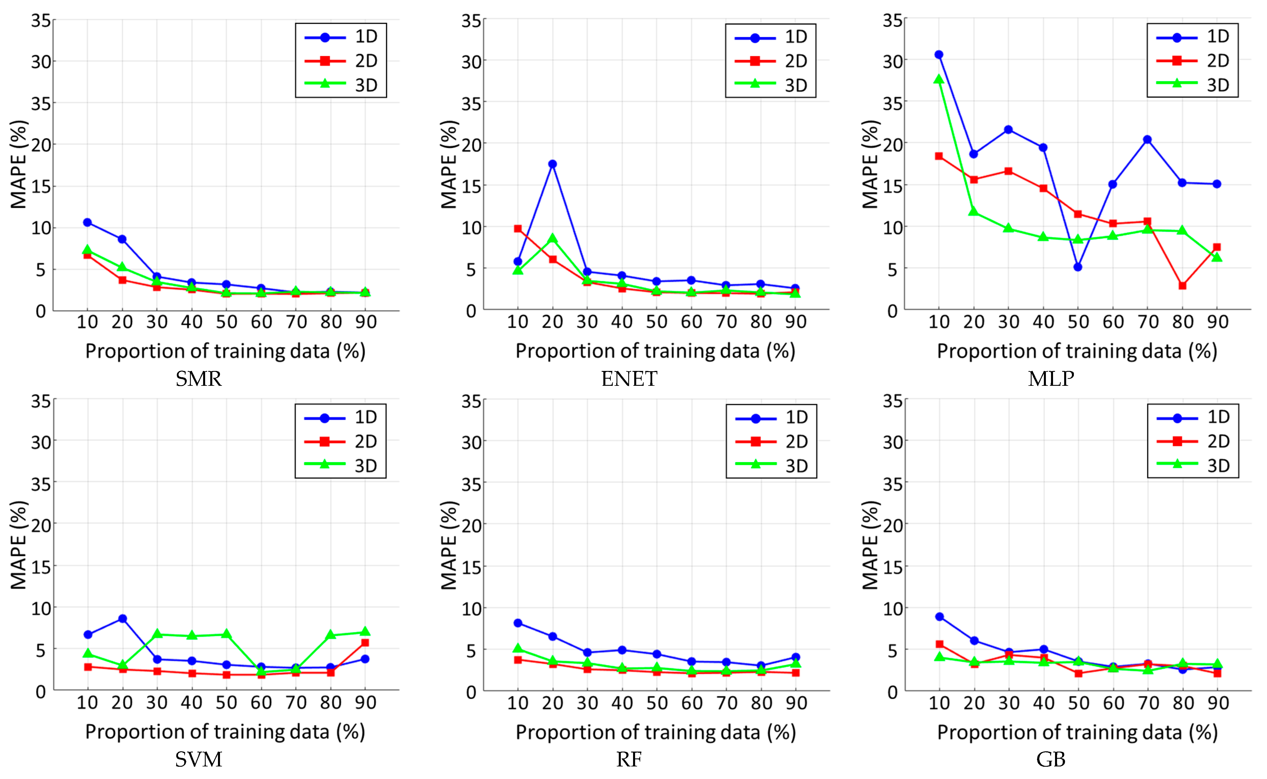
Figure 4 shows charts of MAPE for each movement type and the proportion of training data, categorized by six model types. In most cases, a higher proportion of training data tends to lead to improved prediction performance. However, in certain cases (e.g., 1D movement of SVM, RF, and GB, 2D movement of ENET, MLP, and SVM, and 3D movement of SVM and RF), MAPE increases when the proportion of training data reaches 90%. This phenomenon provides the insight that an increase in the amount of training data does not necessarily lead to improved prediction performance. Moreover, the variation in MAPE by various proportions of training data can serve as a basis for optimizing the cost and effort of data collection in practical applications. In addition, six model types show a common trend; MAPE for 1D movement is typically higher than those for 2D and 3D movements.

To statistically validate these findings and understand their underlying causes, we perform an ANOVA and a GLM analysis. The ANOVA results, summarized in

Table 11. ANOVA table.

Source	Sum of Squares	Degree of Freedom	Mean Square	F	p-Value	${\mathit{\eta }}^2$
Corrected model	2931.91	15	195.461	27.406	0.000	0.738
Intercept	4712.907	1	4712.907	660.796	0.000	0.819
Proportion of training data	547.565	8	68.446	9.597	0.000	0.345
Movement type	168.153	2	84.076	11.788	0.000	0.139
Model type	2216.192	5	443.238	62.146	0.000	0.680
Error	1041.296	146	7.132
Total	8686.113	162
Corrected Total	3973.206	161

, confirm that the model type, movement type, and proportion of training data all have a statistically significant effect on MAPE (p-value = 0.000).

In addition, the GLM estimation results provide a more detailed confirmation of our initial observations (

Table 12. GLM estimation results.

Factor	Level	Coefficient	Robust Standard Error	t	p-Value
Intercept		2.229	0.839	2.656	0.009
Movement type	1D	1.959	0.514	3.812	0.000
	2D	−0.359	0.514	−0.698	0.486
	3D	0
Model type	ENET	0.119	0.727	0.164	0.870
	GB	−0.249	0.727	−0.342	0.733
	MLP	9.716	0.727	13.368	0.000
	RF	−0.460	0.727	−0.632	0.528
	SMR	−0.378	0.727	−0.521	0.603
	SVM	0
Proportion of training data	10%	5.253	0.890	5.901	0.000
	20%	3.315	0.890	3.724	0.000
	30%	1.644	0.890	1.847	0.067
	40%	1.099	0.890	1.234	0.219
	50%	−0.313	0.890	−0.352	0.725
	60%	−0.224	0.890	−0.251	0.802
	70%	0.146	0.890	0.164	0.870
	80%	−0.365	0.890	−0.410	0.682
	90%	0

). For model types, there is no statistically significant difference in performance between SVM and all other model types, except for MLP. The large, positive, and highly significant coefficient for MLP (coefficient = 9.716 and p-value = 0.000) indicates poorer performance compared to other model types. In other words, relative to SVM, MLP increases expected MAPE by about 9.716 percentage points. Similarly, 1D movement is significantly more challenging to predict (coefficient = 1.959, p-value = 0.000), increasing expected MAPE (i.e., prediction error) by about 1.959 percentage points relative to the 3D movement. Conversely, there is no significant performance difference between 2D and 3D movements (p-value = 0.486). Moreover, for the proportion of training data, the GLM analysis reveals that using small datasets (10% to 30%) significantly increases prediction error. However, the other levels (40% to 80%) show no statistically significant difference in MAPE compared to 90%.

To investigate why the power of 1D movement is more difficult to predict, we compare the variance of the power demand data across movement types using the F-test (

Table 13. Comparison of power demand data across movement types (F-test results).

	Group 1		Group 2		Group 3
	1D	2D	1D	3D	2D	3D
Mean (power demand [W])	65.124	65.035	65.124	65.425	65.035	65.425
Variance (power demand [W])	33.385	22.261	33.385	22.450	22.261	22.450
Number of observations	510	1000	510	590	1000	590
F-value	1.500		1.487		0.992
p-value	0.000		0.000		0.452

). The test reveals that the data from 1D movements has significantly larger variance than that from 2D and 3D movements (p-value = 0.000).

The findings from MAPE comparison and GLM provide a foundational, high-level performance evaluation across all experimental factors, yielding three key insights. First, while the MLP shows the poorest performance at a statistically significant level, the other five model types are not distinguishable based on predictive accuracy alone. This finding underscores that accuracy alone is an insufficient metric for power prediction model selection, necessitating the multi-criteria evaluation. Second, the analyses identify a distinct performance pattern among the movement types. One-dimensional movements yield higher prediction errors compared to both 2D and 3D movements. This finding is explained by the data’s inherent statistical properties, as our analysis shows that the power data from 1D movements exhibit significantly higher variance. Finally, in our dataset, a minimum of 40% training data is sufficient to prevent a significant accuracy drop. However, this finding is limited to our experimental data and should be considered an example. Taken together, the results show that accuracy alone is not a sufficient criterion to choose an RA power prediction model. Thus, in the following subsections, we compare RA power prediction models by incorporating one additional criterion: training time. More specifically, we select the best model that is both accurate and fast to train. Then, we explain the physical reasons behind the power prediction model’s performance. Especially to provide more actionable and context-specific guidance for shop-floor engineers, our subsequent analyses are conducted for each movement type separately.

4.2. Pareto Frontier: Trade-Off Analysis of MAPE vs. Training Time

Alongside the prediction performance of the models, the time required for training is also an important aspect for selecting an appropriate model. Thus, we utilize the Pareto frontier to visualize the trade-off relationship between the performance and training time of RA power prediction models. Specifically, the Pareto frontier is constructed individually for each movement type. Additionally, since the data points are concentrated near zero and therefore difficult to distinguish, we apply a logarithmic scale to the X-axis of the Pareto frontier (training time). Figure 5a–c display MAPE versus training time for all 54 RA power prediction models for 1D, 2D, and 3D movement, respectively. Each prediction model is displayed with a different marker according to model type, and the Pareto frontier is drawn as a black, solid line.

For 1D movement, the model types of the prediction models on the Pareto frontier are SVM and SMR. In the case of 2D movement, SVM is the only model type found on the Pareto frontier. For 3D movement, the model types on the Pareto frontier are SVM, SMR, and ENET. Overall, power prediction models developed based on the SVM model type consistently appear on the Pareto frontier for all three movement types.

Table 14. Movement type, model type, and training data proportion for the Pareto frontier.

Movement Type	Model Type	Proportion of Training Data	MAPE	Training Time (Seconds)
1D	SMR	90%	2.222	6.696
	SMR	70%	2.251	5.654
	SMR	80%	2.334	5.228
	SVM	70%	2.694	3.031
	SVM	80%	2.746	1.430
	SVM	60%	2.813	0.384
	SVM	40%	3.53	0.248
	SVM	30%	3.707	0.055
2D	SVM	60%	1.862	4.925
	SVM	50%	1.867	3.023
	SVM	40%	2.042	2.303
	SVM	70%	2.31	0.370
	SVM	20%	2.492	0.083
	SVM	10%	2.828	0.053
3D	ENET	90%	1.856	21.261
	ENET	60%	2.045	16.183
	SMR	60%	2.132	4.388
	SMR	50%	2.157	4.375
	SVM	60%	2.177	1.285
	SVM	20%	2.972	0.052

presents the comparison factors (movement type, model type, and proportion of training data) corresponding to each point on the Pareto frontier.

Among models on three Pareto frontiers, SVM with a proportion of training data at 60% appears across all three movements. This result indicates that for our specific dataset, using about 60% of the data is sufficient to achieve both low prediction error and short training time. Increasing the training data beyond 60% does not necessarily improve accuracy, while it substantially increases training time. The required minimum number of training data also reflects the absolute number of observations. For 1D and 3D movements, the total sample sizes are smaller than 2D (510 and 590, respectively), and so prediction models with up to 90% training data appear on the Pareto frontier. In contrast, 2D has the largest sample size (1000), and the Pareto frontier includes models with at most 70% training data. This suggests that the trade-off between the power prediction model’s performance and training time is highly influenced by the amount of training data.

All of the most inefficient models (i.e., models located in the upper-right region of the plots in Figure 5) are based on MLP. That is, models of the MLP type show long training times and low predictive accuracy. In particular, MLP models with training data proportions of 10%, 30%, and 70% consistently fall on solutions dominated by the Pareto frontiers across all three movements. These results highlight that in data-driven regression model building, the balance among training data size, predictive accuracy, and computational cost must be carefully considered.

4.3. SHAP: XAI for Physical Features and Power Prediction

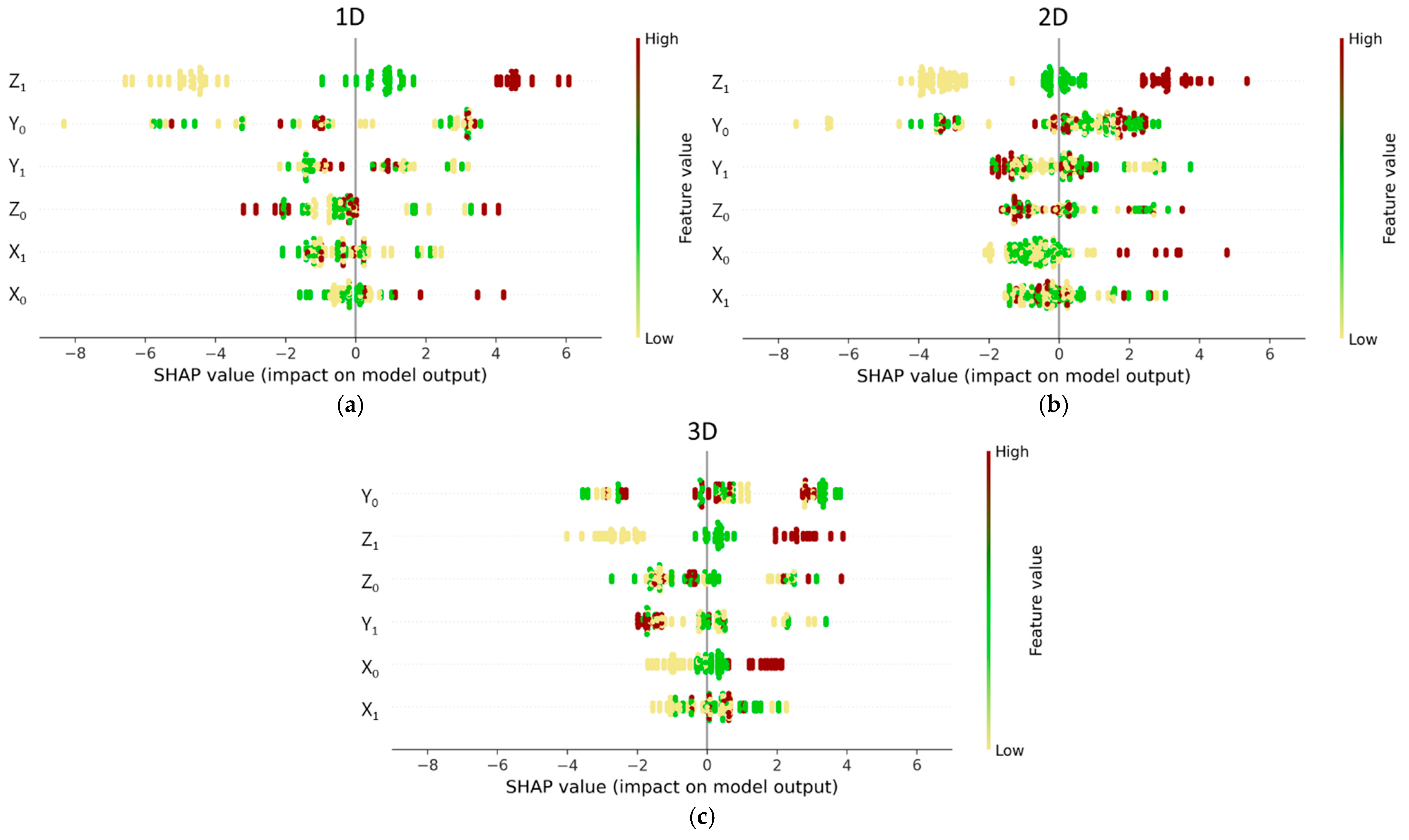
To further investigate the results of the Pareto frontier analysis, we conduct SHAP analysis for two models: SVM (training data 60%) and MLP (training data 10%). The SVM with training data at 60% appears on the Pareto frontier across all three movements, consistently demonstrating good predictive performance with short training time. In contrast, the MLP with training data 10% shows the highest MAPE among the inefficient models, consistently across all three movements. These two contrasting models are therefore selected for SHAP analysis as best-performing and worst-performing models, respectively. Figure 6 presents the SHAP plots of the SVM model (training data 60%) for power prediction of 1D, 2D, and 3D movements.

For the 1D movement power prediction (Figure 6a), Z₁ (Z-coordinate of the ending point) is identified as the most influential feature. In the SHAP plot of 2D movement (Figure 6b), Z₁ emerges again as the most important feature. For 3D movements, unlike in 1D and 2D, Y₀ (Y-coordinate of the starting point) is the most influential feature, followed by Z₁ as the second-most influential feature (Figure 6c).

According to the physical characteristics of RA movements, when the end effector moves upward (against gravity), joint torque increases and significantly affects power consumption [14,71,72]. In other words, due to the effect of gravity, Z₁ inevitably exerts a meaningful influence on power demand. The SVM model (training data 60%) effectively captures this embedded information in the data, making appropriate use of the features for prediction. For these reasons, Z₁ is identified as the most important feature for 1D and 2D movements and the second-most important for 3D movement. Moreover, the SHAP plots for all three movements in Figure 6 show a highly linear relationship between the Z₁ feature value and its corresponding SHAP value with clear separation of colors. Specifically, the increase in Z₁ value increases the predicted power value.

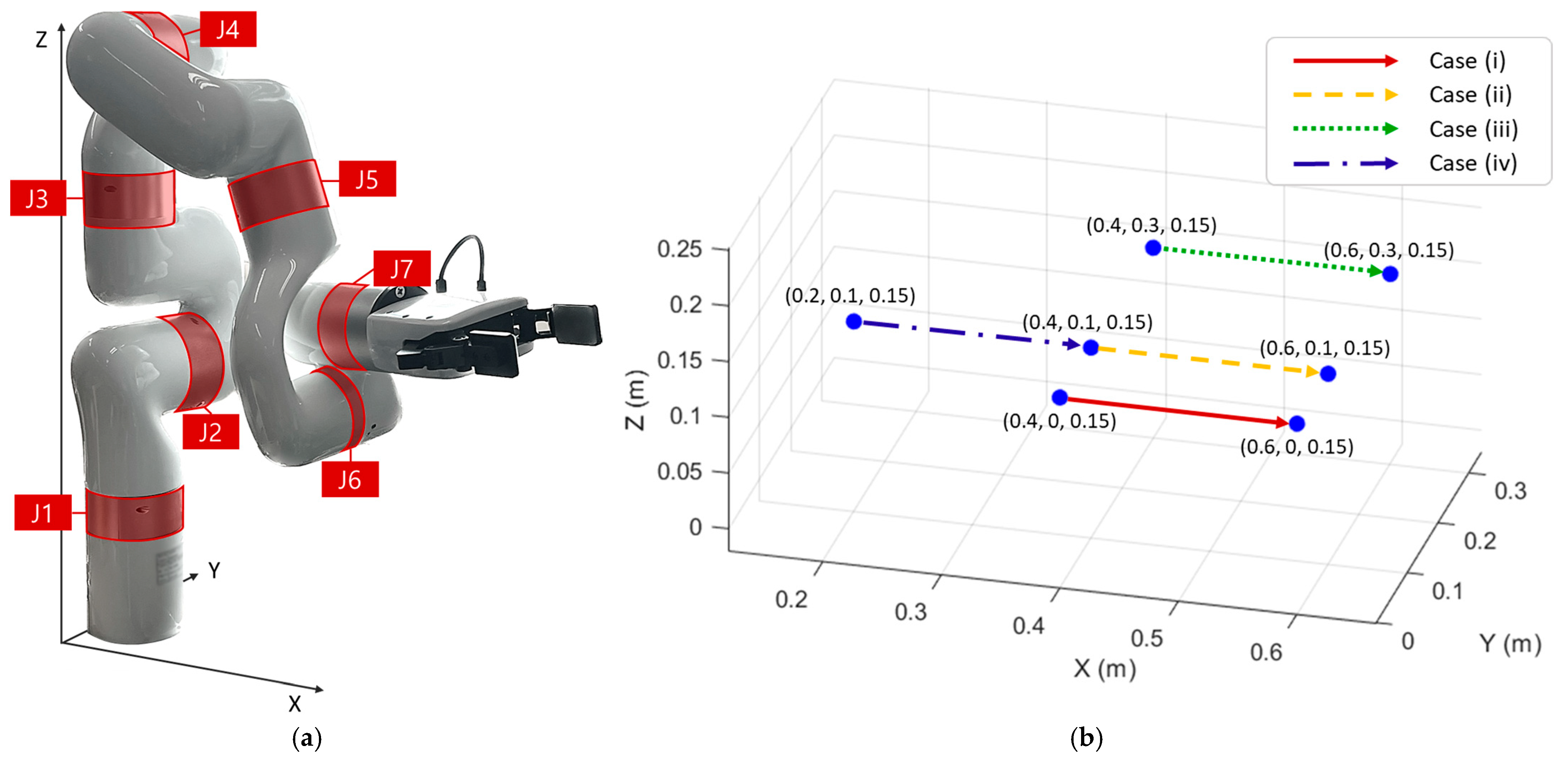
In addition, for all movement types, Y₀ and Y₁ (Y-coordinate of the starting and ending points) exhibit higher importance compared to X₀ and X₁ (X-coordinate of the starting and ending points). This aligns with the physical observation that lateral displacement (Y-axis) induces larger variations in joint trajectories than forward-backward displacement along the X-axis. To examine the influence of X- and Y-coordinates on seven joints (J1 to J7 as in Figure 7a) of the RA, we present experimental observations across four movement cases as shown in Figure 7b. These cases are selected from the coordinate set used in the power data collection experiment (Figure 2), so that they represent specific examples within our experimental design.

Table 15. Joint angles at the start and end of Cases (i)–(iv) and their differences.

	Case (i)			Case (ii)			Case (iii)			Case (iv)
Joint	Joint Angle (°)
	Start	End	Difference	Start	End	Difference	Start	End	Difference	Start	End	Difference
J1	0	0	0	12.9	8	4.9	30	24.4	5.6	18.6	12.9	5.7
J2	14.8	42.3	27.5	16.4	43.8	27.4	27.9	56.2	28.3	−10.6	16.4	27
J3	0	0	0	1	1.8	0.8	6.7	3.4	3.3	11.6	1	10.6
J4	36.5	84.6	48.1	39	87.2	48.2	58.4	110	51.6	2	39	37
J5	0	0	0	−0.8	−1.8	1	−6.1	−3.5	2.6	9.7	−0.8	10.5
J6	21.6	42.3	20.7	22.6	43.5	20.9	30.8	53.9	23.1	12.6	22.6	10
J7	0	0	0	14.6	10.6	4	41.2	28.3	12.9	20.5	14.6	5.9
Average			13.76			15.31			18.20			15.24

presents the joint angles at the start and end of four movement cases, along with their differences. The comparison of Cases (i), (ii), and (iii) shows that larger Y-coordinate values lead to greater changes in the joint angles. Specifically, the average differences across the seven joints are 13.76, 15.31, and 18.20, respectively. In particular, for J1, J3, J5, and J7, no movement occurs when the Y-coordinate is zero under single-axis motion along the X-direction (Case (i)). In contrast, the comparison of Cases (ii) and (iv) shows that the increase in the X-coordinate does not result in significant differences in joint movement (15.24 and 15.31). These observations indicate that, for the RA employed in this experiment, the Y-coordinate (i.e., lateral displacement from the center) has a stronger influence on joint angle change than the X-coordinate (i.e., forward-backward displacement). Additionally, the SVM model (training data 60%) effectively captures this property from the data, as reflected by the higher importance of Y₀ and Y₁ compared to X₀ and X₁. Moreover, analysis of the color of the SHAP plots in Figure 6 reveals that, unlike Z₁, the relationships between the feature value of Y₀, Y₁, and their SHAP values are not strictly linear. In other words, in power prediction, the Y-coordinates have substantial interaction effects with other features.

Taken together, the importance of the features utilized by SVM (training data 60%) for power prediction is consistently aligned with physical principles: (i) Z₁ is important because it reflects gravitational effects across all movement types, (ii) Y-coordinates have strong influence compared to X-coordinates, reflecting the structural dynamics of the RA, and (iii) interaction effects become more pronounced in higher-dimensional movements. These results explain why SVM (training data 60%) consistently appeared on the Pareto frontiers of all movement types.

The MLP model (training data 10%) shows markedly different SHAP patterns. As shown in Figure 8, Z₀ and Z₁ relatively show low importance across 1D, 2D, and 3D movements, indicating that the model failed to capture the effect of gravity, a fundamental driver of power consumption. Instead, the model assigns abnormally high importance to features such as X₀ and X₁, with absolute SHAP values far exceeding those observed in SVM (training data 60%). This suggests that MLP (training data 10%) overfits to local data patterns, relying excessively on less relevant features and neglecting physically meaningful ones. In other words, MLP fails to capture the critical patterns among features and does not effectively exploit the embedded information in the data. Thus, MLP (training data 10%) shows consistently poor predictive performance and high MAPE, compared with SVM (training data 60%).

Our analysis provides explainable guidance for shop-floor RA energy management. SHAP results indicate that high-performing models, such as SVM, succeed because they not only fit the data but also learn the RA’s physical characteristics embedded in the power data. SVM consistently assigns high importance to Z-axis motion, reflecting gravitational load. SVM also separates the asymmetric effects of lateral (Y-axis) and forward (X-axis) motion: the distinct joint-angle trajectories generate different torque requirements, leading to different power demands. In contrast, MLP does not capture these relationships between physical patterns and the power demand of RA’s movement, resulting in poor accuracy. These findings show that capturing the relevant physics in the data directly drives predictive performance.

The results of our analysis provide critical insights that are not limited to a simple accuracy comparison, directly addressing the need for explainable and practical RA energy management tools on the shop floor. Particularly, the SHAP analysis reveals that the excellence of the well-performing model is not just about predictive accuracy. The accurate power prediction model can successfully learn the underlying physical principles of the RA operation. For instance, SVM (training data 60%) consistently recognizes the importance of Z-axis movement due to gravity. Moreover, SVM (training data 60%) captures the asymmetrical impact of lateral (Y-axis) versus forward (X-axis) movements. As our joint angle analysis shows, these seemingly similar horizontal movements (along X and Y axes) result in vastly different kinematic changes and different power demands of RA. In contrast, the MLP (training data 10%) fails to capture the fundamental physical features and therefore shows poor predictive performance. These results highlight that the RA power prediction model’s ability to capture the physics embedded in the data is an important driver of its predictive success.

The results also highlight the core contribution of our study: energy consumption of RA is highly connected to operational factors in ways that are often counterintuitive. In terms of energy consumption, moving a certain distance along the X-axis might intuitively be considered equivalent to moving the same distance along the Y-axis by a shop-floor engineer. However, our findings show that this intuition is not true. The energy consumption of an RA is deeply dependent on the specific trajectory and how that trajectory determines the RA’s joints to act against physical forces such as gravity and inertia. Therefore, relying on intuition alone for RA energy management is inadequate, and it is important to adopt data-driven, analytical approaches, as we presented. These insights have significant implications for RA task design in manufacturing. For any given task, defined by a starting and ending point, there exists a near-infinite number of feasible trajectories. Thus, finding the energy-efficient path among all possible routes can offer significant potential for energy saving. For example, a simple straight-line path might not be the most energy-efficient if it involves significant lateral movement that strains specific joints. In such cases, a slightly curved path can reduce the high-load movements and result in the same production outcome with substantial energy savings. With the insights offered by our analysis, shop-floor engineers can critically assess the software-generated RA trajectories and select energy-efficient trajectories for performing the required task. The framework and RA power prediction models validated in this study provide the foundational tools necessary to find such energy-efficient RA paths.

Consequently, our findings in this study provide several key contributions for RA energy management. First, the results suggest that an SVM model, trained with an appropriate amount of data, can be a robust recommendation. Furthermore, shop-floor engineers operating RA can readily develop and utilize power prediction models by referring to the detailed information provided in this study, such as hyperparameter settings. Moreover, the XAI analysis reveals a counterintuitive insight: seemingly similar horizontal movements (along X and Y axes) can have different power demands. These findings underscore that relying on intuition is insufficient and that careful, model-driven examination is essential to design RA tasks for energy efficiency.

5. Conclusions

This study aims to identify a ready-to-use RA power prediction model that helps shop-floor engineers understand and manage RA energy consumption. To find such a model, we introduce a novel comparison framework that considers not only the accuracy of the power prediction model but also RA’s movement and proportion of training data. For developing the proposed framework, we first set three experimental factors (i.e., model type, movement type, and proportion of training data) and their levels for comparing power prediction models. We then collect a total of 2100 power data of 1D, 2D, and 3D movements of a 7-DOF RA, and for each experimental factor, power prediction models are developed and trained. Next, we conduct a comprehensive statistical analysis of predictive accuracy, using GLM to validate the influence of three factors. Additionally, the Pareto frontier is utilized to identify the most practically useful models by incorporating training time. Lastly, SHAP analysis is conducted on the best and worst-performing models identified from the Pareto analysis to explain how their predictions link to the RA’s physical dynamics.

The analysis results show that most model types (except for the underperforming MLP) have statistically similar accuracy. The GLM and F-test analyses show that the cause of high prediction error is the high variance of the power data. The Pareto frontier highlights SVM as a highly efficient choice, balancing low prediction error with short training times across all movement types. SHAP analysis confirmed the reason for this superiority: the SVM model (training data 60%) effectively captures the physical drivers of power consumption. In contrast, the MLP model (training data 10%) fails to recognize even fundamental physical principles, such as gravity, so it shows the worst prediction performance.

The primary contribution of this research is the establishment of a multi-criteria comparison framework that bridges the gap between theoretical power prediction modeling and actual shop-floor energy management. This framework offers practitioners context-based guidelines on RA power prediction model selection based on specific operational contexts and the amount of available data. Moreover, we propose detailed guidance on how to develop the RA power prediction models (including hyperparameter tuning). In addition, our work also delivers actionable insights into how an RA’s trajectory influences power demand, enabling shop-floor engineers to design more energy-efficient tasks. Furthermore, this study highlights the essential role of XAI within the proposed framework. In particular, SHAP is used not merely for explanation but as a core evaluation tool that reveals whether each prediction model captures the physical dynamics underlying RA power demands. XAI analysis enhances interpretability by explaining the behavior of black-box AI models through their relationships with input features. Thus, XAI can help shop-floor engineers who may not be familiar with AI understand the prediction models’ results and behavior.

Nevertheless, the scope of this study is limited to specific equipment and experimental conditions, which may constrain the generalizability of the results. Future studies will extend the framework by considering different robot models or physical parameters to evaluate the generalizability of the proposed approach under diverse operational settings. In addition, future studies will systemically investigate the performance differences across model types by analyzing their internal learning mechanisms.

References

1. Appleton, E.; Williams, D.J. Industrial Robot Applications; Springer Science & Business Media: Dordrecht, The Netherlands, 2012; ISBN 978-94-009-3125-1. [Google Scholar]
2. Li, X.; Yang, X.; Zhao, Y.; Teng, Y.; Dong, Y. Metaheuristic for Solving Multi-Objective Job Shop Scheduling Problem in a Robotic Cell. IEEE Access 2020, 8, 147015–147028. [Google Scholar] [CrossRef]
3. Foumani, M.; Gunawan, I.; Smith-Miles, K.; Ibrahim, M.Y. Notes on Feasibility and Optimality Conditions of Small-Scale Multifunction Robotic Cell Scheduling Problems with Pickup Restrictions. IEEE Trans. Ind. Inform. 2015, 11, 821–829. [Google Scholar] [CrossRef]
4. Industrial Robots Market Size, Share, Industry Growth, 2032. Available online: https://www.fortunebusinessinsights.com/industry-reports/industrial-robots-market-100360 (accessed on 18 August 2025).
5. International Federation of Robotics (Ed.) World Robotics 2022: Industrial Robots; VDMA Services GmbH: Franckfurt, Germany, 2022; ISBN 978-3-8163-0752-5. [Google Scholar]
6. Garriz, C.; Domingo, R. Trajectory Optimization in Terms of Energy and Performance of an Industrial Robot in the Manufacturing Industry. Sensors 2022, 22, 7538. [Google Scholar] [CrossRef]
7. Huang, G.; He, L.-Y.; Lin, X. Robot Adoption and Energy Performance: Evidence from Chinese Industrial Firms. Energy Econ. 2022, 107, 105837. [Google Scholar] [CrossRef]
8. Pedersen, M.R.; Nalpantidis, L.; Andersen, R.S.; Schou, C.; Bøgh, S.; Krüger, V.; Madsen, O. Robot Skills for Manufacturing: From Concept to Industrial Deployment. Robot. Comput. Integr. Manuf. 2016, 37, 282–291. [Google Scholar] [CrossRef]
9. Li, Y.; Badulescu, A.; Badulescu, D. Modeling and Analyzing Critical Policies for Improving Energy Efficiency in Manufacturing Sector: An Interpretive Structural Modeling (ISM) Approach. Energies 2025, 18, 893. [Google Scholar] [CrossRef]
10. Gadaleta, M.; Pellicciari, M.; Berselli, G. Optimization of the Energy Consumption of Industrial Robots for Automatic Code Generation. Robot. Comput. Integr. Manuf. 2019, 57, 452–464. [Google Scholar] [CrossRef]
11. Soori, M.; Arezoo, B.; Dastres, R. Optimization of Energy Consumption in Industrial Robots, a Review. Cogn. Robot. 2023, 3, 142–157. [Google Scholar] [CrossRef]
12. Walther, J.; Weigold, M. A Systematic Review on Predicting and Forecasting the Electrical Energy Consumption in the Manufacturing Industry. Energies 2021, 14, 968. [Google Scholar] [CrossRef]
13. Kebria, P.M.; Al-wais, S.; Abdi, H.; Nahavandi, S. Kinematic and Dynamic Modelling of UR5 Manipulator. In Proceedings of the 2016 IEEE International Conference on Systems, Man, and Cybernetics (SMC), Budapest, Hungary, 9–12 October 2016; pp. 004229–004234. [Google Scholar]
14. Jung, S.Y.; Jeon, H.W.; Park, K. Power Estimation Models of a 7-Axis Robotic Arm with Simulated Manufacturing Applications. Int. J. Adv. Manuf. Technol. 2024, 134, 4161–4185. [Google Scholar] [CrossRef]
15. Chen, Z.; Xiao, F.; Guo, F.; Yan, J. Interpretable Machine Learning for Building Energy Management: A State-of-the-Art Review. Adv. Appl. Energy 2023, 9, 100123. [Google Scholar] [CrossRef]
16. Chen, T.-C.T. Explainable Artificial Intelligence (XAI) in Manufacturing. In Explainable Artificial Intelligence (XAI) in Manufacturing: Methodology, Tools, and Applications; Chen, T.-C.T., Ed.; Springer International Publishing: Cham, Switzerland, 2023; pp. 1–11. ISBN 978-3-031-27961-4. [Google Scholar]
17. Yin, S.; Ji, W.; Wang, L. A Machine Learning Based Energy Efficient Trajectory Planning Approach for Industrial Robots. Procedia CIRP 2019, 81, 429–434. [Google Scholar] [CrossRef]
18. Wallén, J. The History of the Industrial Robot; Linköping University Electronic Press: Linköping, Sweden, 2008. [Google Scholar]
19. Arents, J.; Greitans, M. Smart Industrial Robot Control Trends, Challenges and Opportunities within Manufacturing. Appl. Sci. 2022, 12, 937. [Google Scholar] [CrossRef]
20. Vyas, V.; Jeon, H.W. Estimating Energy Costs by Simulating Dependence between Turning Parameters. In Proceedings of the 2020 IISE Annual Conference, Virtual, 1–3 November 2020; pp. 340–345. [Google Scholar]
21. Mahdavian, M.; Shariat-Panahi, M.; Yousefi-Koma, A.; Ghasemi-Toudeshki, A. Optimal Trajectory Generation for Energy Consumption Minimization and Moving Obstacle Avoidance of a 4DOF Robot Arm. In Proceedings of the 2015 3rd RSI International Conference on Robotics and Mechatronics (ICROM), Tehran, Iran, 7–9 October 2015; pp. 353–358. [Google Scholar]
22. Mohammed, A.; Schmidt, B.; Wang, L.; Gao, L. Minimizing Energy Consumption for Robot Arm Movement. Procedia CIRP 2014, 25, 400–405. [Google Scholar] [CrossRef]
23. Chemnitz, M.; Schreck, G.; Kruger, J. Analyzing Energy Consumption of Industrial Robots. In Proceedings of the ETFA2011, Toulouse, France, 5–9 September 2011; pp. 1–4. [Google Scholar]
24. Garcia, R.R.; Bittencourt, A.C.; Villani, E. Relevant Factors for the Energy Consumption of Industrial Robots. J. Braz. Soc. Mech. Sci. Eng. 2018, 40, 464. [Google Scholar] [CrossRef]
25. Guerra-Zubiaga, D.A.; Luong, K.Y. Energy Consumption Parameter Analysis of Industrial Robots Using Design of Experiment Methodology. Int. J. Sustain. Eng. 2021, 14, 996–1005. [Google Scholar] [CrossRef]
26. Lin, H.-I.; Mandal, R.; Wibowo, F.S. BN-LSTM-Based Energy Consumption Modeling Approach for an Industrial Robot Manipulator. Robot. Comput. Integr. Manuf. 2024, 85, 102629. [Google Scholar] [CrossRef]
27. Yan, J.; Zhang, M. A Transfer-Learning Based Energy Consumption Modeling Method for Industrial Robots. J. Clean. Prod. 2021, 325, 129299. [Google Scholar] [CrossRef]
28. Yao, M.; Zhao, Q.; Shao, Z.; Zhao, Y. Research on Power Modeling of the Industrial Robot Based on ResNet. In Proceedings of the 2022 7th International Conference on Automation, Control and Robotics Engineering (CACRE), Xi’an, China, 14–16 July 2022; pp. 87–92. [Google Scholar]
29. Forkuor, G.; Hounkpatin, O.K.L.; Welp, G.; Thiel, M. High Resolution Mapping of Soil Properties Using Remote Sensing Variables in South-Western Burkina Faso: A Comparison of Machine Learning and Multiple Linear Regression Models. PLoS ONE 2017, 12, e0170478. [Google Scholar] [CrossRef]
30. Wu, C.-S.M.; Patil, P.; Gunaseelan, S. Comparison of Different Machine Learning Algorithms for Multiple Regression on Black Friday Sales Data. In Proceedings of the 2018 IEEE 9th International Conference on Software Engineering and Service Science (ICSESS), Beijing, China, 23–25 January 2018; pp. 16–20. [Google Scholar]
31. Acharya, M.S.; Armaan, A.; Antony, A.S. A Comparison of Regression Models for Prediction of Graduate Admissions. In Proceedings of the 2019 International Conference on Computational Intelligence in Data Science (ICCIDS), Chennai, India, 21–23 February 2019; pp. 1–5. [Google Scholar]
32. Park, J.-W.; Kang, B.-S. Comparison between Regression and Artificial Neural Network for Prediction Model of Flexibly Reconfigurable Roll Forming Process. Int. J. Adv. Manuf. Technol. 2019, 101, 3081–3091. [Google Scholar] [CrossRef]
33. Leng, G.; Hall, J.W. Predicting Spatial and Temporal Variability in Crop Yields: An Inter-Comparison of Machine Learning, Regression and Process-Based Models. Environ. Res. Lett. 2020, 15, 044027. [Google Scholar] [CrossRef] [PubMed]
34. Kim, Y.; Oh, H. Comparison between Multiple Regression Analysis, Polynomial Regression Analysis, and an Artificial Neural Network for Tensile Strength Prediction of BFRP and GFRP. Materials 2021, 14, 4861. [Google Scholar] [CrossRef] [PubMed]
35. Dabiri, H.; Rahimzadeh, K.; Kheyroddin, A. A Comparison of Machine Learning- and Regression-Based Models for Predicting Ductility Ratio of RC Beam-Column Joints. Structures 2022, 37, 69–81. [Google Scholar] [CrossRef]
36. Mohammed, S.; Jouhra, A.; Enaruvbe, G.O.; Bashir, B.; Barakat, M.; Alsilibe, F.; Cimusa Kulimushi, L.; Alsalman, A.; Szabó, S. Performance Evaluation of Machine Learning Algorithms to Assess Soil Erosion in Mediterranean Farmland: A Case-Study in Syria. Land Degrad. Dev. 2023, 34, 2896–2911. [Google Scholar] [CrossRef]
37. Satpathi, A.; Setiya, P.; Das, B.; Nain, A.S.; Jha, P.K.; Singh, S.; Singh, S. Comparative Analysis of Statistical and Machine Learning Techniques for Rice Yield Forecasting for Chhattisgarh, India. Sustainability 2023, 15, 2786. [Google Scholar] [CrossRef]
38. Archontoulis, S.V.; Miguez, F.E. Nonlinear Regression Models and Applications in Agricultural Research. Agron. J. 2015, 107, 786–798. [Google Scholar] [CrossRef]
39. Kutner, M.H.; Nachtsheim, C.J.; Neter, J. Applied Linear Regression Models; McGraw Hill: New York, NY, USA, 2008. [Google Scholar]
40. Lotov, A.V.; Miettinen, K. Visualizing the Pareto Frontier. In Multiobjective Optimization: Interactive and Evolutionary Approaches; Branke, J., Deb, K., Miettinen, K., Słowiński, R., Eds.; Springer: Berlin/Heidelberg, Germany, 2008; pp. 213–243. ISBN 978-3-540-88908-3. [Google Scholar]
41. Lackner, K.S.; Wendt, C.H.; Butt, D.P.; Joyce, E.L.; Sharp, D.H. Carbon Dioxide Disposal in Carbonate Minerals. Energy 1995, 20, 1153–1170. [Google Scholar] [CrossRef]
42. Nohara, Y.; Matsumoto, K.; Soejima, H.; Nakashima, N. Explanation of Machine Learning Models Using Shapley Additive Explanation and Application for Real Data in Hospital. Comput. Methods Programs Biomed. 2022, 214, 106584. [Google Scholar] [CrossRef]
43. Li, Z. Extracting Spatial Effects from Machine Learning Model Using Local Interpretation Method: An Example of SHAP and XGBoost. Comput. Environ. Urban Syst. 2022, 96, 101845. [Google Scholar] [CrossRef]
44. X-ARM|UFACTORY. Available online: https://www.ufactory.us/xarm (accessed on 19 August 2025).
45. Fluke 1732 and 1734 Three Phase Power Measurement Logger|Fluke. Available online: https://www.fluke.com/en-us/product/electrical-testing/power-quality/1732-1734 (accessed on 19 August 2025).
46. Spiliotis, E.; Makridakis, S.; Semenoglou, A.-A.; Assimakopoulos, V. Comparison of Statistical and Machine Learning Methods for Daily SKU Demand Forecasting. Oper. Res. 2022, 22, 3037–3061. [Google Scholar] [CrossRef]
47. Hu, Y.; Sun, Z.; Pei, L.; Li, W.; Li, Y. Evaluation of Pavement Surface Roughness Performance under Multi-Features Conditions Based on Optimized Random Forest. In Proceedings of the 2021 Ninth International Conference on Advanced Cloud and Big Data (CBD), Xi’an, China, 26–27 March 2022; pp. 133–138. [Google Scholar]
48. Noryani, M.; Sapuan, S.M.; Mastura, M.T.; Zuhri, M.Y.M.; Zainudin, E.S. Material Selection of Natural Fibre Using a Stepwise Regression Model with Error Analysis. J. Mater. Res. Technol. 2019, 8, 2865–2879. [Google Scholar] [CrossRef]
49. Tibshirani, R. Regression Shrinkage and Selection Via the Lasso. J. R. Stat. Soc. Ser. B-Stat. Methodol. 1996, 58, 267–288. [Google Scholar] [CrossRef]
50. Aldahmani, S.; Zoubeidi, T. Graphical Group Ridge. J. Stat. Comput. Simul. 2020, 90, 3422–3432. [Google Scholar] [CrossRef]
51. Zou, H.; Hastie, T. Regularization and Variable Selection Via the Elastic Net. J. R. Stat. Soc. Ser. B Stat. Methodol. 2005, 67, 301–320. [Google Scholar] [CrossRef]
52. Huang, Y. Advances in Artificial Neural Networks—Methodological Development and Application. Algorithms 2009, 2, 973–1007. [Google Scholar] [CrossRef]
53. Yu, D.; Deng, L. Efficient and Effective Algorithms for Training Single-Hidden-Layer Neural Networks. Pattern Recognit. Lett. 2012, 33, 554–558. [Google Scholar] [CrossRef]
54. Doukim, C.A.; Dargham, J.A.; Chekima, A. Finding the Number of Hidden Neurons for an MLP Neural Network Using Coarse to Fine Search Technique. In Proceedings of the 10th International Conference on Information Science, Signal Processing and their Applications (ISSPA 2010), Kuala Lumpur, Malaysia, 10–13 May 2010; pp. 606–609. [Google Scholar]
55. Samatin Njikam, A.N.; Zhao, H. A Novel Activation Function for Multilayer Feed-Forward Neural Networks. Appl. Intell. 2016, 45, 75–82. [Google Scholar] [CrossRef]
56. Wilson, D.R.; Martinez, T.R. The Need for Small Learning Rates on Large Problems. In Proceedings of the IJCNN’01, International Joint Conference on Neural Networks, Proceedings (Cat. No.01CH37222), Washington, DC, USA, 15–19 July 2001; Volume 1, pp. 115–119. [Google Scholar]
57. Gao, J.B.; Gunn, S.R.; Harris, C.J.; Brown, M. A Probabilistic Framework for SVM Regression and Error Bar Estimation. Mach. Learn. 2002, 46, 71–89. [Google Scholar] [CrossRef]
58. Jakkula, V. Tutorial on Support Vector Machine (SVM). Sch. EECS Wash. State Univ. 2006, 37, 3. [Google Scholar]
59. Hsu, C.-W.; Chang, C.-C.; Lin, C.-J. A Practical Guide to Support Vector Classification. 2003, pp. 1396–1400. Available online: https://www.csie.ntu.edu.tw/~cjlin/papers/guide/guide.pdf (accessed on 19 August 2025).
60. Hussain, M.; Wajid, S.K.; Elzaart, A.; Berbar, M. A Comparison of SVM Kernel Functions for Breast Cancer Detection. In Proceedings of the Imaging and Visualization 2011 Eighth International Conference Computer Graphics, Singapore, 17–19 August 2011; pp. 145–150. [Google Scholar]
61. Hoque, K.E.; Aljamaan, H. Impact of Hyperparameter Tuning on Machine Learning Models in Stock Price Forecasting. IEEE Access 2021, 9, 163815–163830. [Google Scholar] [CrossRef]
62. Valentini, G.; Masulli, F. Ensembles of Learning Machines. In Neural Nets, Proceedings of the 13th Italian Workshop on Neural Nets, WIRN VIETRI 2002, Vietri sul Mare, Italy, 30 May–1 June 2002; Marinaro, M., Tagliaferri, R., Eds.; Springer: Berlin/Heidelberg, Germany, 2002; pp. 3–20. [Google Scholar]
63. Probst, P.; Wright, M.N.; Boulesteix, A.-L. Hyperparameters and Tuning Strategies for Random Forest. WIREs Data Min. Knowl. Discov. 2019, 9, e1301. [Google Scholar] [CrossRef]
64. Oo, M.C.M.; Thein, T. Hyperparameters Optimization in Scalable Random Forest for Big Data Analytics. In Proceedings of the 2019 IEEE 4th International Conference on Computer and Communication Systems (ICCCS), Singapore, 23–25 February 2019; pp. 125–129. [Google Scholar]
65. Natekin, A.; Knoll, A. Gradient Boosting Machines, a Tutorial. Front. Neurorobot. 2013, 7, 21. [Google Scholar] [CrossRef]
66. A Comparative Analysis of Gradient Boosting Algorithms|Artificial Intelligence Review. Available online: https://link.springer.com/article/10.1007/S10462-020-09896-5 (accessed on 19 August 2025).
67. Kaplan, U.E.; Dagasan, Y.; Topal, E. Mineral Grade Estimation Using Gradient Boosting Regression Trees. Int. J. Min. Reclam. Environ. 2021, 35, 728–742. [Google Scholar] [CrossRef]
68. Rutherford, A. ANOVA and ANCOVA: A GLM Approach; John Wiley & Sons: Hoboken, NJ, USA, 2011; ISBN 978-0-470-38555-5. [Google Scholar]
69. Montgomery, D.C.; Peck, E.A.; Vining, G.G. Introduction to Linear Regression Analysis; John Wiley & Sons: Hoboken, NJ, USA, 2021; ISBN 978-1-119-57875-8. [Google Scholar]
70. Harter, H.L.; Owen, D.B.; Institute of Mathematical Statistics. Selected Tables in Mathematical Statistics; American Mathematical Society: Providence, RI, USA, 1973; ISBN 978-0-8218-1901-2. [Google Scholar]
71. Kashiri, N.; Abate, A.; Abram, S.J.; Albu-Schaffer, A.; Clary, P.J.; Daley, M.; Faraji, S.; Furnemont, R.; Garabini, M.; Geyer, H.; et al. An Overview on Principles for Energy Efficient Robot Locomotion. Front. Robot. AI 2018, 5, 129. [Google Scholar] [CrossRef]
72. Ruzarovsky, R.; Horak, T.; Bocak, R. Evaluating Energy Efficiency and Optimal Positioning of Industrial Robots in Sustainable Manufacturing. J. Manuf. Mater. Process. 2024, 8, 276. [Google Scholar] [CrossRef]
Figure 1. Proposed approach of this study.
Applsci 15 12630 g001
Figure 2. Movement range of the RA’s end effector with possible and impossible coordinates.
Applsci 15 12630 g002
Figure 3. Boxplot of MAPE by model type.
Applsci 15 12630 g003
Figure 4. MAPE of six model types by movement type and proportion of training data.
Applsci 15 12630 g004
Figure 5. Training time vs. MAPE of 54 power prediction models and Pareto frontier for (a) 1D movement, (b) 2D movement, and (c) 3D movement.
Applsci 15 12630 g005
Figure 6. SHAP plots of (a) 1D movement, (b) 2D movement, and (c) 3D movement (SVM, training data 60%).
Applsci 15 12630 g006
Figure 7. (a) Seven joints (J1 to J7) of the 7-DOF RA; (b) End-effector trajectories for Cases (i)–(iv).
Applsci 15 12630 g007
Figure 8. SHAP plots of (a) 1D movement, (b) 2D movement, and (c) 3D movement (MLP, training data 10%).
Applsci 15 12630 g008