Abstract
This study proposes a fractional-order adaptive super-twisting sliding mode control (FO-ASTSMC) strategy to mitigate the difficulties arising from nonlinearity, uncertain parameters, and substantial external interferences during path-following operations of a hydraulic excavator working device. The developed approach merges a high-order sliding mode differentiator aimed at state observation, a fresh fractional-order sliding manifold that embeds a memory component for bolstering transient performance and equilibrium accuracy, together with an adaptable super-twisting coefficient. This adaptive gain eliminates the requirement for prior awareness of disturbance limits, all the while mitigating chattering effects and bolstering system robustness. Utilizing Lyapunov theory, the finite-time stability of the overall closed-loop framework has been thoroughly demonstrated. For controller verification, joint simulations employing AMESim and Simulink platforms were performed, pitting its efficacy against both terminal sliding mode control (TSMC) and adaptive fuzzy sliding mode control (AFSMC). In nominal scenarios, the FO-ASTSMC method yielded the lowest root mean square error (RMSE) along with maximum error (MAXE) across boom, arm, and bucket articulations, registering mean decreases of in RMSE and in MAXE when benchmarked against AFSMC, alongside in RMSE and in MAXE versus TSMC. Facing sudden variations in loading, it exhibited enhanced robustness, achieving reductions of in RMSE and in MAXE beyond AFSMC, as well as in RMSE and in MAXE in comparison to TSMC. Outcomes from the simulations affirm that the suggested controller exhibits elevated precision, formidable robustness, and good applicability to actuators, thereby highlighting its considerable promise for implementation in actual engineering scenarios.
1. Introduction
Hydraulic excavators are indispensable in construction, mineral extraction, and post-disaster rescue operations [1,2]. Typical tasks, such as fine slope finishing, trench excavation, and construction around buried pipelines, require the end-effector to track the desired trajectory with centimeter-level accuracy [3,4,5]. However, achieving such precise tracking of the working device (boom, arm, and bucket) is challenging because of the strong nonlinear dynamics, parameter uncertainties, and sudden external disturbances inherent to hydraulic systems. These factors make it difficult to simultaneously ensure high tracking accuracy and robust performance [6,7,8].
Hydraulic actuator systems exhibit complex dynamic behavior because of fluid compressibility [9], internal leakage [10], and the nonlinear relationship between valve flow and pressure differential [11,12]. Under transient operating conditions, such as digging and unloading, sudden load changes further aggravate model mismatches and external disturbances [13,14,15]. Although traditional PID controllers provide basic closed-loop stability, they struggle to achieve an appropriate trade-off between steady-state accuracy and disturbance rejection in the presence of complex disturbances and model uncertainties [16,17,18]. Sliding mode control (SMC) has therefore attracted considerable attention because of its inherent robustness to parameter variations and external disturbances [19,20]. However, conventional switching laws often induce chattering, which can degrade actuator lifespan and tracking performance [21,22]. In integer-order sliding mode designs, achieving rapid convergence typically requires aggressive switching, particularly during excavation and unloading transients, which leads to severe actuator chattering [23]. Various advanced sliding mode strategies, including terminal sliding mode control (TSMC) [24], super-twisting high-order sliding mode algorithms [25,26], adaptive sliding mode control (ASMC) [27], and adaptive fuzzy sliding mode control (AFSMC) [28], have been developed to alleviate chattering and enhance both reaching and tracking performance. However, two major challenges remain in simultaneously suppressing chattering while maintaining high tracking accuracy and strong disturbance rejection. First, many approaches rely either on an a priori upper bound on disturbances or on direct velocity measurements; the former is difficult to characterize under earthmoving conditions [29,30], whereas the latter suffers from measurement noise as well as additional cost and maintenance demands [31,32]. Second, intrinsic algorithmic trade-offs further limit performance. Traditional SMC ensures robustness but introduces severe chattering that shortens actuator lifespan [21,23]. In contrast, adaptive techniques such as TSMC and ASMC can mitigate chattering but typically neglect the non-Markovian viscoelastic properties of hydraulic fluid, which degrades steady-state accuracy under continuous digging loads [33]. Therefore, achieving high-precision and robust control without incurring these drawbacks remains a significant challenge [29,34].
In recent years, fractional-order sliding mode control and adaptive super-twisting schemes have been extensively investigated for electro-hydraulic actuators and robotic systems. Zhu et al. designed a fractional-order sliding mode position controller for servo systems subject to external disturbances and showed that it achieves improved tracking performance compared with conventional integer-order SMC [35]. Yang et al. and Wan et al. developed adaptive super-twisting controllers for hydraulic systems, in which extended state observers or disturbance compensators are employed to handle lumped uncertainties and reconstruct unmeasured states [36,37]. In robotics applications, Xie et al. [38] proposed a coupled fractional-order sliding mode controller for a four-wheeled steerable mobile robot. Jing et al. [39] further introduced an adaptive super-twisting controller for robot manipulators subject to input saturation. Collectively, these studies demonstrate that combining fractional calculus with super-twisting algorithms can significantly enhance robustness and tracking accuracy under severe disturbances.
In view of the viscoelastic characteristics of hydraulic fluid and the persistent nature of operational perturbations, incorporating fractional-order calculus (FOC) into the sliding mode surface enables the memory effect to be explicitly captured [33,40]. This mechanism allows past tracking errors to participate in the current control action, thereby enhancing damping behavior and steady-state performance under sustained disturbances [41,42,43]. However, most existing FO-SMC and ASTSMC schemes are tailored to single-axis servo drives or generic robotic manipulators and rarely consider the strongly coupled boom–arm–bucket mechanism driven by asymmetric cylinders in hydraulic excavators. In addition, their effectiveness is seldom validated on high-fidelity AMESim–Simulink co-simulation models. Consequently, unlike the above FO-SMC and ASTSMC schemes, the FO-ASTSMC developed in this work is specifically designed for the strongly coupled boom–arm–bucket mechanism, operates with position-only feedback through a high-order sliding-mode differentiator, and explicitly accounts for sudden load variations in realistic excavator operations. Motivated by these considerations, this work proposes a fractional-order adaptive super-twisting sliding mode control (FO-ASTSMC) strategy for trajectory tracking of the hydraulic excavator working device. The main contributions of this study are summarized as follows:
(1) A fractional-order sliding surface with a memory term is constructed to explicitly capture the viscoelastic behavior of the hydraulic fluid, thereby enhancing damping and steady-state accuracy under persistent disturbances.
(2) An adaptive super-twisting reaching law is developed that does not require a priori knowledge of the disturbance upper bound, guarantees finite-time convergence of the sliding variable in theory, and effectively reduces chattering in the control input in practice.
(3) A high-order sliding-mode differentiator is employed to estimate joint velocity and acceleration using position-only measurements, which reduces sensor requirements and improves robustness to measurement noise.
(4) Comprehensive AMESim–Simulink co-simulations on a strongly coupled boom arm bucket mechanism driven by asymmetric cylinders are conducted to compare FO-ASTSMC with TSMC and AFSMC, demonstrating superior tracking accuracy, disturbance rejection, and smoother control signals.
The remainder of this paper is organized as follows. Section 2 presents the system modeling, including the kinematics of the working device and the dynamics of the valve-controlled asymmetric cylinder. Section 3 describes the design of the FO-ASTSMC and provides a Lyapunov-based stability analysis. Section 4 introduces the co-simulation setup and comparative results. Section 5 concludes the paper and discusses future research directions.
2. System Model
2.1. Kinematics Modeling of the Excavator
The kinematic model of the excavator describes the mapping between the joint angles of the working device and the pose of the bucket tip. Using the Denavit–Hartenberg (DH) homogeneous transformation, as illustrated in Figure 1, the forward kinematics relate the joint angles to the position and orientation of the bucket tip. The relationship between the joint angle of the working device and the position and orientation of the bucket tip is
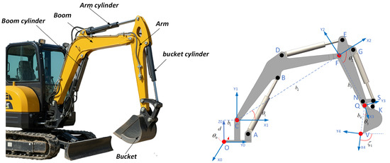
Figure 1.
D–H coordinate frame of the arm frame.
In order to verify the above technology, the parameter of a small hydraulic excavator was applied to experiments with formulaic calculations. The content of this paper is carried out without considering the rotation of the base. In the practical engineering application, it is important to solve this inverse problem because the excavator can follow a predetermined trajectory accurately. The mapping from the bucket tip’s pose to the working device’s joint angles is defined by the inverse kinematics as
where is the vector angle, respectively, between , and the horizontal plane, and counterclockwise is positive.
2.2. Hydraulic System Modeling
2.2.1. Valve-Controlled Asymmetric Hydraulic Cylinder
The working device follows a predetermined trajectory via hydraulic actuators at each joint, controlled by servo valves. Figure 2 illustrates the diagrammatic representation of the hydraulic cylinder system governed by a valve. The load flow entering the hydraulic cylinder is divided into three components: the effective flow driving piston movement, the compression flow due to the hydraulic oil’s compressibility, and the internal leakage flow. The flow continuity equation applicable to the hydraulic cylinder appears as follows:
where symbolizes the load flow rate associated with the hydraulic cylinder, indicates the extent of piston movement, and V reflects the overall volume that includes the pair of functional chambers within the cylinder. The ratio for area, denoted as , emerges from the division , with and signifying the operational surfaces of the rodless chamber and the one with the rod, respectively. Here, constitutes the effective bulk modulus linked to the hydraulic fluid, captures the pressure imposed by the load, and encompasses the aggregate leakage coefficient pertinent to the hydraulic cylinder.
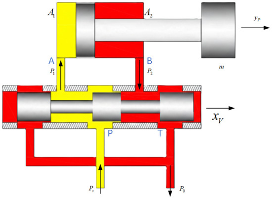
Figure 2.
Schematic of the valve-controlled hydraulic cylinder system (yellow indicates the oil inlet and red indicates the oil return).
The output flow rate of the servo valve depends on the spool displacement and the load pressure . This relationship is
where denotes the flow gain of the servo valve and is the flow–pressure coefficient of the servo valve.
The hydraulic driving force acting on the piston and the connected jib must balance the effects of inertia, viscous damping, load stiffness, and the external working load, as dictated by Newton’s second law:
where denotes the combined mass of the piston and load, represents the system’s equivalent viscous damping coefficient, specifies the equivalent spring stiffness of the load, and is the external load force.
2.2.2. Other Stage
The control signal requires electrical amplification and electro-mechanical conversion to actuate the valve spool. These components exhibit dynamic responses significantly faster than the hydraulic and mechanical parts, allowing them to be simplified as proportional components:
where denotes the overall gain from the output voltage to the spool displacement , calculated as the product of the amplifier gain and the valve gain .
2.2.3. Overall Mathematical Model of the System
By integrating Equation (3) through (6), which detail the dynamics of a single hydraulic actuator, and removing the intermediate variable , the mathematical model relating the control input to the piston displacement output, obtained via algebraic manipulation and simplification, is expressed as
where , the total flow pressure coefficient, can be noted as
where the coefficients are determined by the physical parameters of the system:
The term is defined as the lumped disturbance, which accounts for both the external load force and its rate of change.
3. Controller Design
3.1. Reference Trajectory Planning
Trajectory planning underpins high-precision trajectory tracking control. Therefore, we have formulated a complete trajectory planning scheme that consists of six major action nodes, including “contacting, cutting, scooping, lifting, discharging and returning” to guarantee the rationality and continuity of the action sequence, and it consumed 22 s in total [44].
With the aim of alleviating the repercussions arising from shifts in trajectory, we use quintic polynomial interpolation for trajectory planning at critical state points [45]. The mathematical form is as follows:
By solving the boundary conditions of every segment, coefficients of polynomial estimates are determined to make desired trajectory angle smooth in joint space. Taking advantage of the geometric property of the excavator linkage mechanism, it is converted into the exact need displacement command signals of each hydraulic cylinder, namely reference signals, as shown in Figure 3 [46].
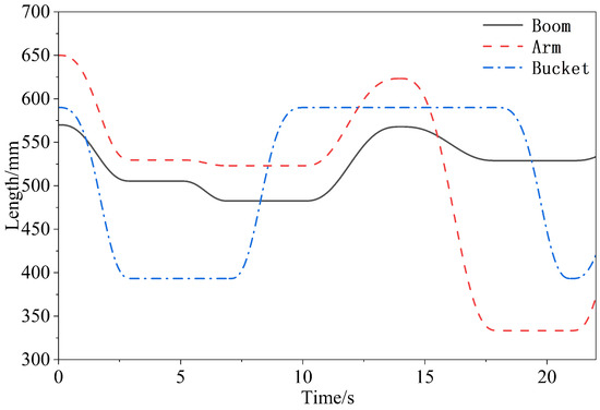
Figure 3.
Actuator planning trajectory.
3.2. Design of a Fractional-Order Adaptive Super-Twisting Sliding Mode Controller
To mitigate system uncertainties and external disturbances, the proposed controller adopts a robust feedback structure that directly uses the position tracking error. It constructs a fractional-order sliding-mode surface combined with an adaptive super-twisting algorithm to generate the control input. The corresponding control structure and methodology are illustrated in Figure 4.
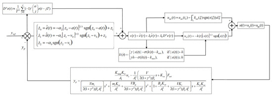
Figure 4.
Block diagram of the FO-ASTSMC control system.
First, define the position tracking error of the system:
where is the desired trajectory and is the actual displacement output of the hydraulic cylinder.
3.2.1. State Estimation Using a High-Order Sliding Mode Differentiator
To develop a second-order sliding surface for a third-order system, it is essential to determine the first derivative and the second derivative of the error. A high-order sliding mode differentiator is employed to estimate these states in real-time from [47]. The algorithm proceeds as follows:
the observations , , can converge precisely to , , in finite time. The gains , , are standard. Consequently, the state estimation values and needed by the controller are obtained.
3.2.2. Design of a Fractional-Order Sliding Surface
Conventional sliding mode controllers grounded in integer-order principles confront an inherent compromise between velocity and attenuation characteristics. Achieving rapid error convergence typically requires a higher sliding mode gain, which can lead to overshoot and oscillation, particularly in applications like hydraulic excavators under severe, time-varying conditions [48]. Conventional control laws based on instantaneous errors lose the ability to deal with persistent disturbances such as viscous soil. In order to tackle this, we apply fractional calculus theory via the incorporation of a fractional order within the architecture of the sliding surface; we equip the controller with a “memory” function to take the historical error information into account. By tuning the fractional order, the system dynamics is scalable, which makes it possible to optimize the trade-off of rapidness and dampness. The time-domain surface of the fractional-order sliding mode, which accounts for weighted integration of past errors, is formulated based on the G-L definition, giving the controller’s capability to adapt to sudden changes in load. Using this method, the moving process will have a smooth response, the chattering phenomenon can be suppressed very well, and both the tracking accuracy and stability are greatly improved. For a discrete-time system, the derivative of the error signal may be articulated in the following form:
where T is the duration of the sampling cycle, N is the memory length and stands for the binomial coefficient. The decay speed of the weight coefficients depends on the fractional-order [49]. The closer is to 1, the slower the coefficient decays, which shows that more remote error information is considered by controllers or has a stronger “memory” [50]. In engineering, selecting can achieve the optimal compromise between rapid response and smooth vibration suppression, enabling the controller to have both predictability and robustness [51].
Accordingly, the fractional-order sliding surface may be articulated in the ensuing form:
where is the coefficient of the sliding mode surface, is the fractional-order term, and an adjustable parameter can be used to balance system rapidity and the damping characteristic. When the system state approaches a sliding mode surface , then the vector scale is an ideal situation such that the solution is stable and the tracking error can be made converge to zero.
3.2.3. Design of an Adaptive Super-Twisting Control Law
Finite-time convergence to the sliding mode surface is guaranteed by the adaptive super-twisting algorithm while eliminating chattering and managing unknown disturbances. The control law is formulated as follows:
where is the nonlinear term and is the integral term. Their dynamics are defined as
where is the integral gain.
A key feature is the real-time dynamic adjustment of the controller gain , which responds to the sliding mode variable’s dynamics, thereby removing the need for prior knowledge of uncertain upper bounds. The adaptive mechanism receives its definition in the ensuing manner:
where is the adaptive rate, which controls the rise of gain. h is a small positive constant, which defines the thickness of the boundary layer. Inside this boundary layer, the control law is linearized so that the output remains smooth; outside it, a large gain rapidly suppresses proximal disturbances. is the coefficient of the bleed-off term and is used for making the gain k shrink gradually to , instead of being unbounded, while the sliding-mode variable approaches zero so that it is confined in an interval and can ensure stable and safe operation of the system. The adaptive law enables the gain k to rise swiftly, providing adequate control force when the system is distant from the sliding mode surface, and to decrease slowly when near, minimizing control energy while maintaining robustness.
3.3. System Stability Analysis
Within this segment, Lyapunov theory is used to analyze the stability of the closed-loop system under uncertainties and to establish finite-time convergence of the sliding-mode variables.
3.3.1. Problem Formulation and Sliding Mode Dynamics Derivation
Consider the third-order system model established in Section 2, which can be simplified into the following form, including lumped uncertainties composed of unmodeled dynamic external disturbances:
where F is the nominal part of the system, g is the control input gain, and is the lumped disturbance.
Assumption 1
(Convergence of the HOSM differentiator). The HOSM differentiator converges exactly in finite time . That is, for , one has and .
Assumption 2
(Bounded lumped uncertainty).
The lumped uncertainty and its time derivative are bounded. There exist unknown positive constants and such that and .
This hypothesis holds validity within physical systems. The lumped disturbance term comprises primarily two components: neglected kinetic behaviors coupled with ambiguities surrounding parametric factors, exemplified by fluctuations in the bulk modulus of hydraulic fluid, frictional dynamics, seepage within the apparatus, and extrinsic functional burdens comparable to excavation pressures. As for internal uncertainties, the ranges and magnitudes of change rates of the physical parameters associated with the system can be constrained by its own thermodynamic and hydrodynamic elements. Thus, their values and their derivatives have natural bounds. External loads are potentially very large during the excavation phase; however, their rate of change is not unbounded. The situation results from two limitations: the hydraulic system has little power, and the working device’s inertia is significantly great, which makes the external force change process physically smooth. The acting force rate of the increment is also a finite value in the case of severe working conditions, ranging from the bucket impacts.
To recap, insofar as the system is physically limited by energy, power, and mechanical inertia, it is entirely in keeping with physical reality to presume the existence of an unknown constant and such that and . Furthermore, this assumption is a classical hypothesis for designing robust controller-like sliding mode, a very common control strategy in hydraulic and robot systems.
After the differentiator converges, differentiating the fractional-order sliding surface, its dynamics can be obtained:
Substitute the system model and set :
where represents a novel total perturbation term. According to Assumption 2, it follows that is bounded; that is, an unidentified affirmative constant can be found such that holds.
Substituting the dynamics of and , the following sliding mode dynamic equations are obtained:
3.3.2. Lyapunov Stability Proof
Theorem 1.
Under Assumptions 1 and 2 in Section 3.3.1 and for controller gains satisfying and , the sliding mode dynamics (23) and (24) generated by the fractional-order sliding surface (15) and the FO-ASTSMC law (16)–(19), there exists a finite time such that, for all , the sliding variable reaches and stays on the surface . The tracking error converges asymptotically to zero.
Proof.
Select the following Lyapunov function:
the function is positive definite. It is written in the form of a quadratic form, , where the state vector is and the symmetric positive definite matrix is
Take the time derivative of V:
□
Substituting the sliding dynamics and from (23) and (24), together with the total perturbation term defined in (22), and regrouping the different contributions, one can rewrite the derivative as:
where collects the remaining terms shaped by the integral action and the adaptive law, and is a normalized disturbance term stemming from .
By Assumption 2, the lumped disturbance is bounded; hence, there exists an unknown positive constant such that .
To separate the cross terms between and v, introduce the auxiliary variable , with a positive design parameter . Using this definition, together with (25)–(27), substituting the control laws (16)–(19) into the sliding mode dynamics (23) and (24) and applying Young’s inequality to the disturbance-related terms, the derivative of the Lyapunov function can be upper-bounded as
here, are constants depending on the gains on the design parameter and on the constant g; is a small parameter related to the boundary-layer thickness h in (19); and is defined above.
Since V is quadratic in and , there exist positive constants and such that
From the upper bound in (29), it follows that . Neglecting the negative term in (28) and defining , we obtain the scalar differential inequality:
In the ideal case with a vanishing boundary layer and no external disturbance (), inequality (30) reduces to
whose solution satisfies
Implying that reaches zero in a finite time:
Therefore, and converge to zero in a finite time, and remains bounded. In the presence of bounded uncertainties (), inequality (30) shows that converges to within a small neighborhood of the origin whose size can be made arbitrarily small by choosing a thin boundary layer and operating in a regime with moderate .
Once the system trajectory enters the sliding mode (), the closed-loop motion on the manifold is governed by the fractional-order sliding dynamics , whose coefficients and are designed such that the reduced-order system is stable. This ensures that the tracking error converges asymptotically to zero. Therefore, under Assumptions 1 and 2 and under the gain conditions stated above, the closed-loop system reaches the designed second-order sliding surface in finite time, and the sliding dynamics on this surface asymptotically drive the tracking error to the origin. The asymptotic stability of the complete closed-loop arrangement is thus guaranteed.
4. Co-Simulation Results and Analysis
To evaluate the effectiveness of the proposed fractional-order adaptive super-twisting sliding mode controller (FO-ASTSMC), a unified co-simulation framework was established using AMESim 2020 and MATLAB/Simulink 2021b. The primary objective is to validate the FO-ASTSMC through comparative simulation-based performance analysis against two representative nonlinear controllers, TSMC and AFSMC. This comparative study serves two main purposes. First, it validates the effectiveness of the proposed fractional-order sliding surface in improving both dynamic response and steady-state tracking accuracy. Second, it demonstrates the advantages of the new adaptive law in terms of robustness, chattering suppression, and disturbance rejection.
4.1. Simulation Platform and Parameter Settings
The architecture of the co-simulation platform is illustrated in Figure 5. The high-fidelity excavator system, modeled in AMESim, is interfaced with controller logic operation and data exchange in Simulink. The key specifications of the system are tabulated in Table 1 and Table 2. All these parameters are determined in reference to the real small hydraulic excavator to guarantee the credibility of simulation results. It should be noted that the proposed FO-ASTSMC is validated purely through co-simulation on the AMESim–Simulink platform, without experiments on a physical excavator. Therefore, the present study mainly demonstrates the potential of the controller in a high-fidelity simulation environment, and the lack of hardware tests is a limitation that will be addressed in future work.
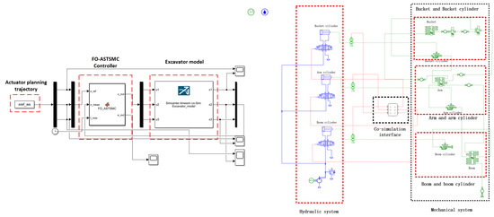
Figure 5.
Simulink–AMESim co-simulation structure of the FO-ASTSMC control system.

Table 1.
Physical parameters.
Table 2.
Hydraulic parameters.
4.2. Discussion and Results
To ensure a fair comparison, the controller parameters of FO-ASTSMC, TSMC, and AFSMC were tuned exclusively in Scenario S1 (Performance Comparison under Nominal Operating Conditions) using a common two-step procedure. First, under identical reference trajectories, sampling period, and actuator limits, a numerical optimization algorithm was used to minimize a performance index defined as a weighted sum of the root mean square error (RMSE) and maximum error (MAXE) of the three cylinders in Scenario S1. Second, starting from the optimized gains, a local search in the parameter neighborhood was conducted via repeated simulations to further reduce tracking errors while avoiding severe actuator saturation and pronounced chattering. The parameter sets obtained in Scenario S1 were then kept fixed and directly applied to Scenario S2 without any re-tuning. Consequently, the results in Scenario S2 (Robustness Comparison under Sudden Load Disturbance) primarily assess the robustness of each controller under a different operating condition.
4.2.1. Finding the Right FO Value by Tracking the Error
The optimal value for in this section is calculated by co-simulation to guarantee a normal operation for the next experiments. The range of is given above between 0 and 1. Thus, in order to determine the value of , we take 0.1, 0.5, 0.7, and 0.9. The corresponding values tracking the errors for three hydraulic cylinders are displayed in Figure 6. In this work, the fractional-order was tuned in two stages. A coarse search over , guided by the FO-SMC literature for hydraulic and robotic actuators, suggested a promising interval for the excavator hydraulic plant. Then, a fine sweep within this interval was conducted by minimizing a performance index defined as the weighted combination of RMSE and MAXE of the three cylinders under Scenario S1.
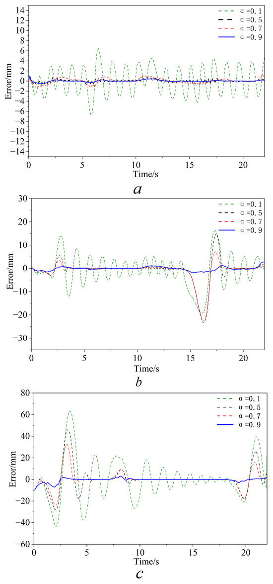
Figure 6.
FO-ASTSMC Tracking Error under Different FO(): (a) boom cylinder; (b) arm cylinder; (c) bucket cylinder.
As confirmed by the error curves in Figure 6 and the Table 3 performance plot versus , the choice yields the smallest RMSE and MAXE for all three cylinders, indicating that a larger (closer to 1) with a stronger memory effect is more suitable for the considered hydraulic plant rather than being tied to a particular trajectory.
Table 3.
Comparison of tracking performance for different fractional orders .
4.2.2. Scenario S1: Performance Comparison Under Nominal Operating Conditions
After selecting the appropriate values, juxtapose the advocated FO-ASTSMC against a duo of alternative controllers; the controller settings are as follows: , , , , , , , , , , . This scenario is performed under ideal conditions without external load perturbations and is designed to evaluate the basic tracking performance and control smoothness of each controller.
Tracking And Error Analysis: Figure 7 depicts the trajectory tracking behavior for both the controllers, operating under ideal conditions. It is clearly seen from the results that tracking curves of FO-ASTSMC coincide well with the expected trajectory, but AFSMC and TSMC have more or less overloading and oscillation. Table 4 summarizes the position tracking errors of the three controllers under the no-load condition (S1). FO-ASTSMC yields the smallest RMSE and MAXE on all three joints, whereas AFSMC shows the largest errors, and TSMC provides intermediate performance. As reported in the improvement columns of Table 4, the proposed controller reduces the average RMSE and MAXE by about and compared with AFSMC and by and compared with TSMC. These reductions suggest that the fractional-order sliding surface with memory of past errors and the adaptive super-twisting gain adjustment enhance damping and disturbance rejection, leading to improved tracking performance and steady-state accuracy over the other two schemes.
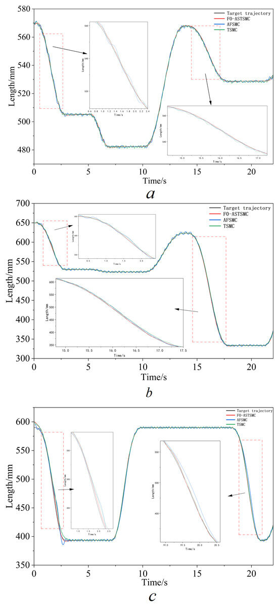
Figure 7.
Cylinder trajectory tracking results under Scenario S1: (a) boom cylinder; (b) arm cylinder; (c) bucket cylinder.
Table 4.
Comparison of controller performance indices under the nominal condition (S1).
Examination of Control Signals and Vibration Characteristics: Concurrently, a profound disparity emerges in the caliber of the control signals depicted within Figure 8. The resultant outputs from both TSMC and AFSMC exhibit pronounced high-frequency chattering, which is a typical feature of classical sliding mode designs. By contrast, the control signals generated by the proposed FO-ASTSMC are significantly smoother, confirming that the new adaptive super-twisting law effectively suppresses chattering while preserving robustness.
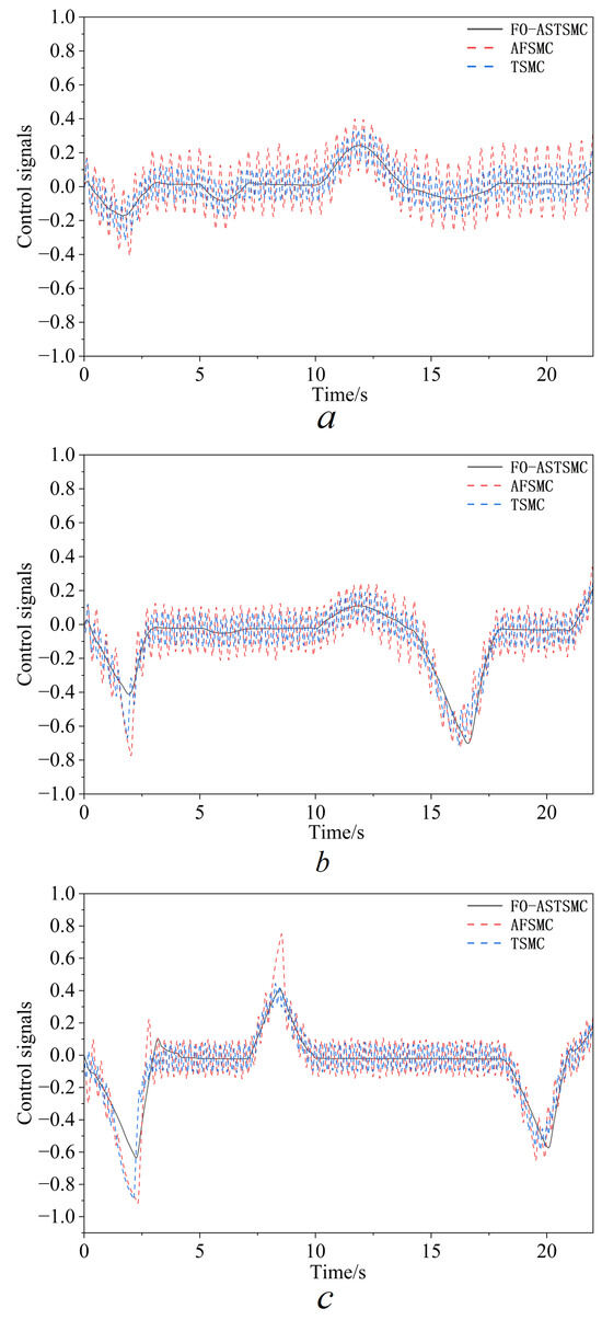
Figure 8.
Simulation results of control signals: (a) boom cylinder; (b) arm cylinder; (c) bucket cylinder.
4.2.3. Scenario S2: Robustness Comparison Under Sudden Load Disturbance
The parameters used in this section remain unchanged. This scenario simulates the time-varying loads during the excavation (7–10 s) and unloading (18–21 s) processes to rigorously test the robustness of the controller. Analysis of anti-interference and recovery performance: Figure 9 and Table 5 show the performance indicators of each controller under the condition of a sudden change in the load. Compared to the nominal condition, the FO-ASTSMC tracking curve exhibits a slight decrease from the desired trajectory, yet remains superior to the AFSMC and TSMC approaches. The AFSMC and TSMC controllers demonstrate greater delays, overshoots, and oscillations. As shown in Table 5, under the sudden-load-change condition (S2), FO-ASTSMC still attains the lowest RMSE and MAXE on all three joints, while AFSMC exhibits the largest errors and TSMC again provides intermediate performance. According to the improvement columns, the proposed controller reduces the average RMSE and MAXE by about and compared with AFSMC and by and compared with TSMC. These results indicate that the adaptive super-twisting reaching law can effectively adjust the gains online under unknown disturbance bounds and, together with the memory effect of the fractional-order sliding surface, suppresses oscillations caused by abrupt disturbances and mitigates extreme tracking errors.
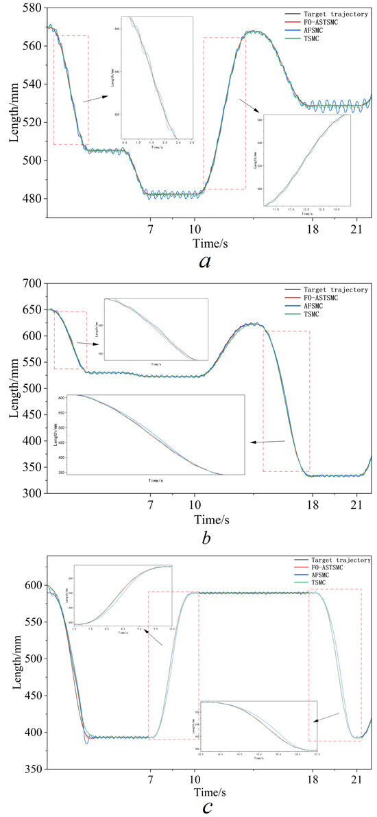
Figure 9.
Cylinder trajectory tracking results under Scenario S2: (a) boom cylinder displacement; (b) arm cylinder displacement; (c) bucket cylinder displacement.
Table 5.
Comparison of controller performance indices under the sudden-load condition (S2).
To provide an overall view of the quantitative performance, Table 6 reports the average RMSE and MAXE over the three joints, together with the percentage reductions achieved by FO-ASTSMC relative to AFSMC and TSMC under S1 and S2. It can be seen that FO-ASTSMC consistently attains the smallest average errors and the largest improvements in both scenarios. In the no-load case (S1), the proposed controller reduces the average RMSE and MAXE by about and compared with AFSMC and by and compared with TSMC. Under the sudden load-change condition (S2), the corresponding reductions reach and with respect to AFSMC and and with respect to TSMC. These results confirm that the fractional-order sliding surface with memory and the adaptive super-twisting reaching law jointly enhance damping and disturbance rejection, leading to robust tracking accuracy across different operating conditions.
Table 6.
Comparative performance analysis of different controllers under the same conditions.
Control Output and Chattering Analysis: Figure 10: the signals a, b, and c denote the respective responses of the boom, arm, and bucket during digging operation in case S1. In parallel, d, e, and f represent the corresponding signals for these components under the conditions of case S2. Figure 11: panels a, b, and c depict the signals corresponding to the boom, arm, and bucket throughout the unloading stage within scenario S1; meanwhile, d, e, and f convey the signals for the boom, arm, and bucket across the unloading span in scenario S2. The comparison of loads between boom, arm, and bucket for the control systems’ outputs during excavation and material unloading is presented. This value also reinforces our analysis above. The actual responses of TSMC and AFSMC all have severe fluctuations when the loading operation is performed. Although FO-ASTSMC’s output voltage varies in comparison with the no-load operation, it still provides high smoothness compared with the other two controllers. This indicates that the good chattering-suppression ability of the excavator working device is not restricted to ideal working conditions but is also valid under severe working conditions.
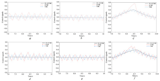
Figure 10.
Control signals of the boom, arm, and bucket during the digging operation in cases S1 and S2: (a–c) boom, arm, and bucket in case S1; (d–f) boom, arm, and bucket in case S2.
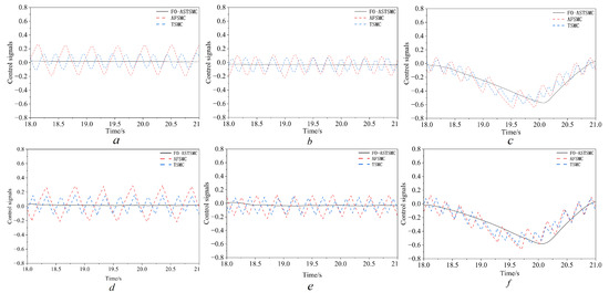
Figure 11.
Control signals of the boom, arm, and bucket during the unloading stage in cases S1 and S2: (a–c) boom, arm, and bucket in case S1; (d–f) boom, arm, and bucket in case S2.
The above results of the simulation in this chapter also validate the two primary innovations of the proposed FO-ASTSMC controller. 1. Utilizing fractional-order calculus within the sliding mode surface design empowers the suggested controller to attain marked advancements in tracking accuracy (RMSE) under typical scenarios, outperforming the reference techniques. 2. Under the sudden load-change condition, through application of the new adaptive super-twisting law, strong disturbance-suppression capability is revealed, compared with traditional methods, which can effectively restrain the transient peak error (MAXE) and then guarantees the robustness of system stability. The overall controller’s performance is a breakthrough for both innovations together, as indicated in the complete data. That is, high accuracy and the excellent stability and anti-interference performance make FO-ASTSMC an effective means of solving the problem of how to achieve high-accuracy hydraulic servo control.
4.3. Practical Implementation Considerations
While this study is primarily verified through simulation, the proposed control strategy is designed with practical implementation constraints in mind. From a hardware deployment perspective, the FO-ASTSMC requires only position measurements of the boom, arm, and bucket cylinders. These signals are readily available in standard electro-hydraulic systems via LVDT or magnetostrictive sensors, eliminating the need for additional costly instrumentation.
Regarding real-time performance, a sampling period of 1–2 ms (500–1000 Hz) is sufficient to capture the dominant dynamics of the valve-controlled cylinders. Furthermore, the computational load—including the fractional-order sliding surface, high-order sliding differentiator, and adaptive laws—is kept compatible with mid-range industrial controllers or embedded PCs (e.g., execution times within tens of microseconds per cycle in benchmarking). Consequently, the FO-ASTSMC algorithm can be readily integrated into existing electro-hydraulic servo architectures by replacing the conventional PID module while retaining the original sensors and valve drivers. Detailed hardware implementation and experimental validation on a scaled excavator prototype are planned for future work.
5. Conclusions
In light of strong nonlinearity, uncertain parameters, and sudden load changes in practice, a FO-ASTSMC to deal with working-device trajectory tracking for small hydraulic excavators is developed to enhance accuracy and robustness. The proposed controller combines the memory capability of fractional calculus, the continuous robust control feature of the super-twisting algorithm, and the online parameter tuning mechanism of an adaptive law, and it applies a high-order sliding-mode differentiator for state estimation. The controller can operate without speed sensors, which may reduce hardware costs. Based on Lyapunov stability theory, we provide a rigorous proof that the proposed controller ensures finite-time convergence of the sliding-mode variables and guarantees asymptotic stability in the presence of lumped uncertainties and external disturbances. Co-simulation results in AMESim and Simulink indicate that, under nominal working conditions, FO-ASTSMC achieves smaller RMSE and maximum error than the benchmark controllers at every joint. Under sudden load changes, the proposed method also exhibits improved suppression of the peak tracking error and smoother control signals. These results suggest that the FO-ASTSMC has the potential to provide high-precision, robust, and actuator-friendly control for hydraulic excavators; however, the present validation is limited to AMESim–Simulink co-simulation, and experimental verification on a physical prototype is left for future work. In future studies, the control scheme will also be extended to multi-joint coordinated control in Cartesian space.
Author Contributions
Conceptualization, S.Z. and Z.L.; methodology, S.Z., M.L. and D.L.; software, S.Z.; validation, S.Z. and M.L.; investigation, S.Z. and M.L.; data curation, S.Z., M.L., C.W. and H.L.; writing—original draft, S.Z. and M.L.; writing—review and editing, S.Z. and M.L. All authors have read and agreed to the published version of the manuscript.
Funding
This research was supported by the National Natural Science Foundation of China Grant (51765014) and the Natural Science Foundation of Guangxi Grant (2025GXNSFAA069959).
Institutional Review Board Statement
Not applicable.
Informed Consent Statement
Not applicable.
Data Availability Statement
The original contributions presented in this study are included in the article; further inquiries can be directed to the corresponding author.
Acknowledgments
The authors would like to thank the editor and the anonymous reviewers for their constructive comments and suggestions that helped improve the quality of this manuscript.
Conflicts of Interest
The authors declare no conflicts of interest.
References
- Zhang, L.; Zhao, J.; Long, P. An autonomous excavator system for material loading tasks. Sci. Robot. 2021, 6, eabc3164. [Google Scholar] [CrossRef] [PubMed]
- Asama, H. Remote-Controlled Technology and Robot Technology for Accident Response and Decommissioning of Fukushima Nuclear Power Plant. Insights Concern. Fukushima Daiichi Nucl. Accid. 2021, 2, 199–208. [Google Scholar]
- Eraliev, O.M.U.; Lee, K.H.; Shin, D.Y. Sensing, perception, decision, planning and action of autonomous excavators. Autom. Constr. 2022, 141, 104428. [Google Scholar] [CrossRef]
- Feng, H.; Jiang, J.; Chang, X. Adaptive sliding mode controller based on fuzzy rules for a typical excavator electro-hydraulic position control system. Eng. Appl. Artif. Intell. 2021, 126, 107008. [Google Scholar] [CrossRef]
- Fu, T.; Zhang, T.; Lv, Y.; Song, X.; Li, G.; Yue, H. Digital Twin-Based Excavation Trajectory Generation of Uncrewed Excavators for Autonomous Mining. Autom. Constr. 2023, 149, 10482. [Google Scholar] [CrossRef]
- Wang, J.; Zhang, H.; Hao, P.; Deng, H. Observer-Based Approximate Affine Nonlinear Model Predictive Controller for Hydraulic Robotic Excavators with Constraints. Processes 2023, 11, 1918. [Google Scholar] [CrossRef]
- Phan, V.D.; Ahn, K.K. Fault-tolerant control for an electro-hydraulic servo system with sensor fault compensation and disturbance rejection. Nonlinear Dyn. 2023, 111, 10131–10146. [Google Scholar] [CrossRef]
- Li, J.; Li, W.; Du, X. Research on the characteristics of electro-hydraulic position servo system of RBF neural network under fuzzy rules. Sci. Rep. 2024, 14, 15332. [Google Scholar] [CrossRef]
- Yuan, X.; Wang, W.; Zhu, X. Theoretical model of dynamic bulk modulus for aerated hydraulic fluid. Chin. J. Mech. Eng. 2022, 35, 121. [Google Scholar] [CrossRef]
- Jose, J.T.; Das, J.; Mishra, S.K.; Wrat, G. Early detection and classification of internal leakage in boom actuator of mobile hydraulic machines using SVM. Eng. Appl. Artif. Intell. 2021, 106, 104492. [Google Scholar] [CrossRef]
- Zhang, T.; Yan, G.; Liu, X. Nonlinear flow modeling of electro hydrostatic pump unit based on Gauss Newton iterative method for high performance control. Sci. Rep. 2024, 14, 21750. [Google Scholar] [CrossRef]
- Zhou, R.; Meng, L.; Yuan, X. Experimental Test and Feasibility Analysis of Hydraulic Cylinder Position Control Based on Pressure Detection. Processes 2022, 10, 1167. [Google Scholar] [CrossRef]
- Chen, M.; Si, L.; Dai, J. A variable structure robust control strategy for automatic drilling tools loading and unloading system. Control Eng. Pract. 2025, 161, 106340. [Google Scholar] [CrossRef]
- Yu, S.; Song, X.; Sun, Z. On-line prediction of resistant force during soil–tool interaction. J. Dyn. Syst. Meas. Control 2023, 145, 081004. [Google Scholar] [CrossRef]
- Sun, Y.; Wang, Y.; Wang, L. Digging Performance and Stress Characteristic of the Excavator Bucket. Appl. Sci. 2023, 13, 11507. [Google Scholar] [CrossRef]
- Won, D.; Kim, W.; Tomizuka, M. Nonlinear Control With High-Gain Extended State Observer for Position Tracking of Electro-Hydraulic Systems. IEEE/ASME Trans. Mechatron. 2020, 25, 2610–2621. [Google Scholar] [CrossRef]
- He, Z.; Jiang, B.; Sun, C. Electro-hydraulic position servo system based on sliding mode active disturbance rejection compound control. Proc. Inst. Mech. Eng. Part C J. Mech. Eng. Sci. 2022, 236, 2089–2098. [Google Scholar] [CrossRef]
- He, J.; Su, S.; Wang, H. Online PID tuning strategy for hydraulic servo control systems via sac-based deep reinforcement learning. Machines 2023, 11, 593. [Google Scholar] [CrossRef]
- Wu, L.; Liu, J.; Vazquez, S. Sliding mode control in power converters and drives: A review. IEEE/CAA J. Autom. Sin. 2022, 9, 392–406. [Google Scholar] [CrossRef]
- Mousavi, Y.; Bevan, G.; Küçükdemiral, I.B. Sliding mode control of wind energy conversion systems: Trends and applications. Renew. Sustain. Energy Rev. 2022, 167, 112734. [Google Scholar] [CrossRef]
- Sun, C.; Dong, X.; Wang, M.; Li, J. Sliding Mode Control of Electro-Hydraulic Position Servo System Based on Adaptive Reaching Law. Appl. Sci. 2022, 12, 6897. [Google Scholar] [CrossRef]
- Soon, C.C.; Ghazali, R.; Ghani, M.F. Chattering analysis of an optimized sliding mode controller for an electro-hydraulic actuator system. J. Robot. Control 2022, 3, 160–165. [Google Scholar] [CrossRef]
- Xu, R.; Wang, Z.; Zhou, M. A robust fractional-order sliding mode control technique for piezoelectric nanopositioning stages in trajectory-tracking applications. Sens. Actuators A Phys. 2023, 363, 114711. [Google Scholar] [CrossRef]
- Dong, H.; Yang, X.; Kuang, Z. On practical terminal sliding-mode control for systems with or without mismatched uncertainty. J. Frankl. Inst. 2022, 359, 8084–8106. [Google Scholar] [CrossRef]
- Hou, Q.; Ding, S. Finite-time extended state observer-based super-twisting sliding mode controller for PMSM drives with inertia identification. IEEE Trans. Transp. Electrif. 2022, 8, 1918–1929. [Google Scholar] [CrossRef]
- Choi, A.; Kim, H.; Hu, M. Super-Twisting Sliding Mode Control with SVR Disturbance Observer for PMSM Speed Regulation. Appl. Sci. 2022, 12, 10749. [Google Scholar] [CrossRef]
- Lao, L.; Chen, P. Adaptive sliding mode control of an electro-hydraulic actuator with a Kalman extended state observer. IEEE Access 2024, 12, 8970–8982. [Google Scholar] [CrossRef]
- Tho, N.H.; Phuong, V.N.Y.; Danh, L.T. Development of an Adaptive Fuzzy Sliding Mode Controller of an Electrohydraulic Actuator Based on a Virtual Prototyping. Actuators 2023, 12, 258. [Google Scholar] [CrossRef]
- Tao, X.; Liu, K.; Yang, J. Sliding Mode Backstepping Control of Excavator Bucket Trajectory Synovial in Particle Swarm Optimization Algorithm and Neural Network Disturbance Observer. Actuators 2025, 14, 9. [Google Scholar] [CrossRef]
- Guo, X.; Wang, H.; Liu, H. Adaptive Sliding Mode Control with Disturbance Estimation for Hydraulic Actuator Systems and Application to Rock Drilling Jumbo. Appl. Math. Model. 2024, 136, 115637. [Google Scholar] [CrossRef]
- Deng, W.; Yao, J.; Wang, Y. Output feedback backstepping control of hydraulic actuators with valve dynamics compensation. Mech. Syst. Signal Process. 2021, 158, 107769. [Google Scholar] [CrossRef]
- Ding, H.; Wang, Y.; Zhang, H. Robust output feedback position control of hydraulic support with neural network compensator. Actuators 2023, 12, 263. [Google Scholar] [CrossRef]
- Ruderman, M. Extended fractional-order jeffreys model of viscoelastic hydraulic cylinder. J. Dyn. Syst. Meas. Control 2021, 143, 074502. [Google Scholar] [CrossRef]
- Hui, J.; Yuan, J. Chattering-free higher order sliding mode controller with a high-gain observer for the load following of a pressurized water reactor. Energy 2021, 223, 120066. [Google Scholar] [CrossRef]
- Zhu, P.; Chen, Y.; Li, M.; Zhang, P.; Wan, Z. Fractional-order sliding mode position tracking control for servo system with disturbance. ISA Trans. 2020, 105, 269–277. [Google Scholar] [CrossRef]
- Yang, X.; Yao, J.; Deng, W. Output feedback adaptive super-twisting sliding mode control of hydraulic systems with disturbance compensation. ISA Trans. 2021, 109, 175–185. [Google Scholar] [CrossRef]
- Wan, Z.; Fu, Y.; Yue, L.; Liu, C. Adaptive super-twisting sliding mode control of hydraulic servo actuator with nonlinear features and modeling uncertainties. Stroj. Vestn.–J. Mech. Eng. 2022, 68, 771–780. [Google Scholar] [CrossRef]
- Xie, Y.; Zhang, X.; Meng, W.; Zheng, S.; Jiang, L.; Meng, J.; Wang, S. Coupled fractional-order sliding mode control and obstacle avoidance of a four-wheeled steerable mobile robot. ISA Trans. 2021, 108, 380–391. [Google Scholar] [CrossRef]
- Jing, C.; Zhang, H.; Liu, Y.; Zhang, J. Adaptive super-twisting sliding mode control for robot manipulators with input saturation. Sensors 2024, 24, 2783. [Google Scholar] [CrossRef]
- Zhang, S.; Li, Z.; Wang, H.N.; Xiong, T. Fractional Order Sliding Mode Control Based on Single Parameter Adaptive Law for Nano-Positioning of Piezoelectric Actuators. IET Control Theory Appl. 2021, 15, 1422–1437. [Google Scholar] [CrossRef]
- Barros, L.C.D.; Lopes, M.M.; Pedro, F.S. The memory effect on fractional calculus: An application in the spread of COVID-19. Comput. Appl. Math. 2021, 40, 72. [Google Scholar] [CrossRef]
- Yang, X.; Chen, W.; Yin, C. Fractional-order sliding-mode control and radial basis function neural network adaptive damping passivity-based control with application to modular multilevel converters. Energies 2024, 17, 580. [Google Scholar] [CrossRef]
- Razzaghian, A.; Kardehi, M.R.; Pariz, N. Disturbance observer-based fractional-order nonlinear sliding mode control for a class of fractional-order systems with matched and mismatched disturbances. Int. J. Dyn. Control 2021, 9, 671–678. [Google Scholar] [CrossRef]
- Jin, Z.; Gong, M.; Zhao, D.; Luo, S.; Li, G.; Li, J.; Zhang, Y.; Liu, W. Mining Trajectory Planning of Unmanned Excavator Based on Machine Learning. Mathematics 2024, 12, 1298. [Google Scholar] [CrossRef]
- Zhang, Y.; Sun, Z.; Sun, Q. Time-jerk optimal trajectory planning of hydraulic robotic excavator. Adv. Mech. Eng. 2021, 13, 16878140211034611. [Google Scholar] [CrossRef]
- Ding, H.; Sang, Z.; Li, Z. Trajectory planning and control of large robotic excavators based on inclination-displacement mapping. Autom. Constr. 2024, 158, 105209. [Google Scholar] [CrossRef]
- Wetzlinger, M.; Reichhartinger, M.; Horn, M. Higher order sliding mode inspired nonlinear discrete-time observer. Syst. Control Lett. 2021, 155, 104992. [Google Scholar] [CrossRef]
- Filo, G. Artificial intelligence methods in hydraulic system design. Energies 2023, 16, 3320. [Google Scholar] [CrossRef]
- Yavuz, M.; Öztürk, M.; Yaskıran, B. Sliding Mode Controller of Fractional Order for a Robot Manipulator Control. In Proceedings of the International Conference on Computational Modeling and Sustainable Energy, Gandhinagar, India, 15–17 December 2023; pp. 193–213. [Google Scholar]
- Rodríguez-Mata, A.E.; Medrano-Hermosillo, J.A.; López-Pérez, P.A. A novel fractional high-order sliding mode control for enhanced bioreactor performance. Fractal Fract. 2024, 8, 607. [Google Scholar] [CrossRef]
- Chaudhary, K.S.; Kumar, N. Fractional Order Fast Terminal Sliding Mode Control Scheme for Tracking Control of Robot Manipulators. ISA Trans. 2023, 142, 57–69. [Google Scholar] [CrossRef]
Disclaimer/Publisher’s Note: The statements, opinions and data contained in all publications are solely those of the individual author(s) and contributor(s) and not of MDPI and/or the editor(s). MDPI and/or the editor(s) disclaim responsibility for any injury to people or property resulting from any ideas, methods, instructions or products referred to in the content. |
© 2025 by the authors. Licensee MDPI, Basel, Switzerland. This article is an open access article distributed under the terms and conditions of the Creative Commons Attribution (CC BY) license (https://creativecommons.org/licenses/by/4.0/).