Article

Fault Prediction Method Towards Rolling Element Bearing Based on Digital Twin and Deep Transfer Learning

1
College of Communication Engineering, Chongqing Polytechnic University of Electronic Technology, Chongqing 401331, China
2
School of Information Engineering, China University of Geosciences, Beijing 100083, China
*
Author to whom correspondence should be addressed.
Appl. Sci. 2025, 15(23), 12509; https://doi.org/10.3390/app152312509
Submission received: 12 October 2025 / Revised: 10 November 2025 / Accepted: 19 November 2025 / Published: 25 November 2025

Abstract

Rolling element bearing failure in industrial robots can cause system downtime, high repair costs, and significant economic losses. Traditional fault diagnosis methods assume that training and testing data follow the same distribution, requiring extensive historical data, which is often impractical in dynamic operational environments. Digital twin and transfer learning technologies offer a new approach for intelligent fault diagnosis, addressing these limitations. This paper combines model knowledge and data-driven approaches using digital twin and transfer learning for bearing fault diagnosis. First, a dynamic twin model of the bearing is developed using MATLAB/Simulink (R2018a), simulating fault data under various operating conditions that are difficult to obtain in real-world scenarios. A multi-level construal neural network algorithm is then proposed to minimize cumulative errors in data preprocessing. The digital twin technology generates a balanced dataset for pre-training the model, which is subsequently applied to real-time fault diagnosis in industrial robot bearings via transfer learning, bridging the gap between virtual and physical entities. Experimental results demonstrate the feasibility of the method, with a diagnostic accuracy of 96.95%, marking a 15% improvement over traditional convolutional neural network methods without digital twin enhancement.

1. Introduction

Rolling element bearings (REBs) operate under complex and variable conditions, and their operating environment is harsh [1]. They are susceptible to failures in the inner and outer rings, as well as rolling elements, due to various influencing factors, which in turn affect the performance and efficiency of the equipment. Deep learning, which can adaptively extract features from source data, has gradually been applied to the field of intelligent fault diagnosis [2]. REB faults are often sporadic, and the data collected by online monitoring equipment exhibit characteristics such as non-stationarity, non-linearity, and low signal density [3]. Additionally, building experimental platforms to collect data samples has certain limitations, making it difficult to simulate all types of faults and fault severities. As a result, the number of fault samples for various REB faults is relatively small and highly imbalanced compared to normal data, which makes it challenging to support the large sample sizes required for deep learning-based fault diagnosis methods. Furthermore, the instability of REB data under varying operating conditions leads to differences in feature distributions between the training and testing datasets, which reduces the generalization ability of diagnostic models and lowers the fault diagnosis accuracy under variable operating conditions [4].
Previous research on REB fault diagnosis has primarily focused on vibration signals collected from REBs [5]. Based on the developmental trajectory, these methods can be classified into two categories: shallow machine learning methods based on signal analysis and deep learning methods. In shallow machine learning methods based on signal analysis, features of the collected REB vibration signals are first extracted and selected using time-frequency analysis, and then pattern recognition is performed using shallow machine learning algorithms, such as extreme learning machines. These methods heavily rely on manual feature extraction and expert knowledge from the domain, which significantly limits their effectiveness. Deep learning-based REB fault diagnosis methods, on the other hand, utilize deep neural network structures to perform layer-wise feature extraction of the input samples, thereby achieving automatic feature extraction and eliminating reliance on manual and domain expert inputs [6]. However, the traditional REB fault diagnosis methods described above largely depend on a large number of labeled samples and assume that the training and testing datasets follow the same data distribution, which is not suitable for the real-world applications of industrial robots, where fault samples are scarce, imbalanced, and require online state diagnosis.
The emergence of digital twin (DT) and transfer learning technologies perfectly addresses the limitations of traditional REB fault diagnosis methods, providing new solutions and methodologies for fault prediction and prognostics health management in industrial robots. DT technology enables bi-directional interaction between virtual entities and physical entities, thereby facilitating online condition monitoring and fault diagnosis [7]. Additionally, DT models can generate a large amount of sample data without loss, solving the imbalance problem caused by small sample sizes in the actual production of wind turbines. Transfer learning breaks the conventional assumption in traditional machine learning that the training and testing datasets must have the same data distribution [8]. It leverages knowledge learned from one task or domain to improve learning performance in another task or domain, significantly reducing learning time and costs for new tasks and enhancing the accuracy and efficiency of knowledge acquisition [9]. Therefore, the study of a novel intelligent fault diagnosis method for industrial robot REBs from the perspective of combining DT and transfer learning is a trending direction in the field of industrial robot fault diagnosis, with high academic and practical value for real-world industrial robots.
Currently, some research on DT models remains in the theoretical stage, with the latest achievements in DT models only able to simulate partial REB states [10]. This paper proposes a fusion model that combines model knowledge and data-driven approaches for industrial robot REB fault diagnosis. This model applies DT-based fault diagnosis to industrial robot REBs for the first time, simulating the complete state of the REBs using a dynamic twin model, and implementing an end-to-end fault diagnosis model based on parameter transfer learning for raw vibration signals. This method not only avoids errors and technical requirements in the data preprocessing stage of traditional methods but also effectively solves the challenges of insufficient and imbalanced data in industrial robots. Particularly, compared to the high cost and risk of obtaining REB fault data through physical damage experiments, this technological framework provides a safe, reliable, and low-cost alternative solution.
The remainder of this paper is organized as follows. Section 2 reviews existing studies on deep transfer learning and DT. Section 3 presents the design of a DT-assisted deep transfer learning algorithm. Section 4 presents a case study of REBs based on the DT-assisted deep transfer learning algorithm. Section 5 provides an interpretation of the results. Finally, Section 6 concludes the paper and discusses future work.

2. Related Works

2.1. Deep Transfer Learning-Based Fault Prediction

Wang et al. presented a deep transfer learning framework that enhances failure prediction performance across different failure types by leveraging knowledge transfer in data-scarce conditions [11]. Chen et al. provided a systematic review of deep transfer learning applications in REB fault diagnosis since 2016, highlighting its effectiveness in improving fault detection and classification across various scenarios [12]. Yan et al. offered a comprehensive survey on the use of deep transfer learning for anomaly detection in industrial time series, exploring methods, applications, and future research directions to improve fault prediction in industrial settings [13]. Xiang et al. proposed a micro transfer learning mechanism for cross-domain equipment remaining useful life (RUL) prediction, aiming to enhance prediction accuracy by transferring knowledge between different domains with limited data [14]. Zheng et al. introduced a meta-transfer learning-based method for multi-fault analysis and assessment in power systems, aiming to improve fault prediction and diagnosis by transferring knowledge across different fault scenarios [15]. Zheng et al. presented an unsupervised transfer learning method combining structure-optimized convolutional neural networks and fast batch nuclear-norm maximization for REB fault diagnosis, enhancing fault detection by transferring knowledge without requiring labeled data [16]. Pathak et al. explored a deep learning-based approach for defect detection in film-coated tablets using a convolutional neural network, aiming to improve the accuracy of identifying defects in pharmaceutical manufacturing [17]. Y Azad et al. developed a deep learning-based method for autonomous morphological fracture analysis of fiber-reinforced composites, leveraging deep learning techniques to accurately predict and analyze material fractures [18].
A deep transfer learning model with high fault prediction accuracy is achieved when it leverages both source and target domain knowledge effectively. If the domain gap between source and target data is too large, the model may fail to generalize well, leading to reduced prediction performance. The limited generalization ability is an inherent challenge in deep transfer learning. To improve fault diagnosis accuracy, the deep transfer learning model should be incorporated into a comprehensive diagnostic system, enabling better fault detection across varied operating conditions.

2.2. DT-Based Fault Prediction

He et al. presented a two-stage updated DT model for predicting the remaining useful life of REBs, enhancing the accuracy of fault prediction by continuously updating the DT with real-time data [19]. Rana et al. provided a systematic review of artificial intelligence (AI)-driven fault detection and predictive maintenance in electrical power systems, focusing on data-driven approaches, DTs, and self-healing grids to improve fault prediction and system reliability [20]. Mikołajewska et al. explored the integration of generative AI in AI-based DTs for fault diagnosis and predictive maintenance, enhancing predictive accuracy and decision-making in Industry 4.0/5.0 environments [21]. Sun et al. presented a fault diagnosis method for proton exchange membrane fuel cell systems by combining DT technology with unsupervised domain adaptive learning, improving fault detection across different operating conditions [22]. Gong et al. proposed a DT-assisted intelligent fault diagnosis approach for REBs, leveraging real-time data and advanced analytics to enhance fault detection and prognosis accuracy [23]. Ye et al. developed a data-driven digital twin architecture for failure prediction in customized automatic transverse robots, utilizing real-time data to enhance predictive maintenance and system reliability [24]. Yin et al. introduced a DT-driven approach for fault identification in distribution networks connected to distributed wind power, improving fault detection and system resilience through real-time monitoring and simulation [25]. Xue et al. presented a DT-driven fault diagnosis method for CNC machine tools, enhancing fault detection and maintenance by integrating real-time data and predictive analytics [26].
The traditional DT model for REB fault prediction often relies on idealized operating conditions, which may not reflect the actual performance of the REB, resulting in discrepancies and reduced prediction accuracy. To address this, this paper integrates sensor data with a multi-level construal neural network (MLCNN) to enhance the DT model’s ability to predict REB faults more accurately. This approach improves the fault diagnosis precision and extends the predictive maintenance capabilities of REBs.

3. The Proposed Method

3.1. DT Model

The concept of DT was first introduced by Grieves [27]. In general, a DT refers to a digital replica created for an actual device or system, which is known as the DT entity. The DT entity exists in the virtual world of an information platform, integrating data such as physical models, offline historical data, real-time sensor data, and model storage. It combines interdisciplinary knowledge, multidimensional physical attributes, details at different scales, and probabilistic analysis to implement a highly realistic simulation process. By building high-fidelity simulations, the DT can precisely map and dynamically update the state of its physical counterpart in a virtual environment, enabling comprehensive tracking and simulation of the evolution of the physical device throughout its lifecycle. DT technology tightly integrates advanced information technologies and digital modeling techniques. Through the interaction between the physical object and its virtual representation, it can depict the multidimensional characteristics, behaviors, and current state of the object in detail, and predict and analyze its future evolution. This technology provides practical solutions for monitoring, simulating, predicting, and optimizing physical entities and fulfilling functional service and application needs.
For common fault defects in industrial robot REBs, a five-degree-of-freedom dynamic model using MATLAB-Simulink (R2018a) is established based on the method in [28], as shown in Figure 1. In this REB model, the rotor is driven at a constant speed, and the model has five degrees of freedom. The outer and inner rings each have two degrees of freedom, and another degree of freedom is introduced due to an added spring-mass system to represent high-frequency resonant vibrations. In Figure 1, M P , K P , and R P represent the mass, stiffness, and damping of the base, respectively; M S , K S , and R S represent the mass, stiffness, and damping of the rotor shaft with the inner ring, respectively; and M R , K R , and R R represent the mass, stiffness, and damping of the spring-mass system.
The following assumptions are made for the model: The outer ring of the REB is fixed, and the inner ring rotates at a constant speed. The contact between the rolling bodies and the outer ring, as well as the contact between the rolling bodies and the inner ring, is defined as surface contact, following Hertz’s contact theory. Contact loads are generated only when the rolling bodies are in rolling contact with the inner or outer rings. The mass of the rolling bodies is neglected, they are equally spaced at angular intervals, and both the rolling bodies and the cage rotate at a constant angular velocity. All translational motions occur within the x-y plane, and rotation occurs along the z-axis.
The azimuthal angle θ j of the j-th rolling element at t moment can be expressed as follows [29]:
θ j = 2 π j 1 n b + w c t + θ 0
where n b is the total number of rolling bodies, θ 0 is the initial azimuthal angle of the first rolling element, j is an integer from 1 to b n , and w c is the angular frequency of the cage rotation, expressed as follows [29]:
w c = w i 2 1 d D
where d and D are the pitch diameter of the REB and the diameter of the rolling element, respectively, and w i is the angular frequency of the inner ring, rad/s.
The j-th rolling elements in the horizontal direction are given by the Hertzian contact force Equations (3) and (4). Here, γ is the load-deformation exponent ( γ ball   bearing = 3/2, γ roller   bearing = 10/9).
K b is the load coefficient of the rolling element.
F x = j = 1 n b K b δ j γ cos θ j h δ j
F y = j = 1 n b K b δ j γ cos θ j h δ j
The Heaviside function can be expressed as follows [29]:
h x = 1 , x 0 0 , x < 0
When the REB is in a normal state, the contact deformation δ j of the j-th rolling element with a radial clearance H can be expressed as follows:
δ j = x d cos θ j + y d sin θ j H
where x d and y d are the relative displacements of the REB inner ring, REB inner ring, and rolling element in the x-direction and y-direction, respectively. When δ j < 0 , the contact force disappears, and traction or friction forces are not modeled in the five-degree-of-freedom model.
Considering the non-linear contact stiffness, the system’s motion differential equations are represented by Equations (7)–(11).
M P x ¨ 0 = F x R P x ˙ 0 K P x 0
M P y ¨ 0 = F y M P g R P + R R y 0 K P + K R y 0 + K R y R + R R y ˙ R
M s x ¨ i = F x + R s x ˙ i + K S x i
M S y ¨ i = F y M S g R S y ˙ i K S y i
M R y ¨ R = K R y 0 y R + R R y ˙ 0 y ˙ R M R g
where F x and F y represent the contact forces; x o and y o represent the displacement of the external center of mass; x i and y i represent the displacement of the inner ring center of mass; y R represents the displacement of the spring-loaded mass system; and g represents the gravitational acceleration.
For this five-degree-of-freedom model, the base mass and stiffness are adjusted to match the system’s low natural frequencies (obtained from modal testing), and the spring-mass system’s stiffness and damping are chosen to excite the typical high-frequency resonant response of the REB (15 kHz, 5% damping).

Local Fault Modeling

Local faults are modeled following the method described in [28].
(1)
Outer Ring Fault
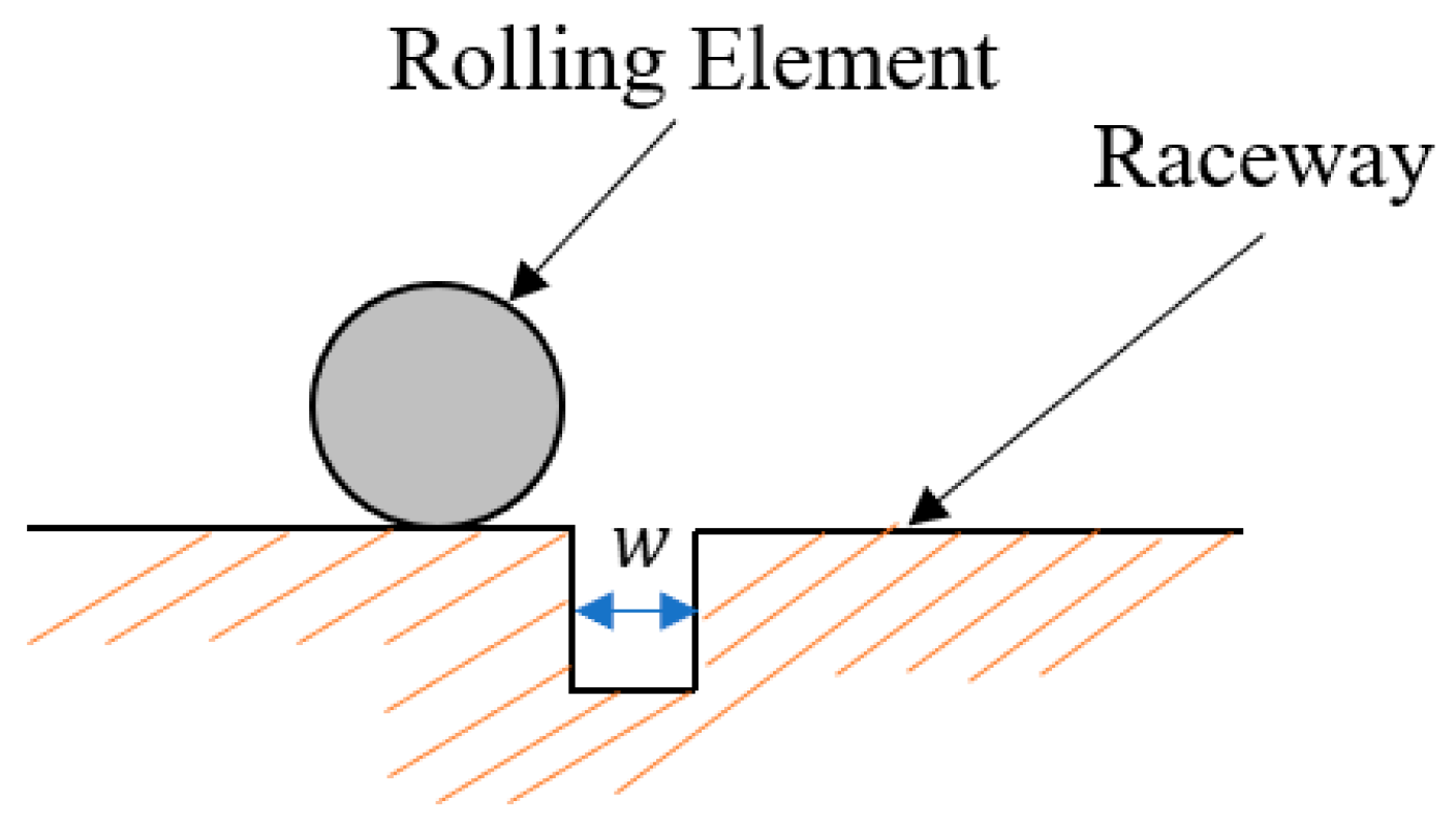
The outer ring fault is modeled as a small rectangular spall on the raceway, as shown in Figure 2.
When a rolling element approaches a specific angular position ϕ d , it enters the spalling region, where the contact force suddenly disappears; when it leaves the spalling region, the contact force is restored. These contact losses and gains generate a large number of periodic pulse forces. The contact deformation under outer ring fault can be expressed as follows [29]:
δ o = max x d cos θ j + y d sin θ j H δ f , 0
where δ f = C d , ϕ d < θ j < ϕ d + Δ ϕ d 0 , o t h e r ; x d = x i x o ; y d = y i y o ; Δ ϕ d = 2 w D o ; C d represents the change in displacement of the rolling element due to the movement of the spalled layer.
(2)
Inner Ring Fault
The modeling approach for inner ring failure is similar to that of outer ring failure described above. When inner ring failure occurs, the debris rotates with the inner ring, causing its position to change continuously. Therefore, the value of ϕ d depends on the rotational angle of the rotor shaft, and can be expressed as follows [29]:
ϕ d = w i t + ϕ 0
where ϕ 0 is the initial position of the spalling, and the corresponding contact deformation is given by the following [29]:
δ i = max x d cos θ j + y d sin θ j H δ f , 0
where δ f = C d , ϕ d < θ j < ϕ d + Δ ϕ d 0 , o t h e r .
(3)
Rolling Element Fault
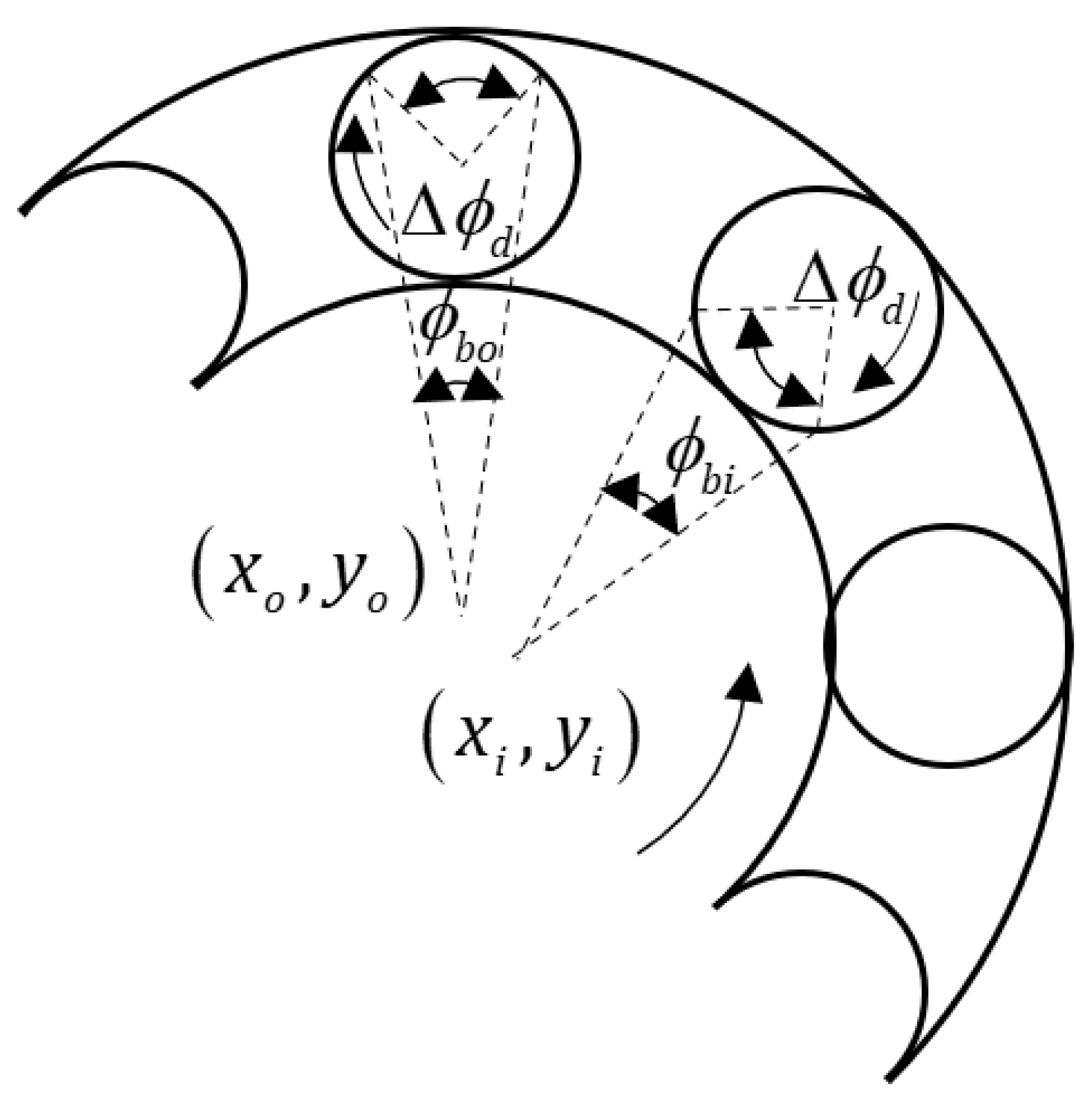
The spalled debris on the rolling element rotates at the same speed as the rolling element. At any given time, the angular position of the spalled debris (as shown in Figure 3) is represented by the angular position ϕ s of the rolling element spall, expressed as follows [29]:
ϕ s = w i D 2 d 1 d D cos ϕ 2 t + ϕ 0
where ϕ 0 is the initial position of the spall, and the rotational direction of the rolling element is opposite to the rotor shaft’s direction of rotation.
For rolling element faults, the angular widths of the spalled areas on the inner and outer rings are illustrated in Figure 3 and can be expressed as follows [29]:
ϕ b i = Δ ϕ d d / D i
ϕ b o = Δ ϕ d d / D o
where D i and D o are the inner and outer diameters of the REB, respectively; D = D i + D o / 2 .
δ f is given by the following [29]:
δ f = C d = C d r C d o , 0 < ϕ s < ϕ b C d r + C d i , 0 < ϕ s < π + ϕ b i 0 , o t h e r
where C d r represents the distance by which the rolling element moves upward from its original contact position due to the spalling area; C d i represents the maximum depth of the inner ring entering the spalling area when the rolling element makes contact with the inner ring; and C d o represents the displacement of the outer ring, which can be expressed as follows [29]:
C d r = 1 2 d d 2 4 x 2
C d r = 1 2 D i D i 2 4 x 2
C d o = 1 2 D o D o 2 4 x 2
The contact deformation under rolling element failure can be expressed as follows [29]:
δ j = max x d cos θ j + y d sin θ j H δ f , 0

3.2. MLCNN

The MLCNN is designed to enhance model performance by providing multi-level interpretations of data, making it capable of handling complex, multi-faceted data and learning representations at different abstraction levels [30]. The core idea is to use hierarchical layers of interpretation that allow the network to progressively refine its understanding of the data through different levels of abstraction. This technique enables the network to achieve better generalization and robustness, especially in domains with complex or noisy data. Therefore, the MLCNN is suitable for the fault prediction of REB.
The MLCNN uses multiple layers, where each layer represents a different level of construal (interpretation). The first layer interprets raw input data at a low level, the middle layers work on more abstract representations, and the last layers aim for high-level reasoning and decision-making. Each layer in the MLCNN refines the features it receives from the previous layer by applying learned transformations, enhancing data representation progressively. The architecture is designed to enable the flow of information across multiple abstraction levels. At each level of construal, the network learns not only the local features of the input but also how to interpret these features in context. This allows for better performance on tasks requiring contextual understanding and reasoning. The MLCNN incorporates a multi-level loss function that encourages the network to minimize errors at each abstraction level. This ensures that the network focuses on learning both low-level features and high-level interpretations simultaneously.
Let x be the input data, and y be the desired output. The network consists of L layers, with each layer l represented by a transformation function f l · .
For each layer l , the input data is transformed as follows [30]:
h l = f l h l 1 , W l , b l
where h l 1 is the input to the l -th layer (with h 0 = x ), W l is the weight matrix for the l -th layer, b l is the bias term for the l -th layer, and f l · is the transformation function (e.g., convolution, activation function).
The overall loss function L combines the errors from each abstraction level [30]:
L = l = 1 L λ l L l h l , y
where L l h l , y is the loss at layer l , and λ l is the weight factor for the loss at layer l .
The final output of the network is computed by the last layer L [30]:
y ^ = f L h L 1 , W L , b L
The prediction error is the difference between the predicted output y ^ and the true output y [30]:
E r r o r =   y ^   - y
The network adjusts its parameters W l and b l during training to minimize this error using backpropagation.

3.3. DT-Assisted Deep Transfer Learning Method

3.3.1. Problem Description

Given two different domains and learning tasks, namely the source domain D S and learning task T S , and the target domain D T and learning task T T , transfer learning aims to improve the learning of the target task D T by leveraging the knowledge from both the source domain D S and learning task T S , D S D T . The challenge of transfer learning lies in reducing the discrepancy between the source domain D S and target domain D T . Therefore, this paper defines a hybrid prediction for deep transfer learning assisted by DTs. The problem is described as follows: for a given set of M fault categories and N S samples X S = x i i = 1 N S in the source domain, the corresponding labels are denoted by Y S = y i i = 1 N S , where y i 0 , 1 , , M 1 . Similarly, for the given number of M fault categories and N t samples X t = x i i = 1 N t in the target domain, the corresponding labels are denoted by Y t = y i i = 1 N t , where y i 0 , 1 , , M 1 . The source domain dataset for the proposed model is D S = x i , y i i = 1 N S , and the target domain dataset is D t = x i , y i i = 1 N t . This paper constructs a series of tasks A 1 n to evaluate, and during the source domain subset screening, the weight coefficients of the corresponding samples are calculated using the class diversity matrix and distance constraint matrix of the source domain samples X S , ensuring the removal of the impact of negative samples.

3.3.2. Model Structure

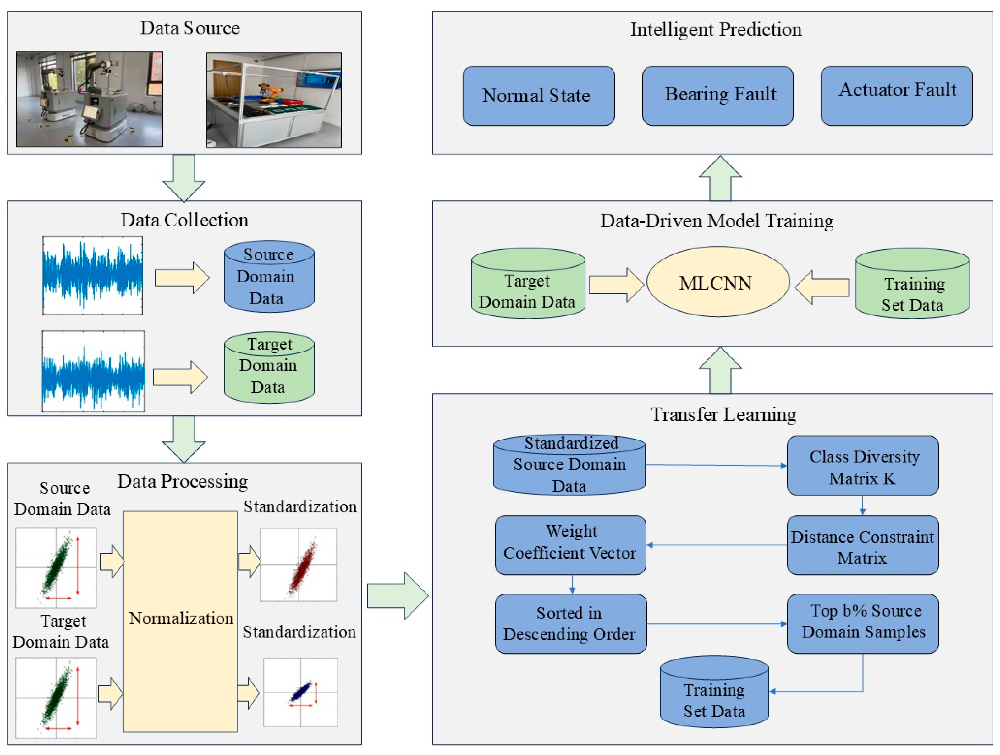
Figure 4 shows the structure of the intelligent prediction model for deep transfer learning assisted by DTs, which includes data collection, data processing, deep transfer learning algorithms, data-driven model training, and intelligent prediction.
Data Collection: In this study, the collected industrial robot REB data is analyzed in the time-frequency domain. Through numerous comparative experiments, the corresponding dimensions for transferring fault types and samples are determined, and the sample datasets for the source and target domains are constructed.
Data Processing: The data processing section uses Min-Max normalization to eliminate dimensional influence x 1 , x 2 , , x n . The sequence is transformed, and standardized source and target domain datasets are constructed.
Deep Transfer Learning: The data weight of the source domain is restricted using the class diversity matrix K and distance constraint matrix W , ensuring that the selected samples include all classes in the source domain and maintain appropriate distances between the samples. The parameters of the deep transfer learning model include p c t , R 1 , and R 2 , where p c t represents the proportion of selected samples from the source domain, and R 1 and R 2 represent the weights of the class diversity matrix K and distance constraint matrix W , respectively. Grid search is used to optimize these hyperparameters, and the training samples are arranged in descending order of the weight coefficient vector.
Typically, there are two situations that lead to classification errors in the target domain. The first case is when the selected data points do not contain all the classes from the source domain, and the second case is when the selected data points are a non-distance subset, i.e., the selected data points are too close to each other. To eliminate the impact of negative samples and accurately classify the target domain, class-balanced information and a discriminative subset need to be selected.
In the deep transfer learning model assisted by DTs, if x i and x j belong to the source domain and share the same class label, the value of k i , j will be 1. x i and x j should not be selected as representatives simultaneously. If x i is chosen as the representative, then x j should be removed. Therefore, this study selects class-balanced information and a discriminative subset. The elements k i , j of the class diversity matrix K are calculated as follows:
k i , j = 1 , x l i = x l j 0 , x l i x l j
The distance constraint matrix W ensures the selection of a diverse representative subset. Unlike the class diversity matrix K , the design of the matrix W is inspired by clustering concepts. The elements w i , j of matrix W are computed by calculating the local distance between data points x i and x j in the source domain:
w i , j = 1 ,   i f   x i N p x j   o r   x j N p x i 0 , o t h e r w i s e
where x i N p x j indicates that x i is one of the k nearest neighbors of x j . In this study, the parameter is set to 5 to obtain k nearest neighbors. For example, if x i and x j are sufficiently close, then w i , j = 1. To ensure the diversity of the selected samples, x i and x j should not be chosen simultaneously.
The weight coefficient vector α corresponding to the source domain sample is obtained through iterative optimization, and the source domain data is sorted in descending order using the Sortrows function to select the sample subset with the highest weight coefficients.
Data-Driven Model: In this study, the MLCNN is selected as the classifier for the experiment, and the training set after removing negative samples is used to train the classifier to accomplish the classification task for the target domain.

3.3.3. Optimization Objective

In transfer learning, effective methods are needed to minimize the distribution discrepancy between D S and D T . The Maximum Mean Discrepancy (MMD) is the most commonly used loss function in transfer learning to model the distribution discrepancy between the source and target domains. The Reproducing Kernel Hilbert Space (RKHS) is a mathematical structure for handling function spaces, widely used in machine learning, statistics, and signal processing. The projection matrix maps the data from both the source and target domains into the RKHS, and the difference in means between D S and D T in the common subspace is computed. The equation is given as follows:
min P 1 n s i = 1 n s P T x i s 1 n t j = 1 n t P T x j t 2 s . t .     P T P = I
To perform transfer learning using Equation (29), it is necessary to determine whether all data from the source domain is beneficial for the transfer process. In practical applications, some source domain samples exhibit deviations from the target domain samples, which hinder the reduction in the distribution discrepancy between the source and target domains. If all data from the source domain is selected directly, negative transfer issues may arise.
In deep transfer learning, there is a large amount of labeled data in the source domain for training the source domain model. In the target domain, a small amount of data is selected through active learning for labeling, and the target domain model is constructed by combining the source and target domain data. Deep transfer learning aims to select the most informative target domain samples to reduce the bias between the source and target domains. Therefore, this study extends and minimizes MMD in deep transfer learning to select appropriate source domain samples.
min P   M M D F 2 D S , D T , P = 1 S i = 1 S P T x i s 1 t j = 1 t P T x j F 2 s . t .       P T P = I
To select appropriate samples in the source domain, this paper defines α as the weight coefficient for source domain data x i , and α = α 1 , α 2 , , α s T R s × 1 as the overall weight coefficient vector. By weighting the source domain data α , the distribution of the source domain data is adjusted. It is assumed that the higher the weight α i , the greater the probability that the corresponding data point x i will be selected. Therefore, the MMD is reformulated as follows in Equation (31):
min P , α   M M D F 2 D S , D T , P , α = 1 S i = 1 S P T x i α i 1 t j = 1 t P T x j F 2 s . t . P T P = I , i = 1 s α i = 1 , α i 0 , x i D S , y j D T
where F 2 represents the Frobenius norm of a matrix, abbreviated as the F-norm. i = 1 S α i = 1 and α i 0 are constraints imposed to avoid arbitrary scaling of α i . The core problem of Equation (31) is to select appropriate samples that minimize the probability distribution difference between D S and D T .
For deep transfer learning models, if x i and x j come from the source domain and share the same class label, then the value of k i , j is 1. In this case, these two data points should not be selected as representatives simultaneously. If x i is selected as a representative, then x j should be discarded. Thus, the paper selects class-balanced information and a discriminative subset. To maintain the above assumption, the following function is minimized to make the selected data points as diverse as possible.
i = 1 S j = 1 S α i α j k i , j
The distance constraint matrix W is derived from the local distance relationship between the source domain data points x i and x j , where x i N k ( x j ) indicates that x i is one of the k nearest neighbors of x j . Setting the parameter k = 5 results in the matrix W . If x i and x j are close enough, W i , j = 1 . To ensure the diversity of selected samples, x i and x j should not be selected together. Therefore, at least one of α i and α j must have a small value. The function to minimize is formulated as follows:
i = 1 S j = 1 S α i α j w i , j
In summary, the optimization function for the entire deep transfer learning model is given as follows:
min P , α   L P , α = 1 S i = 1 S P T x i α i 1 t j = 1 t P T y j H 2 + λ 1 i = 1 S j = 1 S α i α j k i , j + λ 2 i = 1 S j = 1 S α i α j k i , j s . t .   P T P = I , i = 1 S α i = 1 , α i 0
where λ 1 0 ,   λ 2 0 represent the importance of weight parameters for K and W , respectively, α i weight the importance of x i positions and determine whether x i can be selected as representatives. In other words, if α i has a high value, the corresponding data point is selected. Therefore, this paper sorts α i in descending order and selects the data points with high α i values.
Based on this, the paper designs a DT-assisted deep transfer learning algorithm, and the pseudocode is shown in Algorithm 1.
Algorithm 1. Pseudocode for DT-assisted deep transfer learning algorithm
1. Initialize Source domain data X s , Target domain data X t , Matrix weights R 1 , R 2 , Maximum iteration count i max and set values   α =   0 ,   P   =   1 a 2 + b 2 , v   =   0 ,   y 1   = 0 ,   y 2   =   0 ,   μ   = 0.1 ,   μ m a x   = 105 ,   i   = 1
2. Calculate the class diversity matrix K using Equation (27)
3. Calculate the distance diversity matrix W using Equation (28)
4. While  i < i max
5. Normalize the source domain samples f e a t u r e s n s and input them, using the Adam algorithm to solve for the weight parameters
6. α 2 n S 2 X S T P P T X S + λ 1 K + K T + λ 2 W + W T + 2 μ I S I S T 1 × 2 s t X S T P P T X t I t + μ I S y 1 I S + μ v y 2
7. Λ p 1 S 2 X S α α T X S T 2 S t X S α α T X S T + 1 t 2 X t I t I t T X t T p
8. v = max 0 , α + 1 μ y 2
9. y 1 = y 1 + μ α T I s I y 2 = y 2 + μ α v μ = min ρ μ , μ max
10. Sort the source domain data in descending order based on the weight coefficient vector
11. Select the top b% of the data to form the training set
12. Input the training set data X S = F e a s × P
13. Use grid search to optimize the hyperparameters
14. Diagnose the target domain data and obtain the final fault status
15. Compare with the original labels and calculate the diagnosis accuracy
16. End

3.3.4. Intelligent Prediction Process

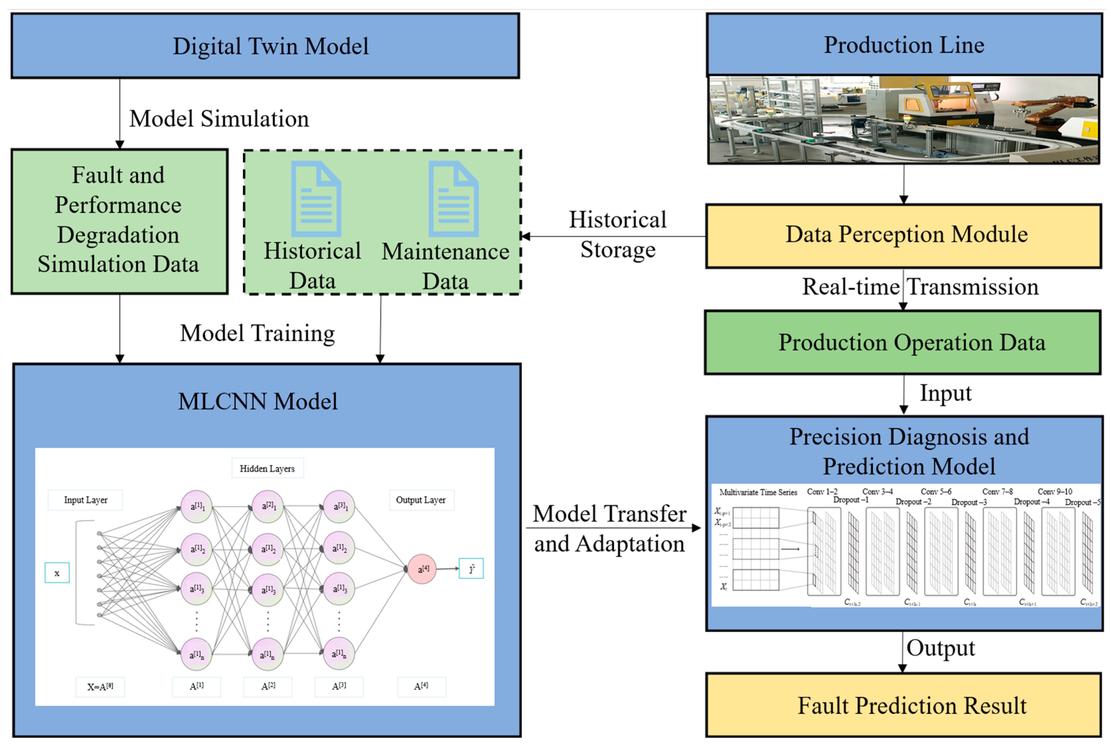
Figure 5 presents the intelligent prediction process assisted by DTs and deep transfer learning. Deep transfer learning transfers knowledge from the source domain DT model to the target domain MLCNN data-driven model, enabling diagnostic and predictive tasks in scenarios with difficult-to-label data, such as industrial robot REB fault diagnosis and remaining useful life prediction. In this study, this paper first establishes a DT model for key production line equipment. This model uses mathematical relationships to describe the physical properties of the equipment and generates simulated fault data. The MLCNN data-driven model is then trained, and through deep transfer learning, the trained MLCNN model is transferred to actual fault data to obtain accurate prediction results. The DT-assisted deep transfer learning algorithm utilizes the theoretical values from the DT-driven model to correct the actual values of the MLCNN data-driven model. The specific process of Algorithm 1 is as follows:
(1)
State Space Model Transformation: Based on the performance degradation laws of the DT model, the state transformation is performed, calculating the internal state of the DT system and generating fault simulation data.
(2)
Construction of MLCNN-Based Data-Driven Model: The source domain data is used to train the MLCNN model, enabling data feature learning and fault prediction.
(3)
Deep Transfer Learning Algorithm: Knowledge from the source domain DT model is transferred to the target domain MLCNN data-driven model. During the transfer learning process, the model parameters are adjusted to adapt to the characteristics of the target domain data, thereby improving the model’s generalization ability.
(4)
Intelligent Prediction Analysis: Based on the intelligent prediction results from DT-assisted deep transfer learning, the predicted value is analyzed to determine if it exceeds the threshold. If the threshold is exceeded, maintenance operations are performed; otherwise, the process returns to step 2 for iteration.

4. Case Study

4.1. Experimental Platform Setup

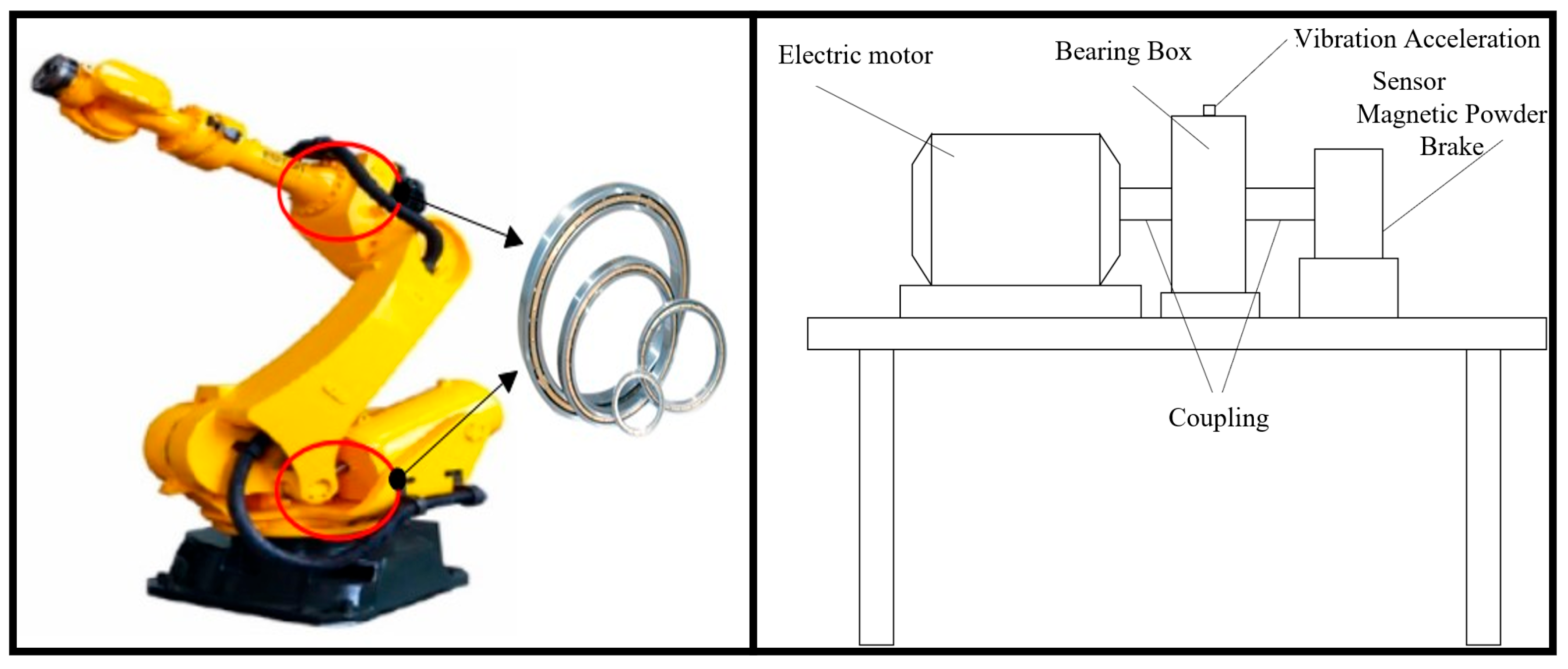
In the actuator of industrial robots, the REB is a critical component with a high failure rate. Therefore, this paper proposes a REB fault prediction method based on deep transfer learning. The industrial robot model is the ABB IRB120 robotic arm. Figure 6 illustrates the REB fault prediction experimental platform. The motor provides power to the platform, which is connected to the REB box via a coupling. The REB box is braked by a magnetic powder brake. A vibration acceleration sensor is installed on the REB box to collect REB vibration data. Table 1 shows the REB fault data.
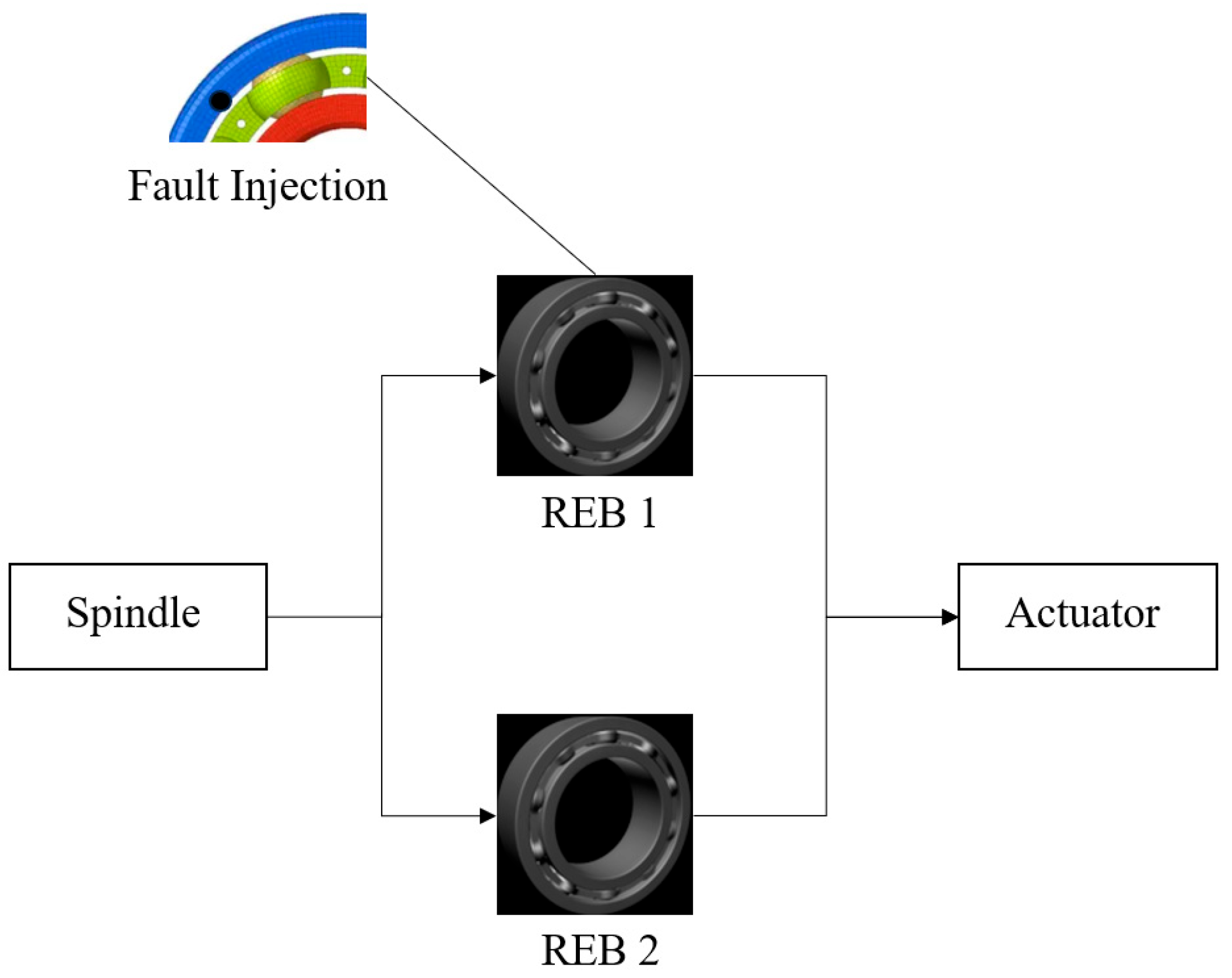
In the REB fault prediction experiment, manual damage to the REB is required, and data acquisition calibration takes a long time, making REB fault prediction less feasible. Therefore, this paper simulates fault data based on the DT model of the REB and uses the obtained simulated fault data to train the MLCNN data-driven model. After training, the MLCNN data-driven model is transferred to the actual REB working environment for fault prediction through deep transfer learning.

4.2. Construction of the REB DT Model and Fault Injection

In this paper, the DT model of the REB is set with faults, including the outer ring, inner ring, and rolling element faults, and fault injection is completed in the simulation model. Figure 7 shows the DT model of the REB, where REB faults are artificially injected as pitting on the DT geometric model.
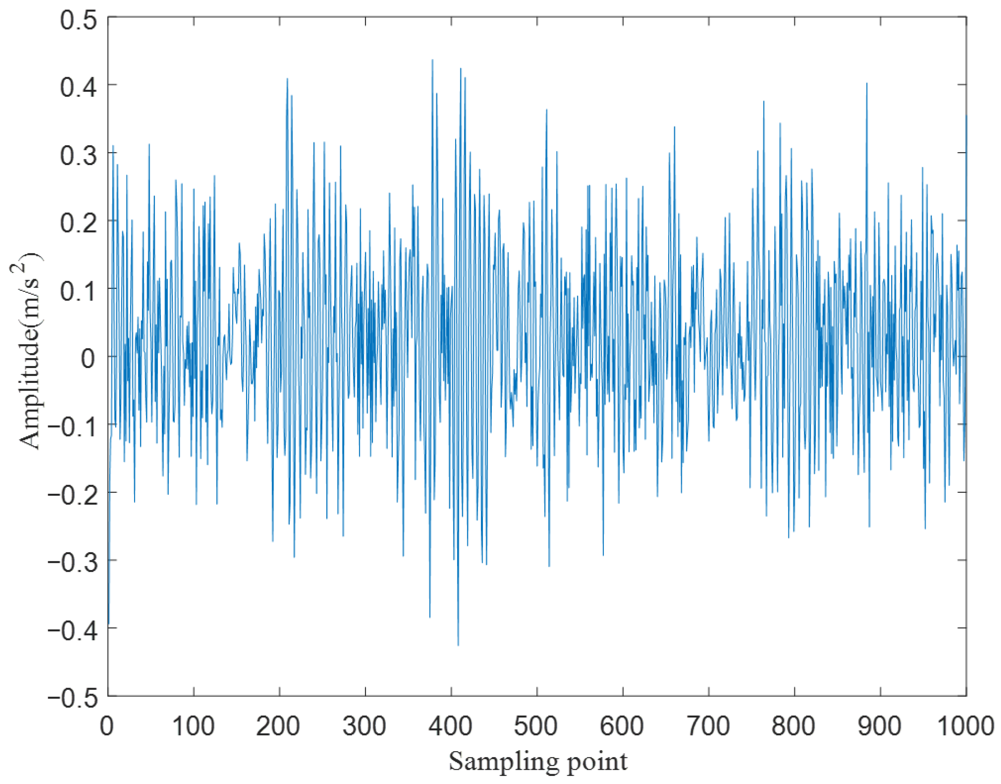
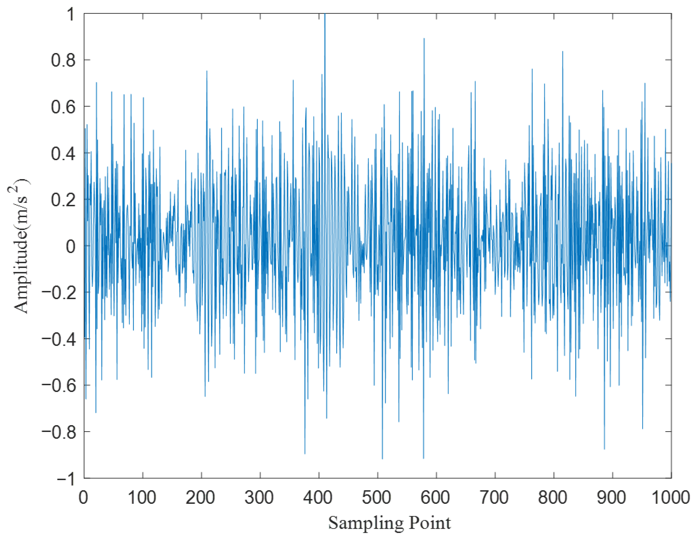
The DT model of the REB includes a vibration acceleration sensor added to the model to collect simulated vibration signals from the DT model. This study simulates the vibration signals of the REB at speeds ranging from 400 to 700 rpm/min. Figure 8 shows the simulated vibration signal of the REB at 700 rpm/min in the DT model.

4.3. Construction of MLCNN Data-Driven Model and Actual Fault Transfer

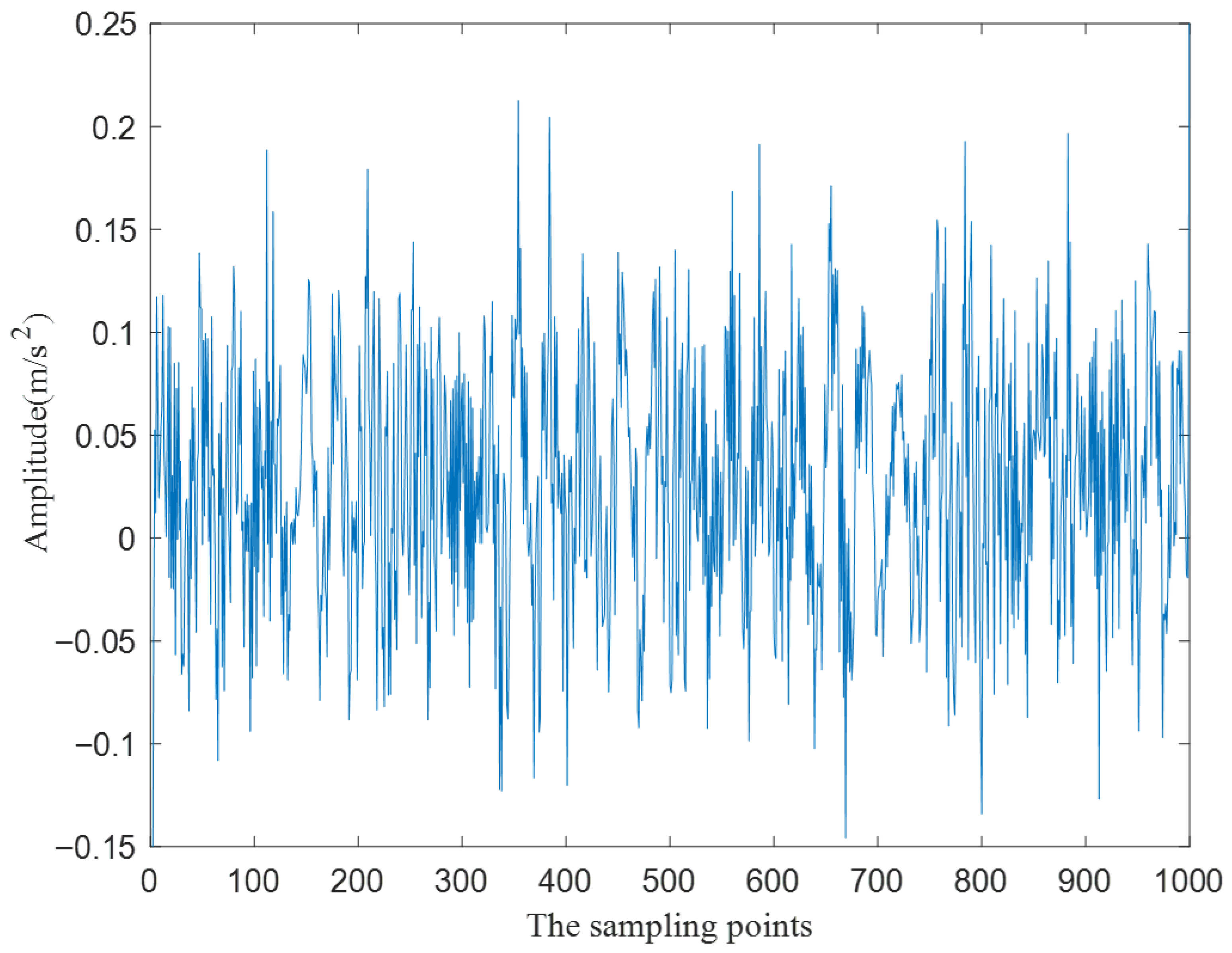
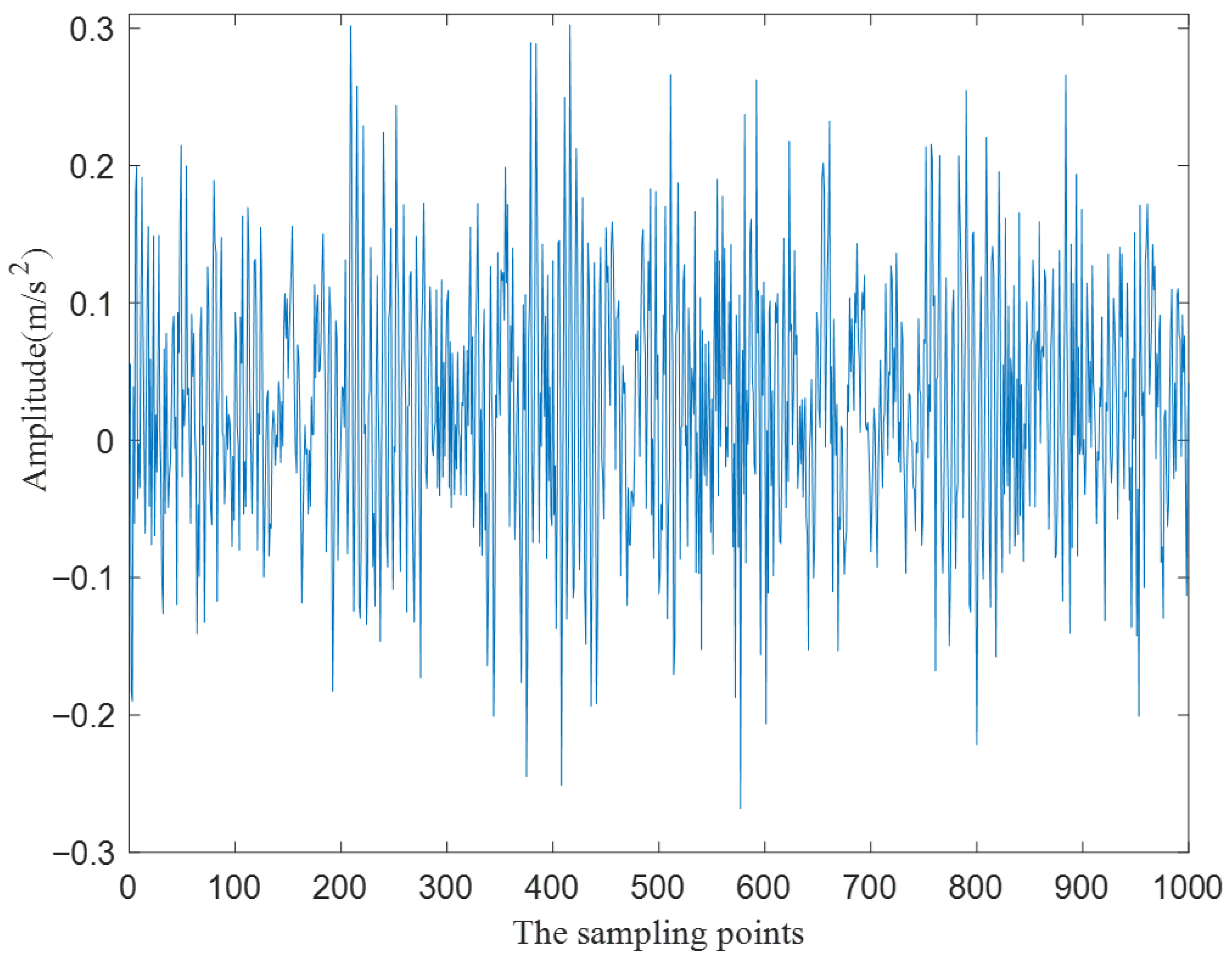
In this paper, the simulated bearing data is smoothed to effectively eliminate noise. Figure 8 shows the bearing simulation signal, which contains a significant amount of noise. To reduce computational complexity, a moving average filter is applied for smoothing, and the results are shown in Figure 9. The moving average filtering method is detailed in [4]. The smoothed data is split into 70% for the training set and 30% for the testing set. Finally, the data is standardized and normalized using the Z-score normalization method and the min-max normalization method, as described in [6].
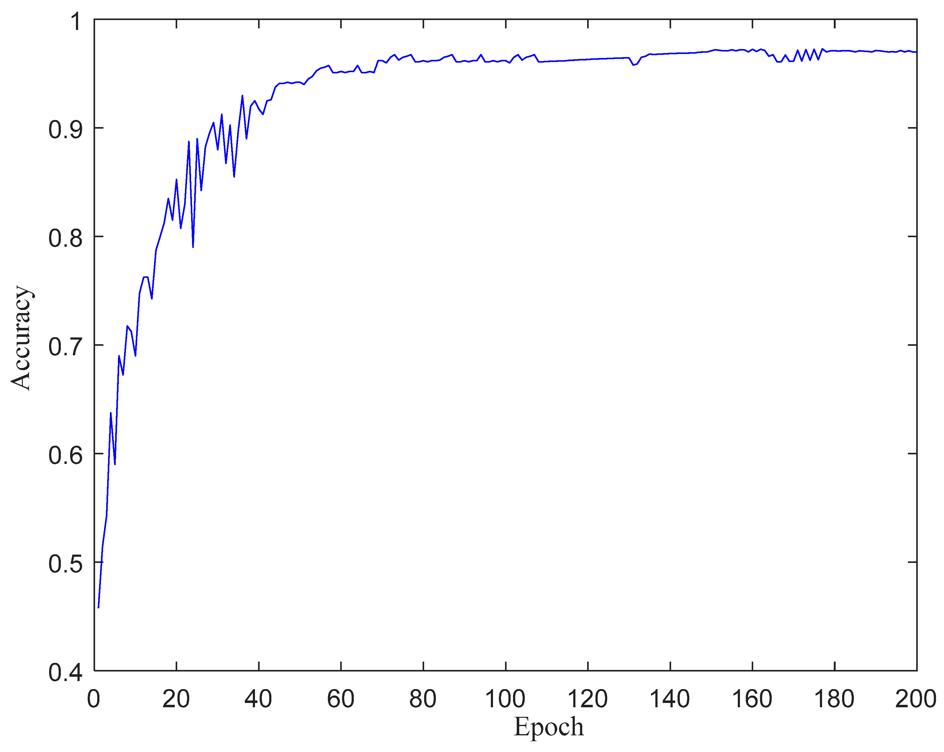
The simulation data for the REB in the DT model consists of 12 working conditions. This paper constructs a one-dimensional MLCNN data-driven model to predict REB faults. The parameters for the MLCNN model are as follows: the input layer consists of 512 sample data points, three convolutional layers and ReLU activation layers, one pooling layer and Softmax layer, and the output layer is set to 12. The input layer is set to 512 data points, reflecting the typical duration of fault signals in the dataset. Three convolutional layers are chosen based on prior research, offering an ideal balance between capturing both local and global features without introducing unnecessary complexity. ReLU activation functions are used for their ability to mitigate the vanishing gradient problem and improve training efficiency. A single pooling layer is included to reduce dimensionality and prevent overfitting while focusing on the most significant features of the data. The Softmax layer in the output layer is employed to convert raw outputs into a probability distribution for multi-class classification. The chosen hyperparameters are validated through a grid search. Figure 10 shows the training results of the simulated fault data from the DT model, with a fault prediction accuracy of 97%. This performance reflects an effective balance between model complexity and generalization.
The fault prediction at 700 rpm/min is verified as an example. With known speed, only four REB fault states need to be predicted. The MLCNN data-driven model, trained with the simulated data from the DT model, is transferred to actual REB fault data through deep transfer learning. Figure 10 shows the actual REB fault data.
Table 2 compares the actual vibration signal of the REB at 700 rpm/min with the DT simulated signal. Based on data feature analysis, the error between the actual vibration signal and the DT simulated signal is minimal, maintaining the high fidelity of the DT model.
The actual bearing data collected in this study is also smoothed to effectively remove noise. Figure 11 depicts the bearing simulation signal, which contains substantial noise. To minimize computational complexity, the moving average filter is employed for smoothing, with the processing results shown in Figure 12. The moving average filtering method is detailed in [4]. The smoothed data is divided into 70% for the training group and 30% for the testing group. Finally, the data is standardized and normalized using the Z-score standardization method and the min-max normalization method [6].
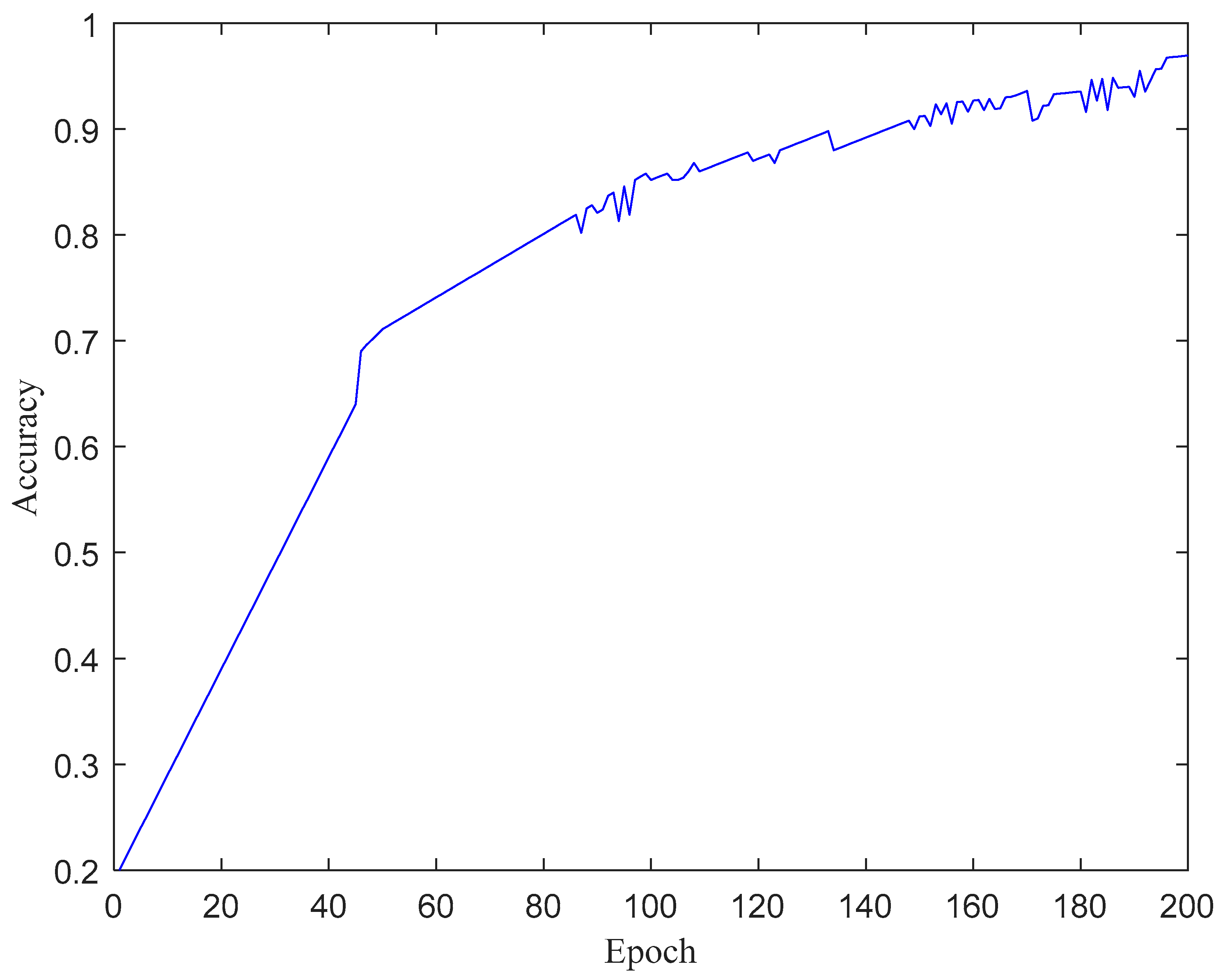
By modifying the Softmax layer and output layer of the MLCNN algorithm, the output categories are set to 4. Figure 13 presents the intelligent prediction results based on deep transfer learning. The fault signals simulated by the DT model train the MLCNN data-driven model, which is then transferred to actual fault signals for fault prediction. The fault prediction accuracy reaches 96.95%.
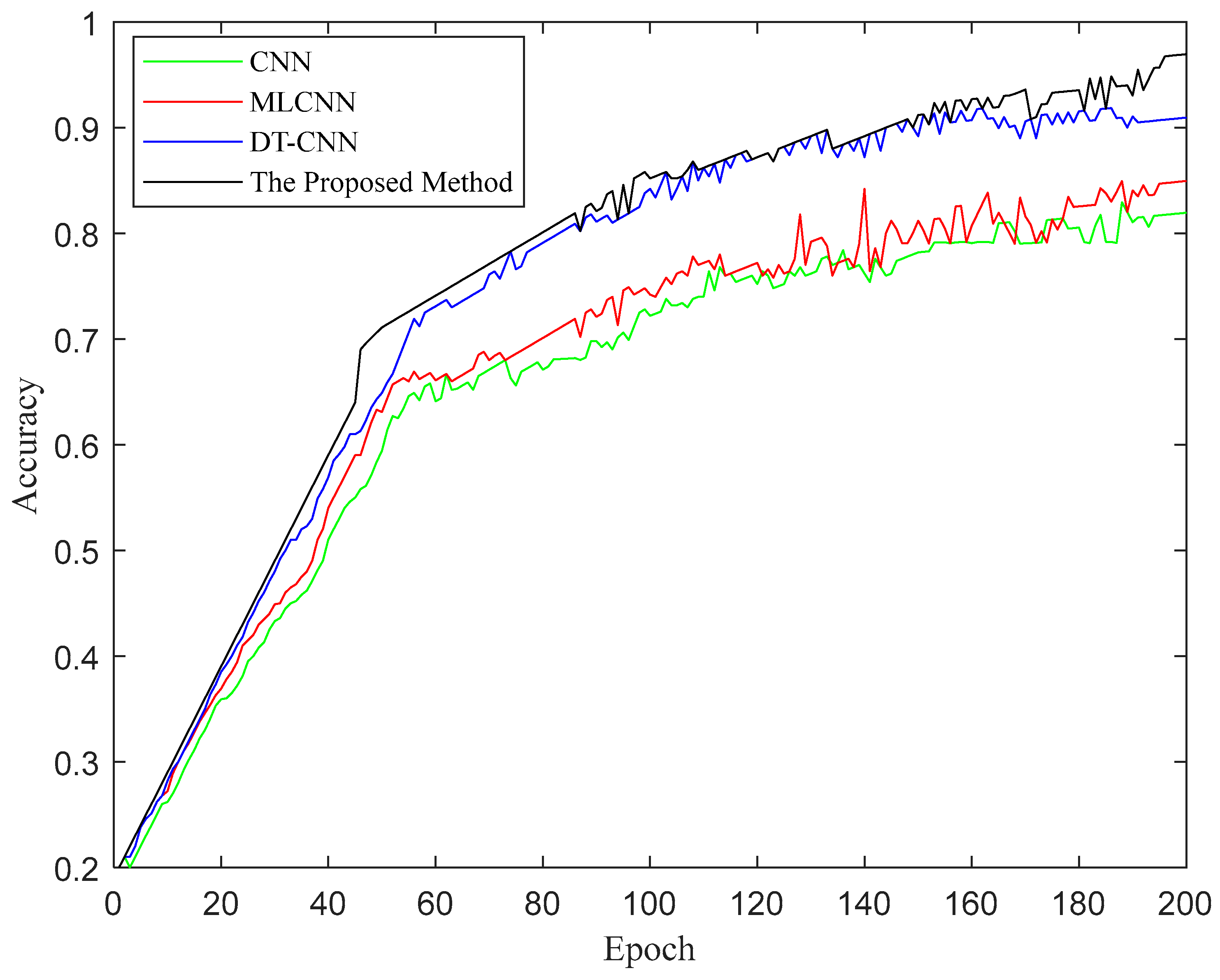
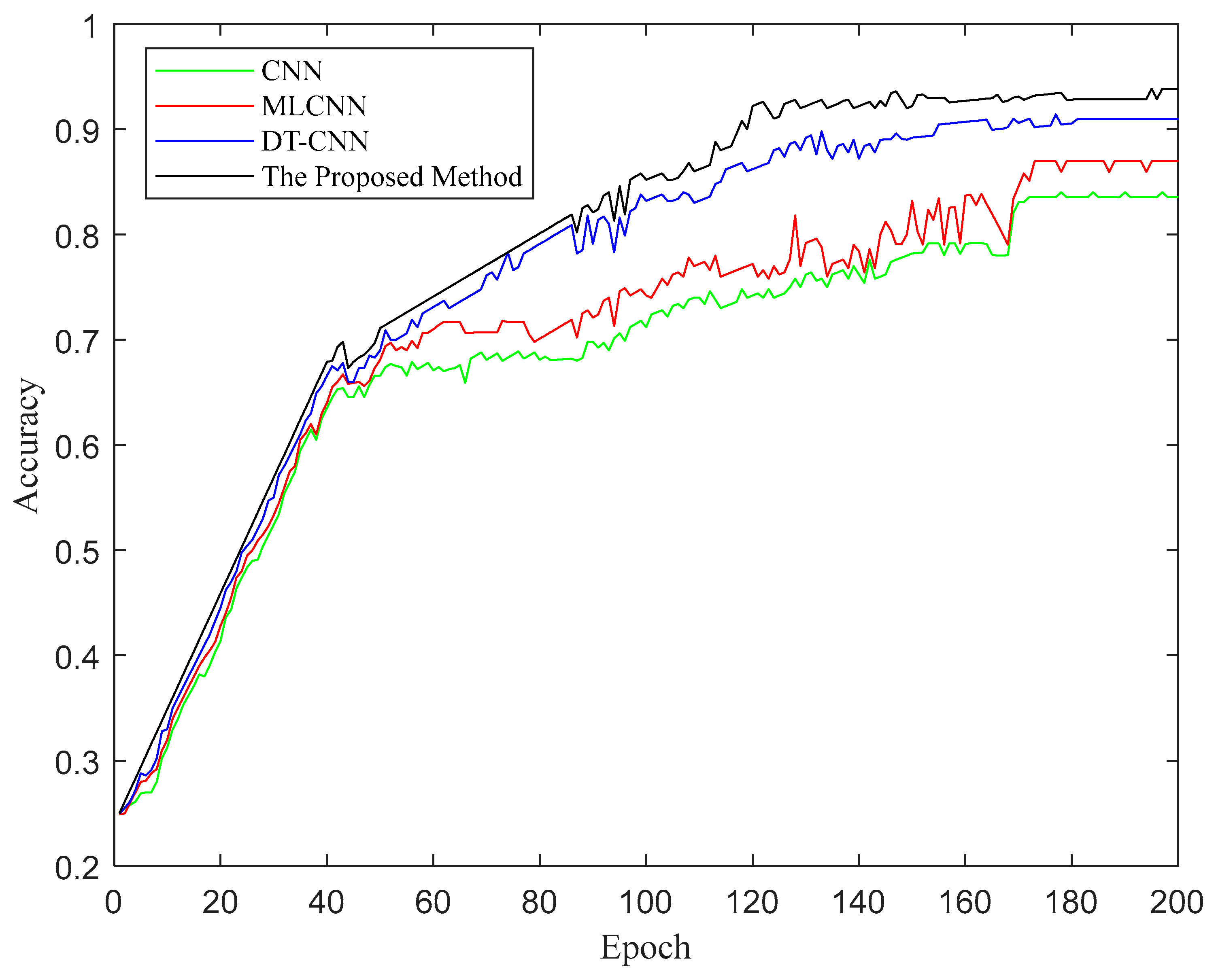
The proposed method is compared with DT-CNN, CNN, and MLCNN, and the prediction results are shown in Figure 14. The proposed method demonstrates the highest performance, showing significant efficiency in fault diagnosis. The average accuracy of the proposed method is 96.95%, which is a 15% improvement over CNN. This paper extends the proposed method by applying the trained MLCNN model to real-world bearing fault data collected from industrial robots, as shown in Figure 15. The average accuracy of the proposed method is a 14.6% improvement over CNN.

5. Discussions

As shown in Figure 14 and Figure 15, the fault diagnosis model trained with Digital Twin simulation data, when transferred to real-world data, demonstrates an improvement of approximately 15% in fault diagnosis accuracy compared to other methods, exhibiting better fault classification performance and proving its applicability for real-time bearing condition monitoring. Table 3 compares the accuracy of different existing methods, and the experimental results indicate that the proposed method significantly outperforms both the TL-ConvNext Method and the DT Drive Method, with an accuracy improvement of around 2.4%. The algorithm based on the integration of the Digital Twin model and data fusion can effectively diagnose faults in real REBs. Analysis of bearing fault diagnosis shows that the proposed method avoids lengthy fault calibration work and destructive experiments on the REB. Moreover, by utilizing models trained on high-performance servers and transferring them to real REBs, a significant reduction in model training time is achieved while maintaining good fault diagnosis performance, thereby enhancing the feasibility of predictive maintenance for REBs.

6. Conclusions

To address the issues of insufficient data, limited fault samples with imbalanced categories, and the inability to monitor real-time conditions in industrial robot REBs, a new DT-based REB fault diagnosis model is proposed. The following conclusions are drawn:
(1)
A REB fault diagnosis DT framework based on the combination of dynamic models and deep transfer learning is proposed. This transforms the traditional passive maintenance cycle into an active, preventive maintenance strategy for the entire lifecycle. Virtual entities can not only train models in virtual space to detect potential issues and fault evolution, but also interact and collaborate with physical entities for synchronous state monitoring and predictive analysis, until the end of life.
(2)
A five-degree-of-freedom dynamic twin model of the REB is constructed using MATLAB/Simulink. This model simulates and generates a large balanced dataset containing four fault states under varying operating conditions. The proposed dynamic twin model comprehensively and accurately maps the physical entity’s state behavior.
(3)
Breaking the limitations of traditional machine learning, which relies on large amounts of historical data, requires data preprocessing, and suffers from cold-start issues, a fault diagnosis algorithm based on MLCNN and transfer learning is proposed. This algorithm enables end-to-end real-time fault diagnosis of REBs from raw one-dimensional vibration signals, solving the problem of small samples in practical production and the need to retrain the model from scratch when operating conditions change.
(4)
Using the large balanced dataset simulated by DT technology, the model is pre-trained. The trained model is then transferred to actual REB operation, where it is fine-tuned and trained using real, imbalanced data to create a reliable REB fault model. This approach reduces diagnostic costs and processing time, significantly improving fault diagnosis accuracy.
The development of REB fault diagnosis technology, from traditional methods to the application of DTs and transfer learning, is an ongoing process of progress and refinement. This paper proposes a fault diagnosis DT model that integrates model knowledge of individual REB components with data-driven techniques, which can also be applied to other components, facilitating the assembly and modeling of other DTs. Future research will focus on improving the accuracy and robustness of the algorithm, reducing diagnostic costs and processing time, and further expanding its application scenarios.

Author Contributions

Conceptualization, Q.L. and M.L.; methodology, Q.L.; software, M.L.; validation, Q.L. and M.L.; formal analysis, Q.L.; investigation, M.L.; resources, Q.L.; data curation, M.L.; writing—original draft preparation, Q.L.; writing—review and editing, M.L.; visualization, Q.L.; supervision, M.L.; project administration, Q.L.; funding acquisition, Q.L. All authors have read and agreed to the published version of the manuscript.

Funding

This work was supported by the Project Supported by the Chongqing Natural Science Foundation General Project (Grant No. CSTB2025NSCQ-GPX0115), the Scientific and Technological Research Program of Chongqing Municipal Education Commission (Grant No. KJQN202503114), and the “Spark” Program Project for Teachers’ Independent Innovation at Chongqing Polytechnic University of Electronic Technology (Grant No. 25XJJSCX11).

Data Availability Statement

The raw data supporting this study can be available upon reasonable request to the authors.

Acknowledgments

The authors gratefully acknowledge Dong Zhu, Sevnce Robotics Co, Ltd., Chongqing, China for providing the local research environment.

Conflicts of Interest

The authors declare no conflict of interest.

References

  1. Sahu, D.; Dewangan, R.K.; Matharu, S.P.S. Hybrid CNN-LSTM model for fault diagnosis of rolling element bearings with operational defects. Int. J. Interact. Des. Manuf. 2025, 19, 5737–5748. [Google Scholar] [CrossRef]
  2. Li, Z.; Kristoffersen, E.; Li, J. Deep transfer learning for failure prediction across failure types. Comput. Ind. Eng. 2022, 172, 108521. [Google Scholar] [CrossRef]
  3. Keshun, Y.; Puzhou, W.; Peng, H.; Yingkui, G. A sound-vibration physical-information fusion constraint-guided deep learning method for rolling bearing fault diagnosis. Reliab. Eng. Syst. Safe. 2025, 253, 110556. [Google Scholar] [CrossRef]
  4. Lu, Q.; Li, M. Digital twin-driven remaining useful life prediction for rolling element bearing. Machines 2023, 11, 678. [Google Scholar] [CrossRef]
  5. Pandiyan, M.; Babu, T.N. Systematic review on fault diagnosis on rolling-element bearing. J. Vib. Eng. Technol. 2024, 12, 8249–8283. [Google Scholar] [CrossRef]
  6. Tang, Y.; Zhang, C.; Wu, J.; Xie, Y.; Shen, W.; Wu, J. Deep learning-based bearing fault diagnosis using a trusted multiscale quadratic attention-embedded convolutional neural network. IEEE Trans. Instrum. Meas. 2024, 73, 3513215. [Google Scholar] [CrossRef]
  7. Habbouche, H.; Amirat, Y.; Benkedjouh, T.; Benbouzid, M. Digital twin-based gearbox fault diagnosis using variational mode decomposition and dynamic vibration modeling. Measurement 2025, 246, 116669. [Google Scholar] [CrossRef]
  8. Misbah, I.; Lee, C.K.; Keung, K.L. Fault diagnosis in rotating machines based on transfer learning: Literature review. Knowl.-Based Syst. 2024, 283, 111158. [Google Scholar] [CrossRef]
  9. Yang, B.; Lei, Y.; Li, X.; Li, N. Targeted transfer learning through distribution barycenter medium for intelligent fault diagnosis of machines with data decentralization. Expert Syst. Appl. 2024, 244, 122997. [Google Scholar] [CrossRef]
  10. Zhao, L.; Xie, T.; Wei, Y.; Liu, Y.; Qin, Y. Overview of digital twin-driven rotating machinery fault diagnosis: Status and trends. Meas. Sci. Technol. 2025, 36, 052001. [Google Scholar] [CrossRef]
  11. Wang, D.; Chen, C. Multilevel feature encoder for transfer learning-based fault detection on acoustic signal. Inform. Fusion 2025, 121, 103128. [Google Scholar] [CrossRef]
  12. Chen, X.; Yang, R.; Xue, Y.; Huang, M.; Ferrero, R.; Wang, Z. Deep transfer learning for bearing fault diagnosis: Asystematic review since 2016. IEEE Trans. Instrum. Meas. 2023, 72, 3508221. [Google Scholar] [CrossRef]
  13. Yan, P.; Abdulkadir, A.; Luley, P.P.; Rosenthal, M.; Schatte, G.A.; Grewe, B.F.; Stadelmann, T. A comprehensive survey of deep transfer learning for anomaly detection in industrial time series: Methods, applications, and directions. IEEE Access 2024, 12, 3768–3789. [Google Scholar] [CrossRef]
  14. Xiang, S.; Li, P.; Luo, J.; Qin, Y. Micro transfer learning mechanism for cross-domain equipment RULprediction. IEEE Trans. Autom. Sci. Eng. 2025, 22, 1460–1470. [Google Scholar] [CrossRef]
  15. Zheng, L.; Zhu, Y.; Zhou, Y. Meta-transfer learning-based method for multi-fault analysis and assessment in power system. Appl. Intell. 2024, 54, 12112–12127. [Google Scholar] [CrossRef]
  16. Zheng, B.; Huang, J.; Ma, X.; Zhang, X.; Zhang, Q. An unsupervised transfer learning method based on SOCNN and FBNN and its application on bearing fault diagnosis. Mech. Syst. Signal Process. 2024, 208, 111047. [Google Scholar] [CrossRef]
  17. Pathak, K.A.; Kafle, P.; Vikram, A. Deep learning-based defect detection in film-coated tablets using a convolutional neural network. Int. J. Pharm. 2025, 671, 125220. [Google Scholar] [CrossRef]
  18. Azad, M.M.; Shah, A.U.R.; Prabhakar, M.N.; Kim, H.S. Deep learning-based autonomous morphological fracture analysis of fiber-reinforced composites. Eng. Fail. Anal. 2025, 170, 109292. [Google Scholar] [CrossRef]
  19. He, D.; Zhao, J.; Jin, Z.; Huang, C.; Zhang, F.; Wu, J. Prediction of bearing remaining useful life based on a two-stage updated digital twin. Adv. Eng. Inform. 2025, 65, 103123. [Google Scholar] [CrossRef]
  20. Sohel, R. AI-driven fault detection and predictive maintenance in electrical power systems: A systematic review of data-driven approaches, digital twins, and self-healing grids. Am. J. Adv. Technol. Eng. Solut. 2025, 1, 258–289. [Google Scholar]
  21. Mikołajewska, E.; Mikołajewski, D.; Mikołajczyk, T.; Paczkowski, T. Generative AI in AI-based digital twins for fault diagnosis for predictive maintenance in Industry 4.0/5.0. Appl. Sci. 2025, 15, 3166. [Google Scholar] [CrossRef]
  22. Sun, Z.; Wang, Y.; Chen, Z. Fault diagnosis method for proton exchange membrane fuel cell system based on digital twin and unsupervised domain adaptive learning. Int. J. Hydrogen Energy 2024, 50, 1207–1219. [Google Scholar] [CrossRef]
  23. Gong, S.; Li, S.; Zhang, Y.; Zhou, L.; Xia, M. Digital twin-assisted intelligent fault diagnosis for bearings. Meas. Sci. Technol. 2024, 35, 106128. [Google Scholar] [CrossRef]
  24. Ye, W.; Liu, X.; Zhao, X.; Fu, H.; Cai, Y.; Li, H. A data-driven digital twin architecture for failure prediction of customized automatic transverse robot. IEEE Access 2024, 12, 59222–59235. [Google Scholar] [CrossRef]
  25. Yin, Y.; Chen, H.; Meng, X.; Xie, H. Digital twin-driven identification of fault situation in distribution networks connected to distributed wind power. Int. J. Elec. Power Energ. Syst. 2024, 155, 109415. [Google Scholar] [CrossRef]
  26. Xue, R.; Zhang, P.; Huang, Z.; Wang, J. Digital twin-driven fault diagnosis for CNCmachine tool. Int. J. Adv. Manuf. Technol. 2024, 131, 5457–5470. [Google Scholar] [CrossRef]
  27. Grieves, M. Intelligent digital twins and the development and management of complex systems. Digit. Twin 2024, 1, 8. [Google Scholar] [CrossRef]
  28. Sawalhi, N.; Randall, R.B. Simulating gear and bearing interactions in the presence of faults: Part I. The combined gear bearing dynamic model and the simulation of localised bearing faults. Mech. Syst. Signal Pract. 2008, 22, 1924–1951. [Google Scholar] [CrossRef]
  29. Dong, Y.; Li, Y.; Zheng, H.; Wang, R.; Xu, M. A new dynamic model and transfer learning based intelligent fault diagnosis framework for rolling element bearings race faults: Solving the small sample problem. ISA Trans. 2022, 121, 327–348. [Google Scholar] [CrossRef] [PubMed]
  30. Cheng, J.; Huang, K.; Zheng, Z. Towards better forecasting by fusing near and distant future visions. Proc. AAAI Conf. Artif. Intell. 2020, 34, 3593–3600. [Google Scholar] [CrossRef]
  31. Zhang, C.; Qin, F.; Zhao, W.; Li, J.; Liu, T. Research on rolling bearing fault diagnosis based on digital twin data and improved ConvNext. Sensors 2023, 23, 5334. [Google Scholar] [CrossRef] [PubMed]
  32. Qin, Y.; Liu, H.; Mao, Y. Faulty rolling bearing digital twin model and its application in fault diagnosis with imbalanced samples. Adv. Eng. Inform. 2024, 61, 102513. [Google Scholar] [CrossRef]
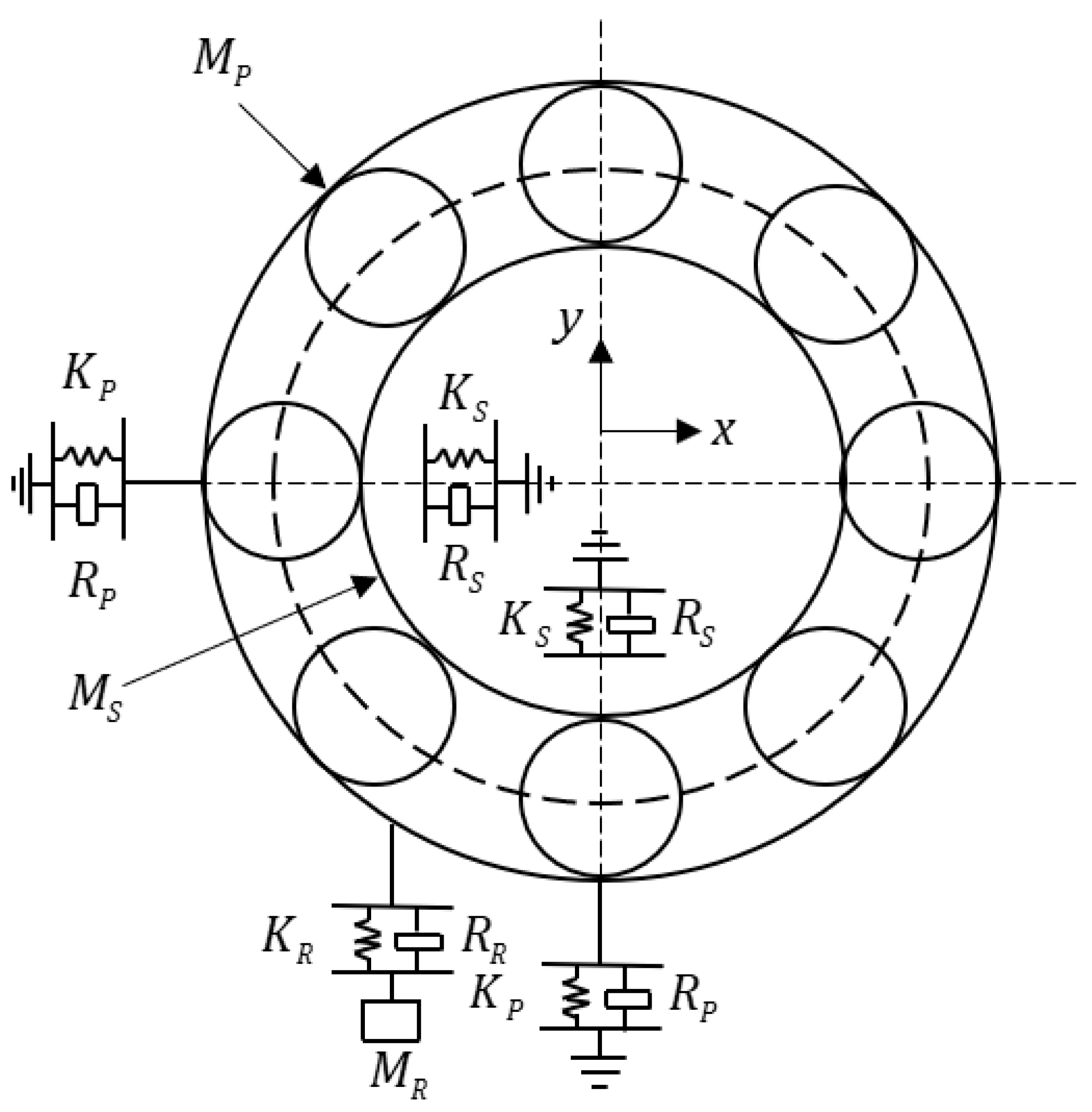
Figure 1. Five-degree-of-freedom dynamic model of the REB.
Applsci 15 12509 g001
Figure 2. Scratches on inner or outer raceway.
Applsci 15 12509 g002
Figure 3. Rolling element fault illustration.
Applsci 15 12509 g003
Figure 4. Intelligent prediction model structure for deep transfer learning assisted by DTs.
Applsci 15 12509 g004
Figure 5. Intelligent prediction process of DT-assisted deep transfer learning.
Applsci 15 12509 g005
Figure 6. The experimental platform.
Applsci 15 12509 g006
Figure 7. The DT model of the REB.
Applsci 15 12509 g007
Figure 8. Simulated vibration signal of the REB in the DT model.
Applsci 15 12509 g008
Figure 9. Simulated vibration signal of the REB in the DT model after denoising.
Applsci 15 12509 g009
Figure 10. Training results of the DT model simulated vibration signal.
Applsci 15 12509 g010
Figure 11. The actual fault data.
Applsci 15 12509 g011
Figure 12. The actual fault data after denoising.
Applsci 15 12509 g012
Figure 13. The prediction results of REB faults based on deep transfer learning.
Applsci 15 12509 g013
Figure 14. The prediction results of REB faults based on different methods.
Applsci 15 12509 g014
Figure 15. The prediction results of industrial robot REB faults based on different methods.
Applsci 15 12509 g015
Table 1. The fault data of the REB.
Fault TypeSpeed (rpm/min)
Normal REB 400500600700
Inner Ring Fault of REB400500600700
Outer Ring Fault of REB 400500600700
Rolling Element Fault of REB400500600700
Table 2. The comparison of the DT data and actual data.
DataPeak ValueRMS ValueSkewnessFrequency Domain Feature
Actual Data6 g10.3 g542120 Hz
DT Data6.3 g10.4 g562122 Hz
Error5%0.97%7.54%1.67%
Table 3. The accuracy comparison of various methods.
MethodAccuracy
TL-ConvNext Method [31]94.6%
DT Drive Method [32]95.6%
The proposed method96.95%
Disclaimer/Publisher’s Note: The statements, opinions and data contained in all publications are solely those of the individual author(s) and contributor(s) and not of MDPI and/or the editor(s). MDPI and/or the editor(s) disclaim responsibility for any injury to people or property resulting from any ideas, methods, instructions or products referred to in the content.