Gaze Point Estimation via Joint Learning of Facial Features and Screen Projection

Abstract

In recent years, gaze estimation has received a lot of interest in areas including human–computer interface, virtual reality, and user engagement analysis. Despite significant advances in convolutional neural network (CNN) techniques, directly and effectively predicting the point of gaze (PoG) in unconstrained situations remains a difficult task. This study proposes a gaze point estimation network (L1fcs-Net) that combines facial features with positional features derived from a two-dimensional array obtained by projecting the face relative to the screen. Our approach incorporates a Face-grid branch to enhance the network’s ability to extract features such as the relative position and distance of the face to the screen. Additionally, independent fully connected layers regress x and y coordinates separately, enabling the model to better capture gaze movement characteristics in both horizontal and vertical directions. Furthermore, we employ a multi-loss approach, balancing classification and regression losses to reduce gaze point prediction errors and improve overall gaze performance. To evaluate our model, we conducted experiments on the MPIIFaceGaz dataset, which was collected under unconstrained settings. The proposed model achieves state-of-the-art performance on this dataset with a gaze point prediction error of 2.05 cm, demonstrating its superior capability in gaze estimation.

1. Introduction

Humans obtain 80–90% of external information through their eyes. Visual perception of information can be captured via eye tracking [1]. Point of Gaze (PoG) estimation, as one of the core tasks in eye tracking, aims to predict the user’s gaze location from facial or eye images. PoG estimation not only facilitates more natural and efficient interaction methods [2,3] but also plays a vital role across diverse fields, including healthcare [4,5], psychological research [6,7], virtual reality [8], and assistive technology [9,10]. Consequently, researchers have developed various techniques and methods to accurately estimate the PoG. These approaches fall into two categories: model-based methods and appearance-based methods. Model-based methods typically require specialized hardware, limiting their use in unconstrained environments. Appearance-based methods directly regress human gaze from images captured by inexpensive off-the-shelf cameras, enabling easy deployment across diverse locations with minimal setup constraints.

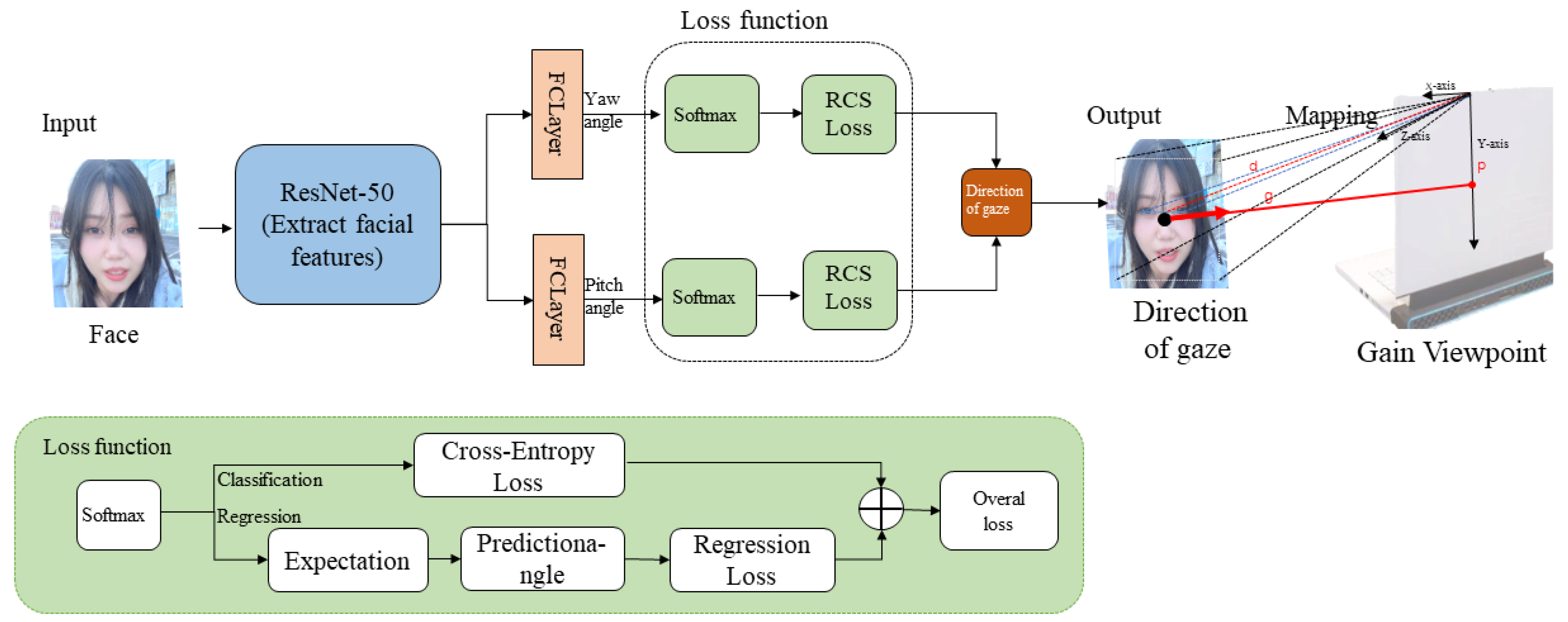
Recently, methods based on convolutional neural networks (CNNs) have become the most widely used eye-tracking estimation techniques. Table 1 summarizes the usage and error metrics (geometric distance between actual and predicted pixel coordinates) for common gaze point estimation models. According to existing literature, two common gaze point estimation methods exist. The first method structure is shown in Figure 1. Most related work focuses on developing novel CNN architectures to extract gaze features and output gaze direction [11,12,13]. For example, Abdelrahman et al. [14] proposed a fine-grained gaze estimation method that can directly predict pitch and yaw angles from images.

This method estimates the gaze point on a two-dimensional plane by calculating the intersection point between the extended line of the gaze direction and the gaze plane [15]. However, methods using gaze direction to estimate the fixation point accumulate errors from both the detection phase and the gaze line estimation phase. These errors stem not only from deviations in the gaze direction estimation algorithm but also from inaccuracies in calculating the starting point of the gaze direction (the center point of the outer canthi of both eyes). This starting point is primarily derived from the interocular distance between the outer canthi. Consequently, the detection accuracy of the outer canthus keypoints and the interocular distance set under reference conditions both introduce computational errors. Moreover, implementing gaze point estimation via gaze direction is relatively complex. When the acquisition device’s position or orientation relative to the gaze plane changes, recalibration of camera parameters is required to obtain the transformation matrix between the altered camera coordinate system and the world coordinate system. During facial yaw movements, detection errors of the outer canthi increase, leading to larger gaze point estimation errors.

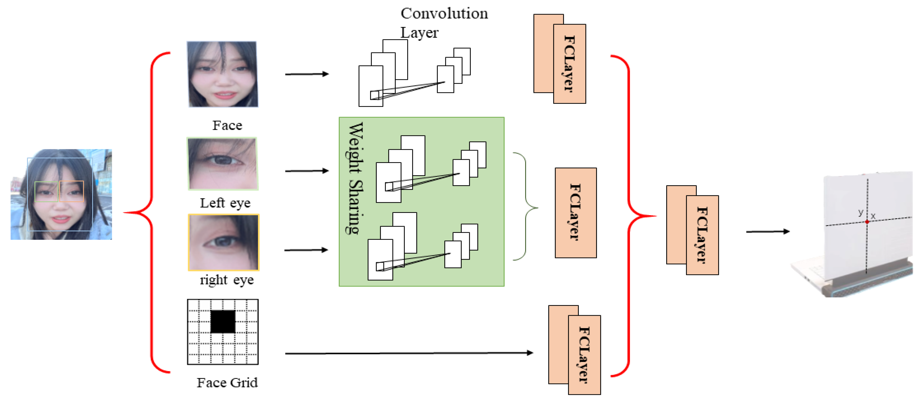
The second method, structured as shown in Figure 2, enables gaze point estimation by training a deep neural network to learn the mapping relationship between input images and the position of the gaze point on a 2D plane [16]. Krafka et al. [17] proposed the iTracker network, which uses facial images, left/right eye images, facial grids, and binocular images as input signals for the gaze estimation algorithm to directly obtain a 2D gaze point. However, it lacks the precision required for fine-grained gaze point localization on the screen.

Kim et al. [18] further investigated classification-regression functions to enhance the precision of fixation points, but the issue of complex network structures remains an ongoing area of research.

Therefore, a review of existing gaze estimation literature reveals two key limitations: (1) End-to-end methods that directly output gaze points require multiple input streams, resulting in high computational complexity and insufficient accuracy; (2) Methods deriving gaze points from gaze direction necessitate manual setting of the distance between the face and screen, introducing errors, and require additional modeling to map gaze points to the screen, thereby increasing computational complexity.

Table 1. Gaze Point Estimation Model Methods and Experimental Error/cm.

Model	Primary Methods	Parameters (M)	Inference Time (ms)	FPS	Absolute Error/cm
iTracker	Feature Fusion Across Multiple Facial Datasets	6.78	None	10–15	7.25
AFF-Net [19]	Adaptive Fusion of Left and Right Eye Features Based on Similarity	None	None	None	4.21
CA-Net [20]	Add the base direction and residual to obtain the final gaze direction.	None	None	None	4.50
GazeNets [21]	Integrating ocular image features and head posture information	None	138	None	6.42
FullFace [22]	Full-face appearance-based gaze estimation using deep convolutional networks	196.6	50	None	5.54
Ours	The fusion face is gazing at the screen projection position.	28.16	12	100	2.05

Table 1. Gaze Point Estimation Model Methods and Experimental Error/cm.

Model	Primary Methods	Parameters (M)	Inference Time (ms)	FPS	Absolute Error/cm
iTracker	Feature Fusion Across Multiple Facial Datasets	6.78	None	10–15	7.25
AFF-Net [19]	Adaptive Fusion of Left and Right Eye Features Based on Similarity	None	None	None	4.21
CA-Net [20]	Add the base direction and residual to obtain the final gaze direction.	None	None	None	4.50
GazeNets [21]	Integrating ocular image features and head posture information	None	138	None	6.42
FullFace [22]	Full-face appearance-based gaze estimation using deep convolutional networks	196.6	50	None	5.54
Ours	The fusion face is gazing at the screen projection position.	28.16	12	100	2.05

As shown in Table 1, existing gaze point estimation methods struggle to achieve a balance between accuracy, speed, and parameter efficiency. Specifically: (1) High-parameter methods like FullFace-25 employ a deep convolutional network with 196.6 million parameters, yet suffer from redundant parameters despite achieving only 5.54 cm accuracy and 50 ms inference time; (2) Multimodal fusion methods like GazeNet-24 integrate eye images and head pose information, but its 138 ms inference latency renders it unsuitable for real-time interactive scenarios; (3) Lightweight methods such as iTracker-18 feature only 6.78 M parameters and relatively fast speed (10–15 FPS), yet its 7.25 cm error falls far short of high-precision requirements; (4) Even the most accurate methods, AFF-Net-40 (4.21 cm) and CA-Net-39 (4.50 cm), lack reported inference times and parameter counts, casting doubt on their engineering practicality.

To address these issues, this paper proposes a method that uses facial images containing gaze information and a facial grid representing the face’s relative position on the screen as input, simplifying the complex structure required to obtain the gaze point. This approach employs independent fully connected layers to regress x and y coordinates separately, enabling more precise extraction of relevant features in both directions. We propose a classification-based eye-point localization method that divides the screen into 69 × 39 regions for coarse eye-point category estimation, thereby reducing computational cost. Two independent loss functions (each containing classification and regression components) predict eye-point positions, effectively enhancing model stability.

2. Related Work

According to the literature, appearance-based gaze estimation algorithms can be categorized into traditional methods and appearance-based methods.

2.1. Gaze Estimation Methods for Traditional Function Mappings

Traditional gaze estimation methods employ regression functions to create specific mappings to human gaze, such as adaptive linear regression and Gaussian process regression [23,24,25]. These methods demonstrate reasonable accuracy in constrained settings (e.g., subject-specific and fixed head posture and lighting); however, their performance degrades significantly when tested in unconstrained settings.

2.2. Deep Learning-Based Gaze Estimation Methods

Deep learning-based methods can simulate highly nonlinear mapping functions between images and gaze point locations. Zhang et al. first proposed a simple CNN-based architecture using monocular images to predict gaze, while subsequent studies demonstrated that combining features from both eyes improves the accuracy of gaze estimation. Fischer et al. employed two VGG-16 networks to extract individual features from both eye images, then concatenated these features for regression analysis. However, simply combining binocular features into a new feature vector yielded only marginal improvements in gaze estimation accuracy. Wang et al. [26] proposed an adversarial learning method to extract invariant features from eye images. This approach feeds features into an additional classifier and designs an adversarial loss function to handle variations in appearance across subjects. Kim et al. [27] employed GANs to convert low-light images to high-light images; Rangesh et al. [28] used GANs to remove eyeglasses. Beyond supervised feature extraction, unlabeled eye images can also be utilized for feature extraction. Yu et al. [29] employed unsupervised learning [30] using unlabeled eye images, inputting the differences between both eyes into the network. Subsequent research revealed that facial images contain head pose information, aiding gaze estimation. Several studies directly utilized full-face images as input, achieving significant performance improvements over methods relying solely on eye images.

Recently, Abdelrahman et al. proposed a fine-grained gaze estimation method. This approach directly predicts pitch and yaw angles from images. It employs a multi-loss network incorporating angle classification loss and regression loss. The classification loss categorizes gaze angles into distinct classes, while the regression loss predicts pitch and yaw angles. The classification loss categorizes angles, whereas the regression loss predicts angular deviations from the target. By weighting the classification and regression losses, the network learns to predict precise gaze angles. However, the coarse classification leads to quantization loss. Hu et al. [31] proposed the HG-Net coarse-fine hybrid classification framework, which not only enables finer angle classification but also improves prediction performance. Methods including [32,33,34] have advanced the field of gaze estimation, but they primarily focus on 3D gaze direction estimation. Obtaining specific 2D gaze point coordinates requires substantial computational resources.

Krafka et al. proposed the iTracker network, which combines inputs from left and right eye images, facial images, and facial meshes containing positional information to directly obtain gaze point locations. However, it lacks the precision required for fine gaze point localization on screens. Building upon this, Kim S. et al. investigated classification-regression functions to enhance gaze point accuracy, though the issue of complex network structures remains an ongoing research topic.

Therefore, this paper proposes a gaze point estimation network (L1fcs-Net) that integrates the face with the projected gaze position on the screen, aiming to improve gaze point prediction accuracy while conserving computational resources and simplifying the network structure. This network utilizes both the facial image and a facial mesh containing relative position information as inputs. Independent fully connected layers regress each coordinate separately, enabling the model to better capture gaze movement features in both horizontal and vertical directions. A classifier module predicts the horizontal and vertical positions of the gaze point, respectively, while a loss function achieves a coarse estimate of the gaze point. Simultaneously, the predicted classification is refined through regression functions to achieve precise gaze point estimation. This classification-and-regression-weighted approach mitigates large-scale errors inherent in direct regression models, enhancing robustness.

3. L1fcs-Net Network

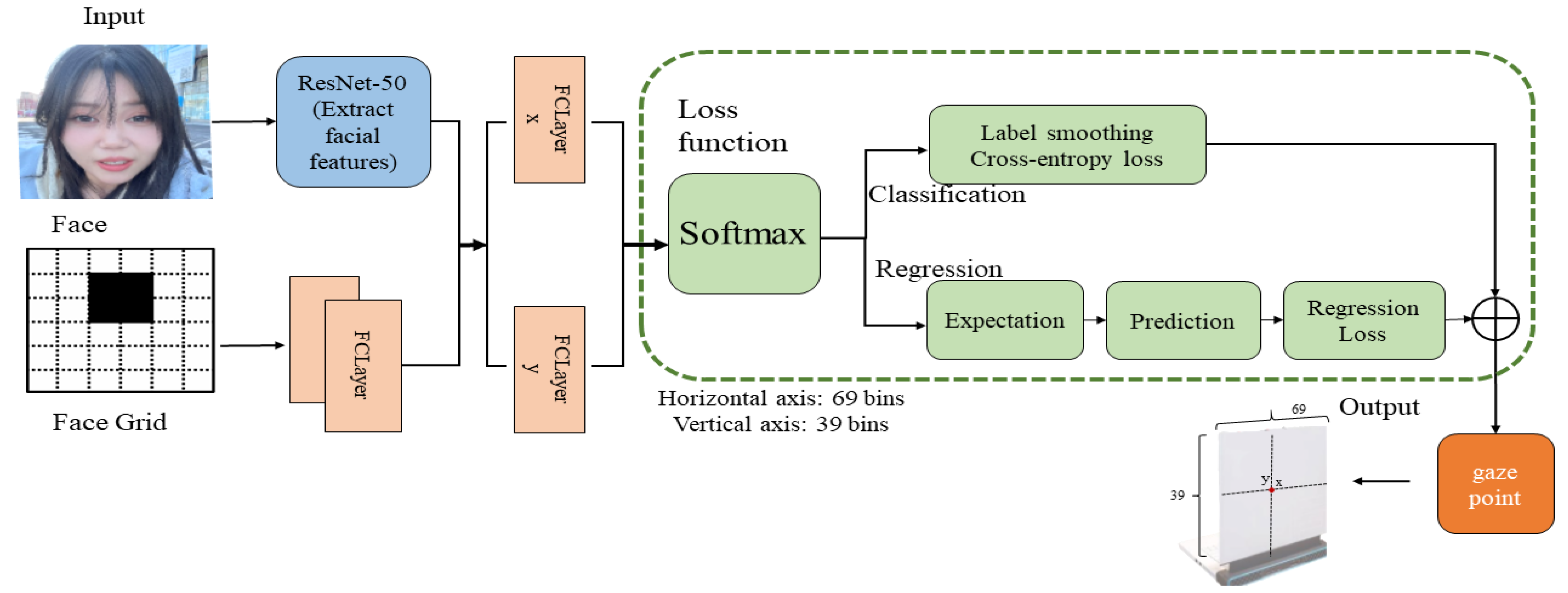
Figure 3 depicts the L2cs-2D-Net model architecture, a novel network model for 2D gaze point estimation. The facial image branch of this network employs ResNet-50 [35,36] as its backbone for extracting gaze features. The face grid branch utilizes two fully connected layers to extract the relative position of the face on the screen. By integrating coordinate information from both branches and employing two fully connected layers to independently regress and predict each gaze coordinate (x, y), the model directly obtains the x and y coordinates of the gaze point on the screen. A multi-loss combination function is employed for backpropagation and network weight adjustment, enhancing both the generalization capability and prediction accuracy of this network architecture.

3.1. Model

The proposed L1fcs-Net model takes face images (224 × 224) and face meshes (25 × 25) as inputs. The face image branch employs ResNet-50 to extract 2048-dimensional features containing gaze information, while the face mesh branch utilizes two fully connected layers to extract 625-dimensional relative position features. These features are concatenated into a 2673-dimensional representation, which is then processed by two independent fully connected branches to predict x and y coordinates.

To achieve multi-task learning, the gaze pixel coordinates are discretized into classification units: at 1920 × 1080 resolution, the horizontal direction is divided into 69 intervals and the vertical direction into 39 intervals. The model achieves collaborative learning by jointly optimizing classification and regression losses: logit values from the fully connected layer undergo softmax transformation to generate classification probability distributions, while smooth L1 loss handles the regression task. This multi-objective loss strategy integrates cross-entropy classification loss with smooth L1 regression loss, constructing an end-to-end framework that significantly enhances model robustness and training stability.

3.2. Classification and Regression Fusion Output

To obtain the final gaze point coordinates, L1fcs-Net employs a coarse-to-fine fusion strategy. The classification branch, responsible for coarse localization, outputs logit values for the x and y dimensions, which are then converted into probability distributions via softmax. The grid index corresponding to the maximum probability is selected as the coarse gaze point location:

$$\begin{gathered} bi{n}_x=-\arg \max \left(soft\max \left(X_{cls}\right)\right), \\ bi{n}_y=-\arg \max \left(soft\max \left(y_{cls}\right)\right). \end{gathered}$$

(1)

where $bi{n}_x\in \left[0, 68\right]$ and $bi{n}_y\in \left[0, 38\right]$ denotes the predicted x-coordinate grid index, and the predicted y-coordinate grid index. This classification step reduces the search space from 2,073,600 pixels (1920 × 1080) to 2691 grid cells (69 × 39), lowering computational complexity by approximately 770 times.

The discrete grid indices are then converted to continuous coordinates within the normalized space [−1, 1]:

$$\begin{gathered} cente{r}_x=-1+2(bi{n}_x+0.5)/69, \\ cente{r}_y=-1+2(bi{n}_y+0.5)/39. \end{gathered}$$

(2)

Adding 0.5 aligns coordinates to grid midpoints rather than boundaries, providing baseline estimates for subsequent optimization. The regression branch outputs continuous offset values constrained within the range [−0.9, 0.9]. The Tanh activation function ensures adjustments remain confined to a single grid cell.

Finally, the normalized coordinates are mapped to screen pixel coordinates. This fusion mechanism fully leverages the complementary strengths of classification and regression: the classification branch achieves stable global localization through discrete grid predictions, while the regression branch attains sub-pixel accuracy via continuous offset adjustments. This coarse-to-fine strategy effectively balances localization precision and robustness, enabling the model to maintain stable performance across diverse scenarios. Compared to pure classification (error of 2.19 cm) or pure regression (error of 2.23 cm), the proposed fusion strategy achieves an accuracy of 2.05 cm (shown in

Table 2. Parameter Distribution.

Structure	Parameters (M)	FLOPs (G)
ResNet-50	25.6	4.1
Face grid branch	1.6	0.08
Regression branch	2.4	0.14
Classification branch	3.8	0.14

)—representing improvements of 6.39% and 9.1%, respectively—validating the effectiveness of the two-stage fusion approach.

3.3. Loss Functions

To enhance model performance, this paper adopts a multi-task loss function strategy, imposing independent loss constraints on the horizontal and vertical coordinates, respectively, to decouple the mutual interference between the two dimensions. Based on reference [15], this paper applies cross-entropy loss for the classification task and adopts Smooth L1 Loss instead of mean squared error (MSE) for the regression task, effectively mitigating gradient oscillations caused by samples with large errors during training, thereby significantly improving the stability of model training. The overall loss function for each coordinate axis is defined as in Equation (3):

$$\begin{gathered} L_x=L_{x\_cls}+\lambda L_{x\_reg}, \\ {L}_{\mathrm{y}}=L_{\mathrm{y}\_cls}+\lambda L_{\mathrm{y}\_reg}, \\ {L}_{total}=L_x+L_x. \end{gathered}$$

(3)

Here, λ is a hyperparameter for the regression loss weight (set to λ = 1 in the experiments), $L_{\mathrm{y}\_cls}$ representing the classification loss for x and y coordinates, $L_{x\_reg}$ and corresponding to their respective regression losses.

In addition, this work discretizes continuous gaze coordinates into a classification task: the x coordinates are divided into $N_{\mathrm{x}}=69$ several intervals, and the y coordinates are also divided into $N_y=39$ several intervals. The classification loss is calculated using label-smoothed cross-entropy, as shown in Equation (4):

$$\begin{gathered} L_{x\_cls}=-{\displaystyle \sum _{j=1}^{N_x}{q}_j\log \left(p_j^x\right)}, \\ {L}_{y\_cls}=-{\displaystyle \sum _{j=1}^{N_y}{q}_j\log \left(p_j^y\right)}. \end{gathered}$$

(4)

Here, $p_j^y$ represents the probability of the $j$-th interval output by softmax, as indicated in Formula (5):

$$p_j^x={\displaystyle \frac{\exp \left(z_j^x\right)}{{\displaystyle {\sum }_{k-1}^{N_x}\exp \left(z_j^x\right)}}}$$

(5)

Here, $z_j^x$ represents the th logit value output by the fully connected layer. The label smoothing strategy converts hard labels into a soft label distribution as shown in Equation (6):

$$q_{ij}^x=y_{ij}^x\left(1-\epsilon \right)+{\displaystyle \frac{\epsilon }{B_x}}$$

(6)

Here, $q_{ij}^x$ represents the interval index to which the true x-coordinate of sample i belongs, and $\epsilon$ is the smoothing factor (set to 0.1 in this paper). Label smoothing assigns small probability values ($\epsilon /B_x$) to non-true classes, effectively preventing the model from being overconfident in a single class and reducing the risk of overfitting. In particular, when gaze point data may contain annotation noise or uneven distribution, label smoothing can significantly enhance the model’s robustness and generalization ability. In addition, the smoothed softmax output stabilizes the expected coordinates predicted by the classification branch, indirectly reducing the consistency loss with the regression branch and promoting the collaborative optimization of both branches.

The regression branch in this study uses the Smooth L1 loss function, which is used for fine localization within the coarse intervals determined by classification, as shown in Equation (7):

$$\begin{gathered} L_{x\_reg}={\displaystyle \frac{1}{N}}{\displaystyle \sum _{i=1}^{N}SmoothL1\left(x_i^{gt}-\stackrel{\wedge }{x_i^{reg}}\right)}, \\ {L}_{y\_reg}={\displaystyle \frac{1}{N}}{\displaystyle \sum _{i=1}^{N}SmoothL1\left(y_i^{gt}-\stackrel{\wedge }{y_i^{reg}}\right)}, \\ SmoothL1(x)=\left\{\begin{array}{l}0.5x^2,if\left|x\right|<\delta \\ \left|x\right|-0.5\delta ,otherwise\end{array}\right.. \end{gathered}$$

(7)

Among them, $\delta =x_i^{gt}-\stackrel{\wedge }{x_i^{reg}}$ represents the prediction error, $x_i^{gt}$ and $y_i^{gt}$ are the true coordinates, $\stackrel{\wedge }{x_i^{reg}}$ and $\stackrel{\wedge }{y_i^{reg}}$ these are the continuous coordinate values predicted by the regression branch. The Smooth L1 loss combines the advantages of being sensitive to small errors and robust to large errors. It uses a quadratic function to smooth the gradient when the error is small and a linear function to avoid gradient explosion when the error is large, thereby improving training stability.

The final loss is obtained by weighted fusion of the classification and regression losses. During training, the classification branch first locates the gaze points in coarse intervals, providing global positioning information, while the regression branch subsequently performs sub-pixel fine adjustments within that interval. The two branches complement each other through shared feature representations and joint optimization: the classification loss guides the model to learn discriminative regional features, and the regression loss enhances local precision. This coarse-to-fine strategy effectively balances localization accuracy and robustness, enabling the model to maintain stable predictive performance in complex scenarios.

4. Experiments

4.1. Datasets

With the growing demand for deep learning-based methods to enhance gaze estimation accuracy, large-scale datasets have emerged. These datasets span diverse environments, ranging from controlled laboratory settings to unconstrained outdoor scenarios. In this paper, the MPII-FaceGaze dataset [37] is employed to train the model, aiming to improve the versatility of the network architecture in terms of precision.

4.1.1. MPII-FaceGaze Dataset Preprocessing

This dataset is one of the most widely used datasets for appearance-based gaze estimation algorithms. Data was collected in uncontrolled environments, featuring images under varying backgrounds and lighting conditions, along with natural head movements during data acquisition. Each of the 15 participants has an independent folder containing daily facial images, totaling 213,659 images. As shown in Figure 4: 100% screen view coverage and 78.24% head pose coverage. However, when eye tracking was interrupted due to blinking, prolonged eye closure, head pose exceeding tracking range, temporary failure of facial feature recognition, or occlusion of the face/eyes by hands, hair, or objects, the annotation system recorded default values (0,0) as placeholders. This occurred in 2564 samples, accounting for 12% of the dataset.

Therefore, all (0, 0) samples were removed during experimentation, and the dataset was reconstructed to achieve robust gaze estimation capabilities across diverse environments. Through five-fold cross-validation, the dataset was divided into five subsets. In each training iteration, one subset is selected as the test set, while the remaining four serve as the training set. The model is trained on the training set and evaluated on the validation set. This process is repeated five times. Averaging the results mitigates the inherent randomness of single-round splits, reduces overfitting risks, and enables more reliable model performance assessment.

4.1.2. Label Classification Preprocessing

The gaze point estimation method in this paper directly estimates the landing point of the user’s gaze on the screen. However, since the human gaze perceives not just a single point but an entire area encompassing the target and its surroundings at a certain distance, the gaze point estimation task inherently involves an error. Observations indicate that at a typical viewing distance of approximately 50 cm from the screen, the human eye can simultaneously perceive 3 to 5 characters (spaced roughly 2 cm apart horizontally) within the same line of sight. Considering the typical size of standard software interface elements, the corresponding button area occupies a square region with a side length of approximately 0.5 cm. Therefore, in this study’s two-dimensional gaze point estimation task, the target screen is divided into intervals of 5 mm in both the horizontal and vertical directions. A 15.6-inch laptop screen is horizontally divided into 69 intervals and vertically into 39 regions. Since the dataset labels specify gaze point positions using pixel coordinates, the labels require preprocessing before application in 2D gaze point estimation. Based on the 1920 × 1080 resolution of the personal laptop used in experiments, the screen is divided into 69 intervals along the horizontal pixel dimension and 39 intervals along the vertical pixel dimension. Using the target screen size and resolution information provided in the dataset, the annotated actual gaze points were converted from pixel coordinates to Euclidean coordinates. The horizontal and vertical categories were numbered starting from 1.

4.1.3. Face Grid Preprocessing

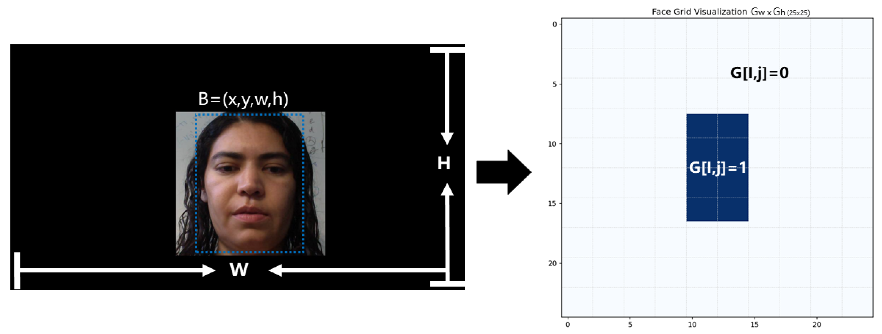
The facial mesh generation is illustrated in Figure 5. This mesh represents a two-dimensional array of the face image projected relative to the screen, providing positional and distance features of the face relative to the screen. This method utilizes the dlib facial landmark detection algorithm to detect the facial region within the input image and obtain its bounding box coordinates ($x,y,h,w$).

Original image dimensions: $W\times H$; Experimental target grid dimensions: $G_w\times G_h$ set to 25 × 25; Apply Formula (8) to calculate the scaling factor:

$$\begin{gathered} scal{e}_x = G_w / W, \\ scal{e}_{\mathrm{y}} = G_{\mathrm{h}} / H. \end{gathered}$$

(8)

Translate face bounding box B = ($x$,$y$,$w$,$h$) to grid dimensions:

$$\begin{gathered} x_{grid} = floor\left(x\times scal{e}_x\right), \\ {y}_{grid} = floor\left(y\times scal{e}_y\right), \\ {w}_{grid} = floor\left(w\times scal{e}_x\right), \\ {h}_{grid} = floor\left(h\times scal{e}_y\right). \end{gathered}$$

(9)

Simultaneously, clip the grid coordinates according to Formula (10) to ensure they remain within the grid’s valid range at all times:

$$\begin{gathered} x_{grid} = max\left(0, min\left(x_{grid}, G_w - 1\right)\right), \\ {y}_{grid} = max\left(0, min\left(y_{grid}, G_h-1\right)\right). \end{gathered}$$

(10)

Constrain initial coordinates $x_{grid}$ and $y_{grid}$ within ranges, $G_w$ and $G_h$ Negative coordinates are set to 0. If the coordinates exceed the grid boundaries, they are clipped to $G_w-1$ or $G_h-1$ (the maximum index value of the right/bottom grid boundary). Guarantee: $0\le x_{grid}\le G_w-1$ and $0\le y_{grid}\le G_h-1$.

Calculate the cropping area dimensions according to Formula (11).

$$\begin{gathered} w_{grid}=max\left(1, min\left(w_{grid}, G_w-x_{grid}\right)\right), \\ {h}_{grid}=max\left(1, min\left(h_{grid}, G_h-y_{grid}\right)\right). \end{gathered}$$

(11)

Ensure the area dimensions are reasonable and do not exceed the grid boundaries. The area must contain at least one grid cell (non-empty), with the maximum value constrained by the distance from the starting position to the grid boundary. Ensure: $1\le w_{grid}\le G_w - x_{grid}$ and $1\le h_{grid}\le G_h -{ \mathrm{y}}_{grid}$.

Calculate the ending coordinates of the region (excluding the upper boundary) using Formula (12).

$$\begin{gathered} x_{hi}=min\left(G_w, x_{grid}+w_{grid}\right), \\ {y}_{hi}=min\left(G_h, y_{grid}+h_{grid}\right). \end{gathered}$$

(12)

Ensure it does not exceed the total width and height of the grid $G_w$, $G_h$. Create a G_h × G_w two-dimensional matrix, initializing all values to 0. Set all pixel values within the detected face bounding box to 1, leaving the rest as 0. This generates a binary mask where $G\left[i,j\right] = (1.0)$: Pixel (i,j) is within the detected facial region $G\left[i,j\right] = (0.0)$: Pixel (i,j) is outside the facial region. Subsequently, convert the binary grid into a one-dimensional vector as input for the network.

4.2. Training Details

This paper implements the method using PyTorch 2.1.0, employing the ImageNet-pretrained ResNet-50 as the backbone network. Training utilizes the Adam optimizer with a learning rate of 0.0001. Our network is trained for 100 epochs with a batch size of 32. Performance is evaluated using the absolute Euclidean distance (in screen pixels) between predicted and ground-truth gaze points.

4.3. Results and Comparison

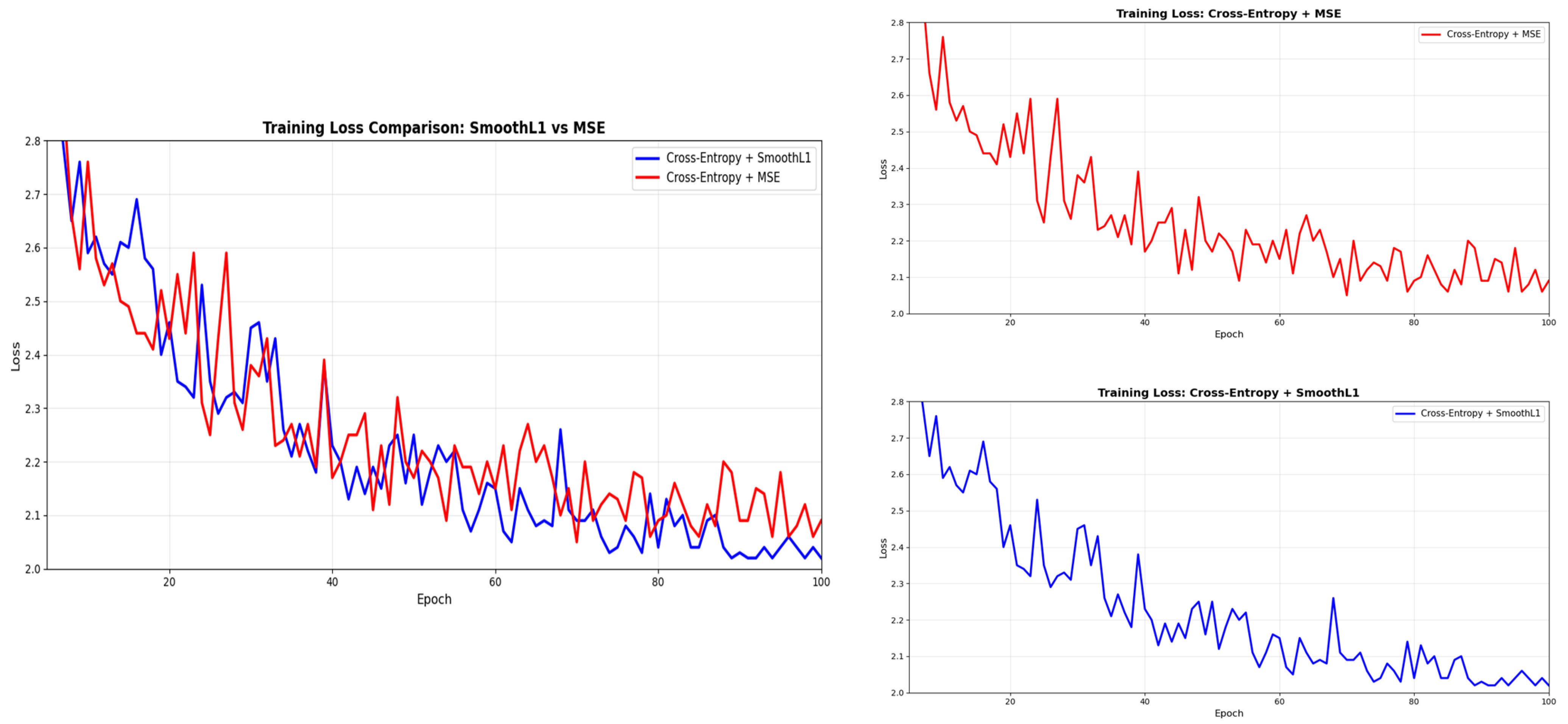
The experiment compares the loss function model from Reference 15 with the improved model proposed in this paper. The results are shown in Figure 6.

Experimental results demonstrate that the combination of Cross-Entropy and SmoothL1 loss functions exhibits superior convergence characteristics during training. Compared to the Cross-Entropy + MSE combination, Cross-Entropy + SmoothL1 achieved a lower final loss value of 2.02 cm after 100 training cycles while displaying a smoother and more stable convergence trajectory. The Cross-Entropy + MSE combination exhibited significant numerical fluctuations during the early training phase. This is attributed to the quadratic penalty characteristic of the MSE loss function for outliers, while the piecewise linear nature of the SmoothL1 loss function effectively mitigated gradient explosion issues. Thus, this result demonstrates that the SmoothL1 loss function selected in this paper reduces abrupt changes in model outputs, ensuring consistent predictions between adjacent frames. Consequently, it enables stable and smooth convergence for data featuring extreme head rotations and lighting conditions, enhancing the model’s robustness.

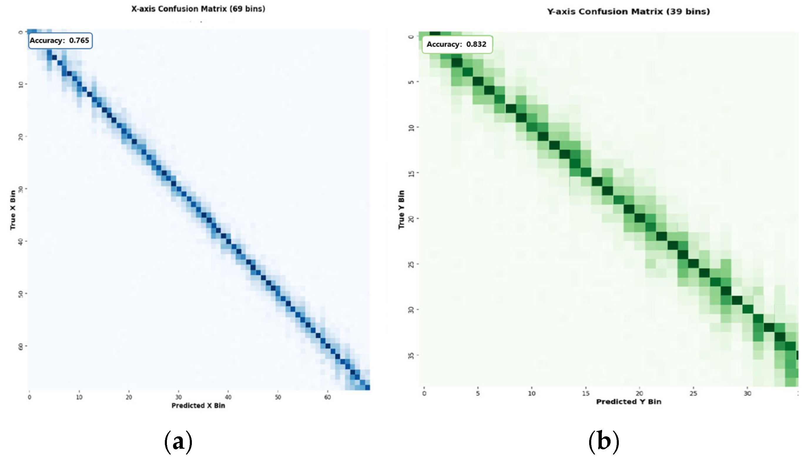
To validate the effectiveness of our coarse-to-fine fusion strategy, we first evaluate the classification branch’s ability to predict discrete grid bins. Figure 7 presents confusion matrices for both coordinate dimensions, showing.

The confusion matrix indicates that the classification branches successfully achieve coarse localization with an accuracy of 0.765 for the horizontal x category and 0.832 for the vertical y category, with prediction results highly concentrated along the diagonal. This demonstrates that the model accurately identifies the correct grid cell in most cases. Off-diagonal activations primarily occur in adjacent cells, a phenomenon consistent with expectations given the continuity of gaze movements and the 5-mm discretization interval.

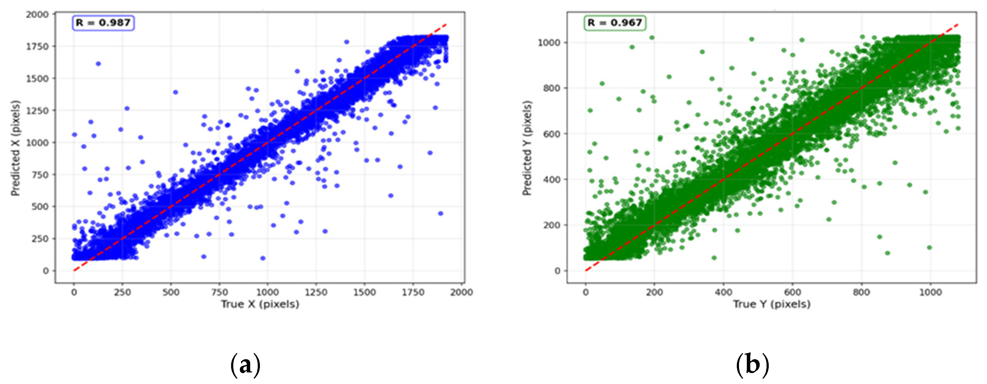
Based on coarse classification results, the regression branch performs fine coordinate optimization within predicted grid cells. Figure 8 displays scatter plots comparing final predicted coordinates with actual values after coarse-fine fusion.

The results show that the model’s predictions on both coordinate axes closely approach the ideal diagonal line x = y. The X-axis coordinate prediction achieved a correlation coefficient of 0.987, while the Y-axis coordinate prediction obtained a correlation coefficient of 0.967. Data points clustered tightly around the prediction line, indicating a strong linear correlation between predicted and actual values. The model maintained high accuracy across the entire coordinate prediction range, showing no significant systematic bias or prediction inaccuracies.

Additionally, we included several example prediction images in Figure 9. The images demonstrate that our improved model also delivers stable predictions for challenging examples (extreme lighting, dark environments), maintaining an error margin of approximately 2 cm.

4.4. Computational Efficiency Analysis

To evaluate the practical deployment feasibility of L1fcs-Net, we conducted a comprehensive computational cost analysis. The model architecture exhibits balanced complexity characteristics, making it suitable for real-time applications. The L1fcs-Net model contains a total of 28.16 million parameters, distributed across different components as follows:

This study conducted comprehensive performance evaluations on Alibaba Cloud’s GPU computing instance (configured with 8 vCPUs, 30GB memory, and NVIDIA A10 GPU). Experimental results demonstrate that the proposed model achieves a single-frame image inference time of 12 milliseconds, corresponding to a processing speed of 100 frames per second, fully meeting real-time processing requirements.

Furthermore, compared to other models in Table 1, our model achieves the best overall performance with a 12-millisecond inference time and 100 frames per second processing capability. This represents a 6.7–10× improvement over iTracker’s 10–15 fps, an 11.5× acceleration compared to GazeNets’ 138 ms inference speed, and a 4.17× increase over FullFace’s 50 ms processing speed. Moreover, the facial mesh branch introduced in Table 2 incurs only a minimal overhead of 0.08 GFLOPs (approximately 1.85% of the total computational load) while delivering significant accuracy gains, fully validating the efficiency of the dual-branch architecture.

4.5. Ablation Studies

To validate the effectiveness of each key component in the L2-2D-Net model, this paper conducted a comprehensive ablation study on the MPII-FaceGaze dataset, as shown in

Table 3. Melting Experiment Results.

Model	Initial Absolute Error	Final Absolute Error
Reg+Class (a)	4.19	2.17
Reg (b)	4.56	2.23
class (c)	6.08	2.19
Grid+Reg (d)	4.01	2.10
Grid+Class (e)	4.75	2.07

(a) Reg+Class (Gaze Point Classification and Gaze Point Regression) denotes a model incorporating both coarse gaze point classification and fine-grained gaze point regression components; (b) Reg (Gaze Point Regression) denotes a model containing only the fine-grained gaze point regression component; (c) Class (Gaze Point Classification) denotes a model containing only the coarse gaze point classification component; (d) Grid+Reg (Face Grids and Gaze Point Regression) is a model incorporating both the face grid branch and the gaze point fine regression component. (e) Grid+Class (Face Grids and Gaze Point Classification) is a model incorporating both the face grid branch and the classification coarse estimation component.

. These studies systematically analyzed the impact of the facial mesh branch, independent coordinate regression, independent classification estimation, and their combinations on model performance.

Experiments revealed that model (e) exhibited the smallest error, while model (b) showed the largest error. Additionally, all models incorporating facial mesh branches demonstrated superior accuracy compared to others. This indicates that the facial mesh branch enhances the network’s prediction of the face’s relative position to the gaze plane, thereby increasing the accuracy of gaze point prediction. Simultaneously, the experimental results demonstrate that adding a coarse classification estimation component significantly improves the network’s prediction precision.

5. Conclusions

Most current gaze point estimation models overly focus on gaze direction prediction while neglecting gaze point localization accuracy. Furthermore, methods mapping gaze direction to gaze points introduce cumulative errors from facial detection inaccuracies, and rigidly defined screen-to-face distances further degrade precision. These mapping computations also exhibit high computational complexity. To overcome gaze point estimation challenges, this paper proposes a gaze point estimation model that eliminates the need for additional mappings. By introducing facial mesh branches, the model projects the face relative to the screen, thereby obtaining distance and position information between the face and screen. Performance comparisons using classification and regression loss functions from the original model validate the improved performance, demonstrating that the proposed model effectively addresses the issue of insufficient gaze point estimation accuracy.

Furthermore, ablation experiments demonstrate that incorporating coarse-grained classification components significantly enhances network prediction accuracy. Consequently, further research on optimizing classification methods to improve gaze point estimation precision holds significant importance.

Future research directions will extend beyond computer monitor environments to encompass mobile devices such as smartphones and tablets. To account for scenarios like “gaze deviating from the screen,” the training phase incorporates gaze samples outside the screen; a binary classifier determines whether the gaze is within the screen boundary; and a post-processing threshold based on prediction confidence is implemented. As most modern mobile devices now feature RGB cameras suitable for eye-tracking technology, gaze estimation algorithms will serve a broader user base and diverse scenarios.