Multi-Source Feature Fusion Domain Adaptation Planetary Gearbox Fault Diagnosis Method

Abstract

To address the challenges of fault diagnosis in wind turbine planetary gearboxes under strong noise and limited labeled target-domain data, this paper proposes a novel intelligent diagnostic method integrating multi-source feature fusion with domain adaptation transfer learning. A Multi-source Feature Attention Fusion Convolutional Neural Network (MSFAF-CNN) is constructed, which dynamically fuses vibration signals from multiple measurement points using a channel attention mechanism to assign optimal weights to the most discriminative features. Furthermore, an improved Multi-source Local Maximum Mean Discrepancy (MS-LMMD) loss is introduced, establishing a hierarchical domain adaptation framework that enables fine-grained alignment of feature distributions between the labeled source and unlabeled target domains. Experimental results under the challenging condition of −4 dB noise demonstrate the superiority of the proposed approach: the cross-condition transfer task (A→B) achieves an accuracy of 95.32%, outperforming the conventional LMMD method by 1.05%. Finally, t-SNE-based visualization confirms that the method enhances cross-domain feature compactness, enabling direct processing of raw vibration signals without manual feature extraction. The findings indicate that the proposed approach offers a highly robust solution for fault diagnosis in drive systems under low signal-to-noise ratios and unlabeled operating conditions.

1. Introduction

In contemporary industrial systems, enhancing the precision of mechanical equipment fault diagnosis is paramount for ensuring production safety. Planetary gearboxes are extensively utilized in pivotal domains such as wind turbines [1] and construction machinery, due to their compact structure and high transmission ratio [2]. The operational stability of the transmission system and the service life of the equipment are directly determined by their health status [3]. When a planetary gearbox suffers from failures such as broken gear teeth or other similar problems, there is the potential for the transmission chain to fail, or indeed to lead to a major accident shutdown [4]. At present, the prevailing approach in this field is to diagnose faults based on gearbox vibration signals [5]. The Empirical Mode Decomposition (EMD) proposed by Huang et al. [6] provides an innovative tool for the analysis of non-linear vibration signals. Furthermore, frequency domain analysis based on the Fourier transform remains an invaluable tool in the identification of gearbox fault frequencies [7]. However, with the advent of breakthroughs in artificial intelligence technology, intelligent diagnostic methods represented by Machine Learning (ML) and Deep Learning (DL) are gradually becoming mainstream in the field of planetary gearbox fault diagnosis [8,9].

Convolutional Neural Networks (CNNs) have been shown to possess considerable advantages in the domain of intelligent fault diagnosis, due to their end-to-end feature-learning capabilities [10]. Zhang Wei et al. [11] pioneered the use of a wide convolution kernel structure to process raw one-dimensional vibration signals, combining Batch Normalization (BN) and Dropout regularization techniques to develop a Training Interference Convolutional Neural Network (TICNN) [12] with noise interference resistance capabilities. The Structure Optimized Deep Convolutional Neural Network (SOCNN) designed by Zheng Bo and Huang Jianhao et al. [13] demonstrates excellent robustness in gearbox transfer fault diagnosis under strong noise conditions through a multi-scale feature fusion mechanism [14]. Ye et al. [15] achieved adaptive optimal fusion of features through a dynamic weight allocation mechanism. This multi-source feature fusion method achieved by the dynamic weight allocation mechanism has achieved good results in fault diagnosis. Huang et al. [16] proposed a method for integrating feature and time-delay information from samples obtained via sliding window processing of multivariate time series. The resulting samples were then fed into the proposed CNN-LSTM model, comprising both CNN and LSTM layers, for diagnostic purposes.

In addition to continuous revisions to the main structure, ongoing innovations in convolutional neural network architecture have generated numerous lightweight add-on modules. The Parametric Rectified Linear Unit (PReLU) proposed by He Kaiming et al. [17] proposed the Parametric Rectified Linear Unit (PReLU), which replaces the traditional ReLU activation function with learnable parameters, thereby significantly enhancing gradient flow during backpropagation. Woo et al. [18] developed the Convolutional Block Attention Module (CBAM), Channel Attention Module (CAM), and Spatial Attention Module (SAM), whose collaborative mechanism enhances the model’s ability to extract features from fault-sensitive areas.

Addressing the practical challenge of data acquisition difficulties in industrial settings, transfer learning (TL) technology offers an effective solution for small-sample diagnostics [19,20]. Liu et al. [21] proposed a novel fault diagnosis approach based on incremental transfer learning and a selective ensemble of randomly configured networks. Residual convolutional denoising autoencoders and incremental transfer learning were employed for data preprocessing. An excellent ensemble learner was achieved using randomly configured networks (SCNs), mutual information, and parameter optimisation methods. Sun et al. [22] introduced multi-scale margin difference adversarial network transfer learning (MMDAN) for fault diagnosis. Multiscale neural networks extract rich features across domains, and a joint loss function is proposed to update neural network parameters. Two distinct case studies validate MMDAN’s effectiveness. Zhao et al. [23] guided by transfer learning principles, proposes two cross-domain aero-engine fault diagnosis methods: One-Stage Transfer Learning ELM (OSTL-ELM) and Two-Stage Transfer Learning ELM (TSTL-ELM). Both approaches are based on Extreme Learning Machines (ELMs), characterised by rapid training and robust real-time diagnostic capabilities. Domain adaptation (DA) techniques effectively address data distribution shifts between source and target domains [24]. Maximum Mean Discrepancy (MMD) [25], serving as a distribution divergence metric, achieves cross-domain feature space alignment through kernel function mapping [26]. By optimising the MMD loss function, the domain adaptation approach significantly enhances the diagnostic generalisation capability of planetary gearboxes under variable operating conditions.

In summary, the principal innovations of this paper may be summarised in the following three aspects:

(1)

Proposing a multi-source feature attention fusion mechanism based on ‘super-channel’ reconstruction, achieving dynamic weighting and complementary enhancement of vibration signals from multiple measurement points;

(2)

Proposing a multi-source local maximum mean difference loss function (MS-LMMD) to construct a hierarchical multi-source domain adaptation framework, enabling fine-grained alignment of multi-source data distribution discrepancies;

(3)

Developing an end-to-end planetary gearbox fault diagnosis system that maintains high accuracy and robust performance under conditions of strong noise and unlabelled target domains, demonstrating excellent engineering applicability.

2. Feature Extraction Model

2.1. MSFAF-CNN Model

This study uses vibration signals from planetary gearboxes as input, and is improved based on the Structural Optimization Convolutional Neural Network (SOCNN) framework to construct a Multi-Source Feature Attention Fusion Convolutional Neural Network (MSFAF-CNN) based on the Convolutional Block Attention Mechanism (CBAM). This architecture achieves adaptive weighted fusion of multi-source features based on the adaptive learning mechanism of CBAM, achieving efficient end-to-end classification from raw vibration signals to fault categories. The multi-source feature attention fusion convolutional neural network (MSFAF-CNN) is shown in Figure 1.

After one-dimensional vibration data is input into the model, a large convolution kernel measuring 64 is utilized to perform wide convolution in the initial layer. The use of a large convolution kernel in the first layer not only facilitates the extraction of short-term features, but also effectively extracts useful information from medium- and low- frequency vibration signals by expanding the model’s receptive field, and quickly reduces data length to avoid overly deep network structures. This is achieved by expanding the model’s receptive field, and simultaneously reduces data length to avoid overly deep network structures.

Subsequently, further feature extraction is performed using narrow convolutional kernels of sizes 1 and 3. The introduction of a multi-scale narrow convolutional kernel group through deep stacking realizes progressive extraction of deep abstract features. This multi-scale feature extraction strategy, by means of parallelizing convolutional channels with different receptive fields, can simultaneously capture multi-scale features of the signal. By combining with the CBAM attention mechanism, the extracted features are weighted using the Channel Attention Module (CAM) and Spatial Attention Module (SAM), thereby enabling the model to focus on parts that have a greater impact on diagnostic accuracy.

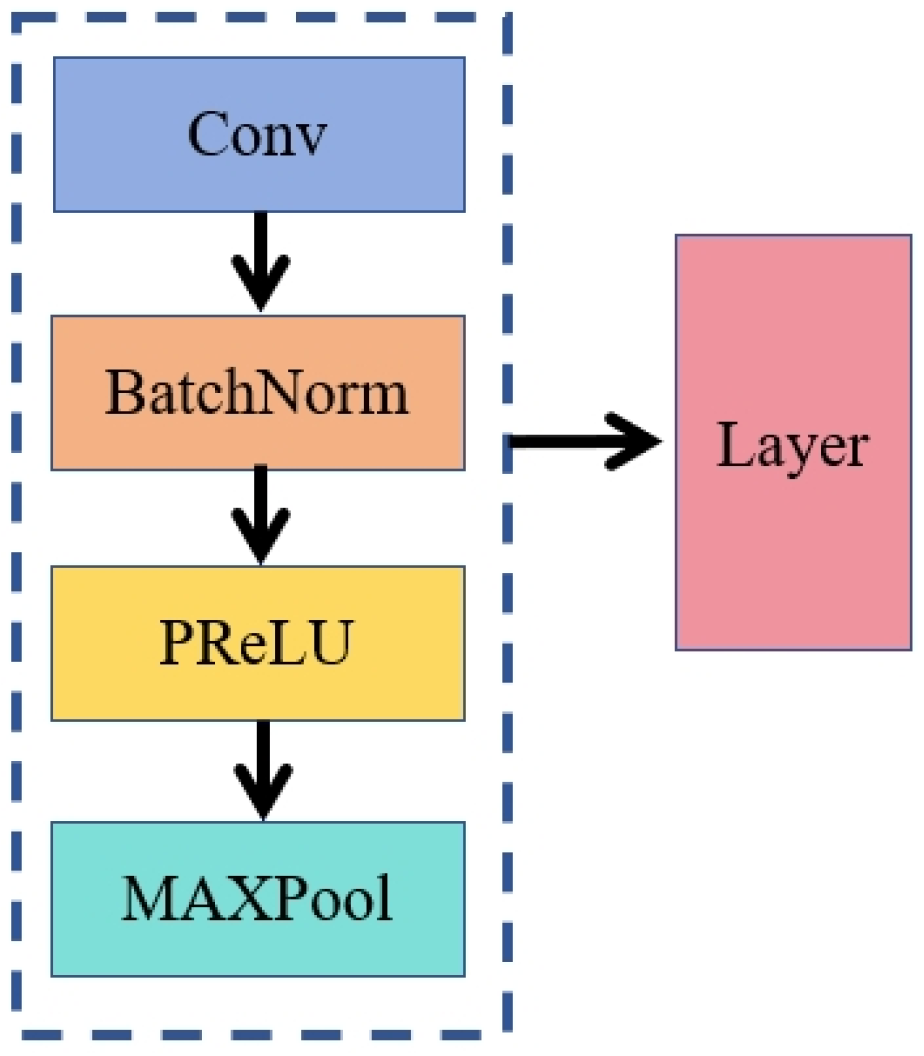
Furthermore, pooling operations are performed between each convolutional layer to reduce the spatial dimension of the feature map. Batch Normalization (BN) is used to regulate each layer, and parameterized rectified linear units (PReLU) substitute the conventional ReLU activation function, thereby mitigating the problem of neuron inactivation in the negative interval.

In conclusion, feature fusion is performed on multi-source heterogeneous data, and CBAM is applied to enable collaborative learning of heterogeneous data. In the feature dimension, the fusion weights of multi-source features are dynamically adjusted in an adaptive manner through backpropagation. It is evident that the feature expression layer utilizes a double-layer fully connected layer. Initially, the unfolded features are reduced to 100 neural nodes, and finally, a feature probability matrix for the number of fault types (classes) is output.

2.2. CBAM Attention Mechanism

The attention mechanism is designed to simulate the human attention process when identifying things. The efficacy of the model is enhanced by focusing on the information that needs attention while suppressing the interference from irrelevant information. Since its introduction, The attention mechanism has been quickly and widely applied in many areas of deep learning models, and has been continuously improved and optimized. This is due to its outstanding performance and simple, effective principles.

The Convolutional Block Attention Module (CBAM) is an efficient attention mechanism that has been widely applied to various two-dimensional images processing since its introduction. Following a series of modifications, the system has also exhibits excellent performance in one-dimensional data. CBAM consists of two independent sub-modules: the Channel Attention Module (CAM) and the Spatial Attention Module (SAM). By dynamically recalibrating the channel and spatial positions of feature maps, it enhances the model’s attention to key information while suppressing the interference from irrelevant information. The CBAM attentional mechanisms is shown in Figure 2.

In CAM, the channel attention module uses dual paths- global average pooling and global maximum pooling-to capture channel statistical features, so as to represent the mean of features and maximum value information, respectively. After the two types of features are fused via a shared multi-layer perceptron, the module generates channel weight vectors using a Softmax function. The calculation of the CAM is as follows:

$$M_C(f)=\sigma \left(MLP\left(MaxP\left(f\right)\right)+MLP\left(AvgP\left(f\right)\right)\right)$$

(1)

In the formula, f is the input data, $MaxP$ and $AvgP$ are maximum pooling and average pooling operations, MLP stands for multi-layer perceptron with shared weights, $\sigma$ is the Softmax activation function.

In the Spatial Attention Module (SAM), the module performs average and maximum pooling operations along the channel dimension to generate dual-channel spatial feature maps. After filtering with a 7-sized convolution kernel and performing the Softmax activation operation, the module outputs the spatial weight matrix. The calculation formula for SAM is as follows:

$$M_S(f_C)=\sigma \left(Con{v}_{(7)}\left(C\left[AvgP\left(f_C\right),MaxP\left(f_C\right)\right]\right)\right)$$

(2)

In the formula, $f_C$ is the weighted feature data after CAM processing, $C$ is the operation of concatenating two pooled features,$Conv$ is a one-dimensional convolution with a kernel size of 7.

In the MSFAF-CNN model, the CBAM attention mechanism is applied to multi-scale convolutional structures and multi-source feature fusion. It allocates weights to the feature channels and spatial dimensions derived from the combination of branch results, thereby enhancing the model’s focus on important features and further improving its noise resistance performance and accuracy.

2.3. Batch Normalization and Prelu Activation Function

Batch Normalization (BN) [23] is a technique for processing the outputs of network nodes during forward propagation, and is typically placed before the activation function to address the issue of internal covariate shift during training. At its core, batch normalization normalizes the outputs—i.e., adjusts the output values of each node—so that these values have a distribution with a mean of 0 and a variance of 1, thereby ensuring a stable distribution. Batch normalization has two primary objectives. Firstly, it optimizes the network training process by normalizing input features, reducing dependence on initialization, and enabling easier learning and convergence. Secondly, it exerts a certain degree of regularization effect, thereby reducing the risk of overfitting.

PReLU is an improved version of the ReLU activation function, designed to address the problem of vanishing gradients for negative inputs. The ReLU function is a widely popular nonlinear activation function that outputs the input value directly for non-negative inputs and 0 for negative inputs. This property makes ReLU highly effective in training deep neural networks, as it mitigates vanishing gradients and accelerates the training process. However, a disadvantage of ReLU is that when the input is negative, the gradient is zero, which can lead to the ‘death’ of neurons—meaning that they no longer respond to any subsequent training data. The application of PReLU in the convolutional module of each layer is demonstrated shown in Figure 3.

PReLU addresses this issue by introducing a learnable parameter. For negative inputs, PReLU does not simply set them to 0, but multiplies them by a small positive coefficient (i.e., slope), which is learned during the model training process. Therefore, the expression for PReLU can be written as follows:

$$PReLU\left(x\right)=\left\{\begin{array}{c}x,x>0\\ ax,x\le 0\end{array}\right.$$

(3)

Among them, $x$ is the input, $PReLU\left(x\right)$ is the output, $a$ is the slope parameter learned separately for each neuron. During the training process, the network assimilates these slope parameters, thereby ensuring the production of non-zero gradients even in the presence of negative inputs. This capacity to circumvent the phenomenon of neuronal death is a significant advancement in the field.

In this model, PReLU is used to replace ReLU and is placed after each batch normalization layer that following convolution. This ensures that the network can learn more complex feature representations.

2.4. Optimization of One-Dimensional Convolutional Neural Network Structures

The structural optimization of one-dimensional convolutional neural networks primarily involves the first-layer wide convolution architecture and multi-scale convolution strategies. The primary feature of the first-layer wide convolution is the use of a large-scale kernel of size 64 in the initial layer. This design enhances the network’s receptive field to achieve effective extraction of key information from medium- and low-frequency vibration signals [27]. Its working mechanism shares similarities with the short-time Fourier transform, thus allowing the architecture to capture the local time-frequency characteristics of signals. These trainable large-scale kernels, which can be trained via gradient optimization, autonomously mine diagnostic-related features, significantly improving the accuracy of signal classification and computational efficiency. This architecture reduces network depth to conserve computational resources while maintaining its excellent performance, and has now become the standard configuration for one-dimensional convolutional models.

Multi-scale convolutional neural networks refer to neural networks that extract features using multiple convolutional kernels of different scales and sizes. These convolutional kernels have distinct receptive fields, thus allowing them to capture image features across multiple scales. Shorter kernels focus on extraction short-term dependencies in sequences. and high-frequency features. In contrast, longer kernels can capture long-term dependencies and low-frequency features. By combining these kernels of different lengths, the model can generate rich feature representations across multiple scales, thereby enhancing its ability to understand signal features at multiple scales.

In this model, the first-layer wide convolution and two multi-scale branch layers are adopted for the data construction of each channel. By performing convolution and pooling on feature data using kernels of different sizes, the model retains the diversity of feature extraction from the multi-scale branch layers while generating output feature maps of identical size. These feature maps are then merged along their channels and outputted. The multi-scale convolution layer structure for each channel is illustrated in Figure 4. In the figure, “Conv(x) × y” represents the convolution kernel size is x, one-dimensional convolution operation with output channel count y, “MaxP(x)” is the maximum pooling, “AvgP(x)” is the average pooling, in “CBAM(y)”, y represents the number of input and output channels.

2.5. Multi-Source Feature Fusion Method

Multi-source feature fusion for one-dimensional vibration signals refers to the integration of multiple related one-dimensional data samples collected at the same time, aiming to implement a multi-source data collaborative analysis method for target identification. Multi-source fusion can be categorized into three levels: data-level fusion, directly fuses raw data through concatenation or weighting to preserve complete information, but requires high storage and computational costs; feature-level fusion, which concatenates and weights extracted features to balance information preservation and data compression, and achieves the best overall performance; decision-level fusion, which integrates classification results through voting or weighted averaging, and has strong fault tolerance but incurs significant information loss.

As powerful feature extractors, one-dimensional convolutional neural networks can achieve feature-weighted concatenation by applying CBAMs. First, the network performs data flattening to expand the features of each data sample into a ‘super channel’—i.e., merging one-dimensional features with the channel dimension. Next, the CBAMs perform channel and spatial attention targeting each ‘super channel’. Finally, the network splits the ‘super channels’ and fed into the classification layer. This process treats the features extracted from each heterogeneous data sample as a channel to allocate weights, and achieves the focus on the key features of each data sample via spatial attention.

Feature fusion methods can process data from multiple acquisition channels and combine information from these channels. This makes them highly robust to noise or outliers in single-channel data. Furthermore, integrating information from different channels enables the model to learn richer and more diverse feature representations, thereby enhancing its generalization performance.

The method that combines multi-scale convolution and multi-source feature fusion comprehensively captures the intrinsic features of the data, as well as the unique information from the different channels, by combining information from various scales and data from multiple acquisition channels. This enables the model to obtain a more complete and accurate data representation, thereby improving its ability to extract fault features and identify noisy data.

3. Domain Adaptation Loss Function

3.1. Cross-Entropy Loss Function

Cross-Entropy Loss (CEL) is a widely used loss function in the field of machine learning, especially for classification tasks. It quantifies the discrepancy between a model’s predicted output and the true labels, and optimizes the model by minimizing this discrepancy.

In multi-class classification tasks, the model typically outputs predicted probabilities for each class. These probabilities are derived via the Softmax function, which ensures the sum of predicted probabilities across all classes equals 1. The true label ${\mathit{y}}_i$ is a one-hot encoded vector in which only one element is 1, indicating the class the sample belongs to and the remaining elements are 0. The cross-entropy loss function can be expressed as follows:

$$Los{s}_{CEL}=-{\displaystyle \sum _{i=1}^C{\mathit{y}}_i\log \left({\widehat{\mathit{y}}}_i\right)}$$

(4)

In the formula, ${\widehat{\mathit{y}}}_i$ is the probability prediction matrix, $C$ is the number of sample types.

This paper uses the cross-entropy loss function to train the source domain using labelled data.

3.2. Local Maximum Mean Difference

In transfer learning, domain adaptation methods are effective approaches to address the unlabeled problem of the target domain and enhance the model’s generalization ability on the target domain, thereby achieving effective transfer learning. A classic domain adaptation method employs the Maximum Mean Distance (MMD) between source and target domain features as the loss function. MMD is commonly used in machine learning and transfer learning to measure the distance between two different but related distributions. The MMD loss function assesses the discrepancy between two distributions by comparing their higher-order moments or the mean differences after feature mapping. The formula for the MMD loss function is as follows:

$$\begin{array}{ll}Los{s}_{MMD}& ={‖{\displaystyle \frac{1}{n}}{\displaystyle \sum _{i=1}^n\varphi }(x_i)-{\displaystyle \frac{1}{m}}{\displaystyle \sum _{j=1}^m\varphi }(y_j)‖}_2^H\\ & ={\displaystyle \frac{1}{n^2}}{\displaystyle \sum _{i,j=1}^{n}K(x_i,x_j)}+\hspace{0.17em}\hspace{0.17em}\hspace{0.17em}{\displaystyle \frac{1}{m^2}}{\displaystyle \sum _{i,j=1}^{m}K(y_i,y_j)}\\ & \hspace{0.17em}\hspace{0.17em}\hspace{0.17em}-{\displaystyle \frac{2}{nm}}{\displaystyle \sum _{i=1}^n{\displaystyle \sum _{j=1}^{m}K(x_i,y_j)}}\end{array}$$

(5)

In the formula,$x_i$ and $y_j$ are elements from two samples with different distributions, ∅(∙) is a mapping function, $n$ and $m$ are the sizes of the sets, $K(x,y)$ is a Gaussian kernel function, i.e., an RBF kernel function, as shown in the following formula:

$$K(x,y)=\exp \left(-{\displaystyle \frac{|x-y{|}^2}{2{\sigma }^2}}\right)$$

(6)

In the formula, $\sigma$ is the bandwidth parameter, which controls the smoothness of the kernel function.

Although MMD can reduce the overall distribution discrepancy between the source and target domains as a global domain adaptation method, it ignores the subdomain differences among specific fault categories. This causes the boundaries between subdomains, potentially leading to the misclassification of similar fault features into distinct subdomains and thus increasing the risk of diagnostic errors.

To overcome this challenge, scholars have proposed the Local Maximum Mean Discrepancy (LMMD) method [28]. While preserving the global distribution alignment capability, LMMD introduces category label information from the target domain to construct a hierarchical feature alignment framework. This achieves subdomain adaptation based on data categories. This optimization strategy enables the model to maintain its ability to generalize across domains while significantly improving the distinguishability of subdomain boundaries, which in turn improves the confidence of fault diagnosis and its robustness across varying operating conditions.

To minimize the class distance of corresponding subclasses, LMMD adds the weights belonging to each class and calculates their unbiased estimates, i.e., it adds various mathematical expectations as a whole. The LMMD loss function formula can be expressed as follows:

$$\begin{array}{ll}Los{s}_{LMMD}& ={\displaystyle \frac{1}{C}}{\displaystyle \sum _{j=1}^C{‖{\displaystyle \sum _{i=1}^n{\omega }_i^s\varphi }(x_i)-{\displaystyle \sum _{j=1}^m{\omega }_j^t\varphi }(y_j)‖}_H^2}\\ & ={\displaystyle \frac{1}{C}}{\displaystyle \sum _{j=1}^C\left[{\displaystyle \sum _{i,j=1}^n{\omega }_i^s{\omega }_j^{s}K(x_i,x_j)}+\hspace{0.17em}\hspace{0.17em}\hspace{0.17em}{\displaystyle \sum _{i,j=1}^m{\omega }_i^t{\omega }_j^{t}K(y_i,y_j)}\right.\hspace{0.17em}\hspace{0.17em}\hspace{0.17em}}\\ & \hspace{1em}\hspace{1em}\hspace{1em}\hspace{1em}\left.-2{\displaystyle \sum _{i=1}^n{\displaystyle \sum _{j=1}^m{\omega }_i^s{\omega }_j^{t}K(x_i,y_j)}}\right]\end{array}$$

(7)

In the formula, $C$ is the number of label categories in the dataset, $s$ represents the source domain, $t$ represents the target domain, ${\omega }^s$ and ${\omega }^t$ represent the weights of corresponding classes in $x_i$ and $y_j$, respectively, and are calculated using the following formula:

$${\omega }_i={\displaystyle \frac{Z_{ic}}{{\displaystyle {\sum }_{(x_j,y_j)\in D}{Z}_{jc}}}}$$

(8)

In the formula, $D$ is the sample space of the data set, $Z_{ic}$ is the probability of the sample under the category. This probability is a single hot label in the source domain and a probability prediction matrix output by the model in the target domain.

In domain adaptation-based transfer learning methods, the LMMD method is adopted to compute the domain adaptation loss function. Through local alignment and weighted calculation, it can effectively align the feature distributions of the source and target domains in transfer learning, capture the distribution discrepancies between the two domains more accurately, thereby enhance the model’s generalization capability and performance to realize the transfer process.

3.3. Multi-Source Local Maximum Mean Difference

In deep learning-based transfer learning methods, applying multi-layer MMD to measure feature distribution discrepancies across different network layers enables hierarchical modelling of cross-domain feature alignment [19]. This approach captures multi-granularity feature shifts from shallow to deep layers, which not only enhances the model’s capability to characterize distribution discrepancies but also improves the robustness of feature transfer via a hierarchical optimization strategy.

However, existing multi-layer MMD methods and their improvements only consider feature fusion, without taking the specificity of different measurement points and directional data into account. This makes it difficult to handle the specific features of each measurement point in multi-source data effectively. Building on the improved Local Maximum Mean Difference (LMMD), this paper proposes the Multi-source Local Maximum Mean Difference (MS-LMMD) method.

The core innovation of MS-LMMD lies in constructing a pre-measurement-point domain adaptation mechanism. Prior to the feature fusion layer, this method performs LMMD calculations separately in the feature space of each measurement point, thereby accurately evaluating the cross-domain distribution discrepancies of channel-specific features. LMMD loss terms are constructed both in the feature space of each measurement point and in the fused fully connected layer. Dynamic weight assignment is implemented based on the number of measurement points and the CAM weights of the ‘super channels’ in the CBAM attention mechanism. The loss function is constructed as shown below:

$$Los{s}_{MS-LMMD}={\displaystyle \sum _{i=1}^B{a}_{i}Los{s}_{LMM{D}_i}+Los{s}_{LMM{D}_{total}}}$$

(9)

In the formula, B represents the total number of measurement point channels, $Los{s}_{LMM{D}_i}$ represents the LMMD loss value at each measurement point, i is the index of the test data channel, $Los{s}_{LMM{D}_{total}}$ is the feature space difference loss after the fusion layer.

For weight assignment, the channel weights of “super channels” are derived from the CBAM model during feature fusion. Since the final Softmax activation function in CAM ensures the sum of weights is always 1, the initial weights are set to 1/B. As the number of measurement points increases, the weight for each individual measurement point decreases automatically, which effectively avoids the suppression of the loss term in the feature fusion layer caused by loss value inflation in multi-channel scenarios. The LMMD loss of each measurement point not only characterizes the distribution shift in the specific feature space but also complements the global loss of the fusion layer, jointly depicting the heterogeneous characteristics of multi-source data. During the calculation, the source domain label information and the target domain feature probability prediction matrix must be input simultaneously. The specific data flow is shown in Figure 5.

The weighting values are distributed using an equal weighting method, averaging the LMMD across each branch channel. As the volume of test data within the hierarchy increases, the proportion of each individual loss value within the overall loss correspondingly diminishes. This adjustment mechanism aims to prevent the loss function value from abnormally escalating due to excessive channels, thereby obscuring or neglecting the contribution of the LMMD loss term following feature fusion. Building on the fine-grained alignment advantages of LMMD, the MS-LMMD method innovatively constructs a domain adaptation framework for multi-source data. By synergistically optimizing measurement point specificity and global commonality, it significantly enhances the model’s diagnostic stability under multi-source heterogeneous data and variable operating conditions. It demonstrates particularly strong feature decoupling capabilities when processing vibration signals with spatial distribution differences.

The domain adaptation loss function is combined with the classification loss function to form the total network loss; task learning is achieved by minimizing this loss. This paper proposes a composite loss function for domain adaptation transfer learning by combining CEL and MS-LMMD loss, achieving unsupervised fault identification of the planetary gearbox in the target domain.

3.4. Introducing Gaussian White Noise

The introduction of Gaussian white noise serves as a composite simulation of these complex noise characteristics. With its relatively uniform power spectral density across specific frequency ranges and stationary random properties, Gaussian white noise can statistically encompass certain combined effects of different noise types such as mechanical and electrical noise. This approach enables the simulated noise environment to better approximate the actual noise interference conditions encountered in wind turbine operations.

During the noise addition process, the Signal-to-Noise Ratio (SNR) serves as a crucial metric for quantifying signal strength relative to noise intensity. The SNR formula is expressed as follows:

$$SNR\left(dB\right)=10\cdot log10\hspace{0.17em}({\displaystyle \frac{P_{signal}}{P_{noise}}})$$

(10)

where $P_{signal}$ represents the signal power and $P_{noise}$ denotes the noise power.

According to the maximum entropy theorem under power constraints in Shannon’s information theory, a Gaussian-distributed signal source achieves maximum entropy under average power constraints, indicating that noise uncertainty reaches its peak and causes the most significant interference to the signal source at this point. In the field of fault diagnosis, Gaussian white noise, with its maximum uncertainty characteristics, can effectively simulate noise environments approaching real-world complex conditions, thereby thoroughly testing and evaluating the robustness and effectiveness of diagnostic methods.

Within the fault diagnosis domain, academic consensus generally regards the addition of Gaussian white noise with SNR ≤ 0 dB as representative of strong noise environments. To validate the noise resistance performance of diagnostic models under noisy conditions, additional Gaussian white noise at five intensity levels (−6 dB, −4 dB, −2 dB, 0 dB, and 2 dB SNR) was introduced to the original vibration signals. These noise levels span from extremely harsh to relatively favorable conditions, effectively simulating various noise interference scenarios encountered in practical operational environments. Training models with noise-contaminated data facilitate comprehensive evaluation of the noise immunity of data-driven fault diagnosis methodologies.

4. Experimental Setup

4.1. Validation Dataset and Preprocessing

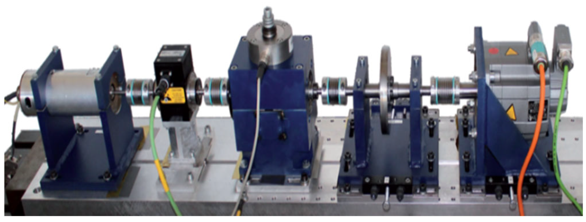
The experimental data used in this paper were selected from the WT planetary gearbox dataset, which was compiled and released by a team led by Liu Dongdong and Cui Lingli at Beijing University of Technology, in collaboration with researchers including Cheng Weidong at Beijing Jiaotong University [29]. The dataset comprises vibration data collected from a planetary gearbox within a *wind turbine transmission system experimental apparatus, the structure of which is depicted in Figure 6.

The experimental setup comprises a drive motor, a planetary gearbox, a fixed shaft gearbox and a loading module. A Sinocera CA-YD-1181 accelerometer is used to collect vibration signals, while an encoder simultaneously obtains speed pulses. In the transmission experimental setup, the planetary gearbox comprises four planetary gears that rotate around a sun gear.

The WT planetary gearbox dataset from Beijing, China, contains operational data from five planetary gears under eight rotational speed conditions: 20 Hz, 25 Hz, 30 Hz, 35 Hz, 40 Hz, 45 Hz, 50 Hz, and 55 Hz. This dataset provides a foundation of data for cross-domain diagnostic research under varying operating conditions. At a sampling frequency of 48 kHz, five minutes of data were collected for each operating state and rotational speed, ensuring sufficient data volume. Additionally, vibration signals in the x and y directions were collected simultaneously, paving the way for multi-source fusion fault diagnosis methods to be applied.

To test the model’s noise resistance based on the maximum entropy theorem under power constraints in Shannon’s information theory, the entropy value of a Gaussian-distributed signal source is maximized under average power constraints. This indicates that noise uncertainty is strongest and the interference it causes to the signal source is most significant at this point. Additional Gaussian white noise with signal-to-noise ratios (SNR) of −4 dB, −2 dB, 0 dB, 2 dB and 4 dB was added to the original vibration signal in order to simulate challenging yet realistic strong-noise scenarios in real-world industrial conditions. This range was selected as it represents the severe noise levels realistically encountered in wind turbine operations, based on our analysis of field data and relevant literature. Testing within this range ensures the evaluation is both rigorous and practically meaningful.

The statistics for various operating conditions in the WT dataset are shown in

Table 1. Table of data types in WT- datasets.

Operating Conditions	Data Types
status	health status/0, tooth surface wear/1, tooth damage/2, tooth fracture/3, tooth loss/4
channel	x, y
speed	20 Hz, 25 Hz, 30 Hz, 35 Hz, 40 Hz, 45 Hz, 50 Hz, 55 Hz
noise	−4 dB, −2 dB, 0 dB, 2 dB, 4 dB

.

Add simulated noise environments comprising Gaussian white noise at the aforementioned five intensities. For each dataset, partition 300 samples of one-dimensional acceleration data, each comprising 2048 sampling points. The data comprised one healthy state and four fault states. To prevent data leakage, the entire sample set for each fault state and channel was divided chronologically into a training set (the first 90% of samples, i.e., 270 samples per state per channel) and a test set (the final 10%, i.e., 30 samples per state per channel), ensuring no temporal overlap between the two sets. For each operating condition, data from both x and y channels were collected, with data from both directions treated as a single group. Based on the WT planetary gearbox dataset, the data were partitioned into two distinct subsets characterized by relatively higher and lower rotational speeds, as detailed in

Table 2. Variable operating condition transfer learning dataset.

Dataset	Number of Data Samples for Each Type	Faults Types	Speed (Hz)
A	300	5	20, 25, 30
B	300	5	40, 45, 50

.

To ensure the reproducibility and comparability of experimental results, all data partitioning processes—including the chronological split of each fault state and channel into training and testing sets—were performed using a fixed random seed. Similarly, the batch sampling order during model training was also controlled by a fixed random seed. After partitioning, Gaussian white noise was added to the original signals at various signal-to-noise ratios (SNR) to simulate different noise environments. This approach ensures that the original signal conditions remain consistent across different noise levels, thereby enhancing the comparability of model performance under varying noise intensities.

4.2. Comparative Experimental Setup

Two types of comparison experiment were set up to verify the robustness and superiority of the proposed MSFAF-CNN model and MS-LMMD method in noisy environments.

(1)

Feature extraction model comparison experiment

TICNN (Traditional Interference Convolutional Neural Network) [11]: Represents the benchmark performance of traditional convolutional neural networks in the task.

SOCNN (Structural optimisation achieved by integrating multi-scale convolutions with the broad convolutional approach) [13]: As a cutting-edge research achievement, the model has undergone structural optimization.

SOCNN-CBAM (Introducing Attention Mechanism): Based on multi-scale convolution, the CBAM attention mechanism is added after two layers of multi-scale structure.

MS-SOCNN (multi-source SOCNN): Directly performs multi-source data splicing based on SOCNN without applying the CBAM.

MSFAF-CNN (a novel multi-source data attention fusion network proposed in this study): By transforming data into ‘super channels, CBAM attention is applied to perform weighted fusion of multi-source data.

(2)

Domain adaptation migration experiment

MSFAF-CNN (CEL): Trained using cross-entropy loss.

MSFAF-CNN (LMMD): A method based on local maximum mean difference for traditional subdomain-adaptive transfer learning.

MSFAF-CNN (MS-LMMD): Based on the proposed multi-source data fusion structure, multi-source subdomain adaptation transfer learning is performed using an improved MS-LMMD loss function.

In the context of model training, the training and testing processes for all datasets were implemented using the PyTorch 2.6 deep learning framework, which is based on Python 3.9. The training hyperparameters were set as follows: batch size batch_size = 50, learning rate lr = 0.001, Adam optimiser, and 250 epochs.

The outcomes of the aforementioned comparison experiments not only verify the robustness and superiority of the MSFAF-CNN model in noisy environments, but also reveal the important role of the MS-LMMD domain adaptation strategy in improving its performance.

4.2.1. Comparison of Feature Extraction Model Performance

In order to eliminate the impact of randomness in deep neural network parameters on evaluation results, this study adopted a five-round independent experiment verification mechanism. Within the confines of fixed hyperparameter conditions, the network weights underwent a reinitialization process in each experimental iteration. The arithmetic mean was then employed as the metric to assess the final performance of the model. The results of the study are presented in

Table 3. Average accuracy of each method.

Network Model	Data Channel	Average Accuracy Rate (%)
		−4 dB	−2 dB	−0 dB	2 dB	4 dB
TICNN	x	89.67	92.89	94.11	96.19	97.33
	y	92.89	94.31	96.89	97.28	99.04
SOCNN	x	93.25	94.67	95.15	96.32	97.89
	y	95.24	97.33	98.14	98.85	99.33
SOCNN-CBAM	x	94.56	96.14	97.56	98.11	98.21
	y	96.76	98.25	99.14	99.35	99.71
MS-SOCNN	x , y	98.56	99.07	99.67	99.89	100
MSFAF-CNN	x , y	99.04	99.45	99.83	100	100

.

In the single-channel model, the multi-scale structure SOCNN demonstrates a substantial enhancement over TICNN, exhibiting a 3.58% increase in accuracy at the x-channel −4 dB level. It is evident that SOCNN-CBAM demonstrates a substantial enhancement in performance when compared with the base SOCNN. As the level of noise increases, the benefits of the attention mechanism become more evident. At the x-channel −4 dB noise level, an improvement in accuracy from 93.25% to 94.56% (+1.31%) was observed, and a corresponding increase in the accuracy of the y channel from 95.24% to 96.76% (+1.52%) was also noted.

MS-SOCNN attains an accuracy rate of 98.56% at −4 dB through dual-channel direct concatenation, signifying a 1.80% enhancement over the single-channel optimal SOCNN-CBAM (y-channel 96.76%), thereby underscoring the complementary value of multi-source data. Meanwhile, MSFAF-CNN employs ‘super channel’ reconstruction combined with CBAM fusion, further improving accuracy at −4 dB to 99.04%, an increase of 0.48% over MS-SOCNN, and achieving 100% stable diagnosis in conditions above 2 dB.

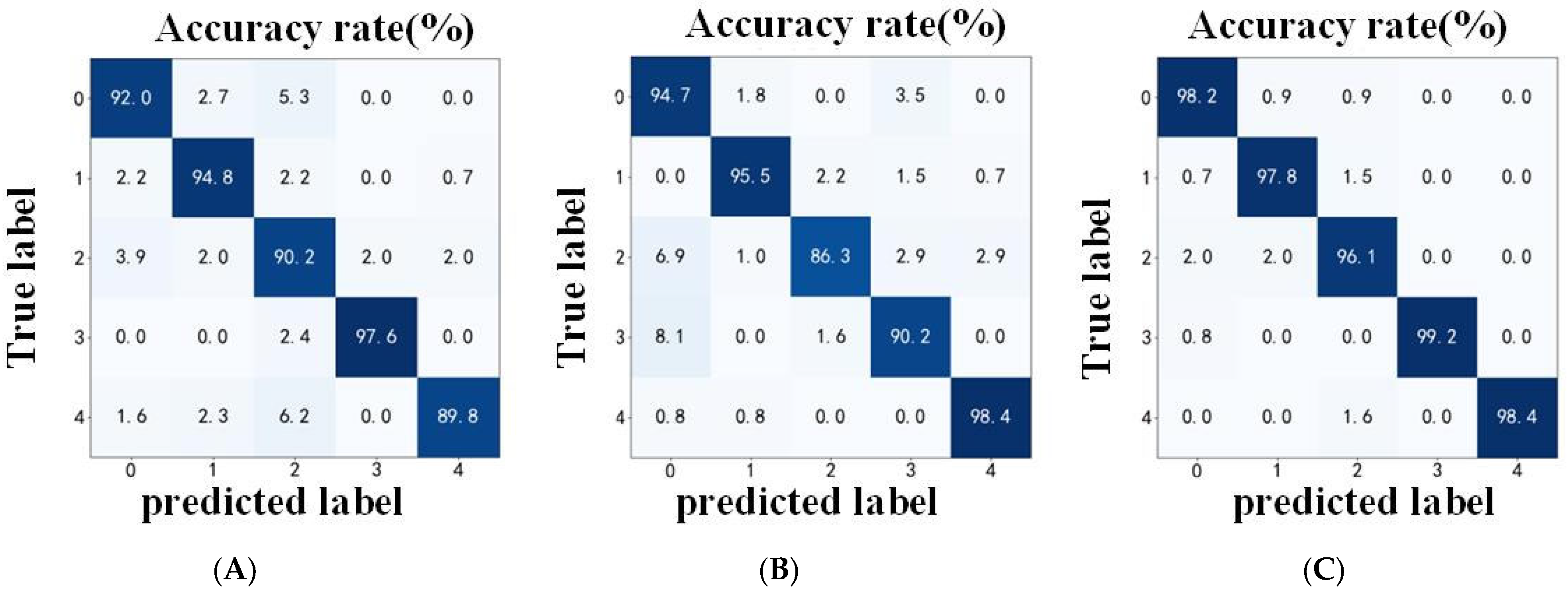
In order to more intuitively demonstrate the synergistic optimization effect between single-channel and multi-channel models, the confusion matrices of the two channels of SOCNN-CBAM at −4 dB are compared with those of MSFAF-CNN, as illustrated in Figure 7.

In the confusion matrices for each channel method, along the x-axis, the fault recognition accuracy for labels 2 and 4—namely tooth damage and tooth loss conditions—stands at 90.2% and 89.8%, respectively, both below the overall accuracy of 91.03%. This indicates that x-channel data presents greater recognition challenges for these two categories. Along the y-axis, faults labelled 2 and 3—tooth defects and tooth fractures—fell below the overall average accuracy of 92.04%. However, accuracy for label 4 (tooth missing) reached 98.4%, significantly outperforming x-axis data. Thus, despite minimal difference in overall average accuracy, each channel’s data clearly exhibits distinct advantages for different faults.

The high accuracy of MSFAF-CNN diagnostic results is attributable to its core technology, which suppresses noise features through channel attention, reinforces the location of key vibration segments through spatial attention, distinguishes the influence of multiple data sources in diagnosis, and applies multiple data sources for collaborative optimization, ultimately improving the model’s accuracy.

4.2.2. Performance Comparison of Transfer Learning Methods

In accordance with the domain adaptation comparison experiment settings outlined above, the proposed model and method were subjected to training and testing, and the accuracy of the transfer learning target domain was subjected to statistical analysis. Each experiment was conducted on five occasions, and the mean value was calculated. The specific results are displayed in

Table 4. Comparison of average accuracy of migration learning.

Migration Direction	Loss Function Method	Average Accuracy Rate (%)
		−4 dB	−2 dB	0 dB	2 dB	4 dB
A→B	CEL	78.35	80.54	79.78	81.24	82.56
A→B	CEL + 0.5 LMMD	94.27	96.28	97.68	98.58	98.95
A→B	CEL + 0.5 MS-LMMD	95.32	96.54	97.95	98.78	99.21
B→A	CEL	78.65	79.67	80.67	81.51	83.37
B→A	CEL + 0.5 LMMD	95.78	96.34	97.56	98.36	98.85
B→A	CEL + 0.5 MS-LMMD	96.04	96.67	97.91	98.59	99.11

.

The investigation into the mean accuracy rate in the context of domain adaptation transfer experiments revealed that the fundamental cross-entropy loss (CEL) exhibited an average accuracy rate that fell short of 84% for all levels of noise in transfer learning. This outcome was found to be considerably lower than those of the subsequent two methods. Following the introduction of the LMMD method, the accuracy rate in the A→B direction increased from 94.27% to 98.95%, while the accuracy in the B→A direction increased from 95.78% to 98.85%. The multi-source improved MS-LMMD method further optimized the transfer performance, maintaining the highest possible level of accuracy under all noise conditions. A comparative analysis with the conventional LMMD approach revealed an average enhancement ranging from 0.5% to 1.2%, underscoring enhanced noise resilience and operational adaptability.

In order to visualize the feature layer output for the migration task from source domain A to target domain B, under the scenario in which the lowest average accuracy of migration learning at a signal-to-noise ratio of −4 dB was achieved, t-SNE dimensionality reduction was employed, as illustrated in Figure 8.

The feature dimension reduction diagram demonstrates that when the CEL method is employed in the source domain alone, multiple labels become intermingled. This indicates that a single classification loss is inadequate in overcoming inter-domain distribution differences. The CEL + LMMD approach has been shown to achieve subdomain alignment through the utilization of local maximum mean differences, thereby significantly enhancing the model’s generalization capability. This outcome serves to demonstrate the effectiveness of domain adaptation strategies in matching feature distributions. The CEL + MS-LMMD model incorporates a multi-source data fusion mechanism, thereby facilitating more precise domain- invariant feature extraction across a range of operating conditions. The reduced-dimension features exhibit enhanced cohesion, with clearer boundaries.

In order to verify the stability of the transfer learning method, the standard deviation of the accuracy rates for five training sessions in a −4 dB noise scenario was calculated. The results of this calculation are shown in

Table 5. Standard deviation of various methods.

Loss Function	Standard Deviation in the A→B Direction	Standard Deviation in the B→A Direction
CEL	2.33%	2.17%
CEL + 0.5 LMMD	0.74%	0.69%
CEL + 0.5 MS-LMMD	0.51%	0.54%

.

Table 5 illustrates that the conventional CEL method is deficient in domain adaptation mechanisms, leading to substantial noise interference during training and a standard deviation that is considerably higher than that of domain adaptation methods. LMMD enhances model robustness through subdomain alignment constraints, but MS-LMMD, which uses multi-source optimization, performs better in terms of consistency in the direction of transfer, confirming the strengthening effect of multi-source feature fusion on training stability.

Using the test accuracy at the −6 dB threshold—where model performance differences are most pronounced—as the performance metric, we analyzed the performance and computational overhead of feature-extraction models on the laboratory dataset. The results are shown in

Table 6. Model performance and computational overhead.

Model Name	Used Data	Accuracy	Training Time	Testing Time	Average Time per Sample
WDCNN	1 channel	84.34%	10 min 24 s	21 s	19.44 ms
SOCNN	1 channel	84.48%	11 min 32 s	22 s	20.37 ms
SOCNN-CBAM	1 channel	87.45%	12 min 8 s	22 s	20.37 ms
MS-SOCNN	1 channel	88.78%	19 min 43 s	27 s	25.00 ms
MSAF-CNN	1 channel	91.15%	20 min 23 s	28 s	25.93 ms
MSFAF-CNN	1, 2, 3 channel	99.15%	33 min 14 s	41 s	37.96 ms

.

Table 6 demonstrates a significant improvement of 14.81 percentage points in model accuracy, progressing from the baseline model WDCNN (84.34%) to the final proposed model MSFAF-CNN (99.15%). This incremental improvement process clearly demonstrates the contribution of each module: SOCNN yielded a marginal 0.14% gain through structural optimisation; the introduction of the CBAM attention mechanism elevated accuracy to 87.45%, validating the effectiveness of attention mechanisms in feature selection; and the incorporation of the feature fusion module enabled FAF-CNN to reach 91.15%, highlighting the critical role of multi-scale feature fusion in diagnostic performance. Notably, MSFAF-CNN further elevated accuracy to 99.15% through multi-source data fusion (channels 1, 2, and 3), fully validating the complementary advantages of multi-source information.

Beyond accuracy and training time, the memory footprint and inference speed are critical for assessing the industrial applicability of a diagnostic model. The peak GPU memory consumption during training for the proposed MSFAF-CNN model was approximately 2.8 GB with a batch size of 50. While higher than the 1.2 GB required by the single-channel WDCNN baseline, this remains well within the capabilities of modern industrial-grade GPUs, posing no barrier to development or deployment.

4.3. Comparative Experimental Dataset

To address the need for adaptable fault diagnosis methods in wind turbine planetary gearboxes, we designed and developed a dedicated experimental data acquisition system. This system is integrated with our laboratory’s gearbox fault diagnosis test bench at North University of China in Taiyuan, China. It serves two primary purposes: to supplement the gaps in existing public datasets and to provide experimental validation for typical planetary gearbox faults.

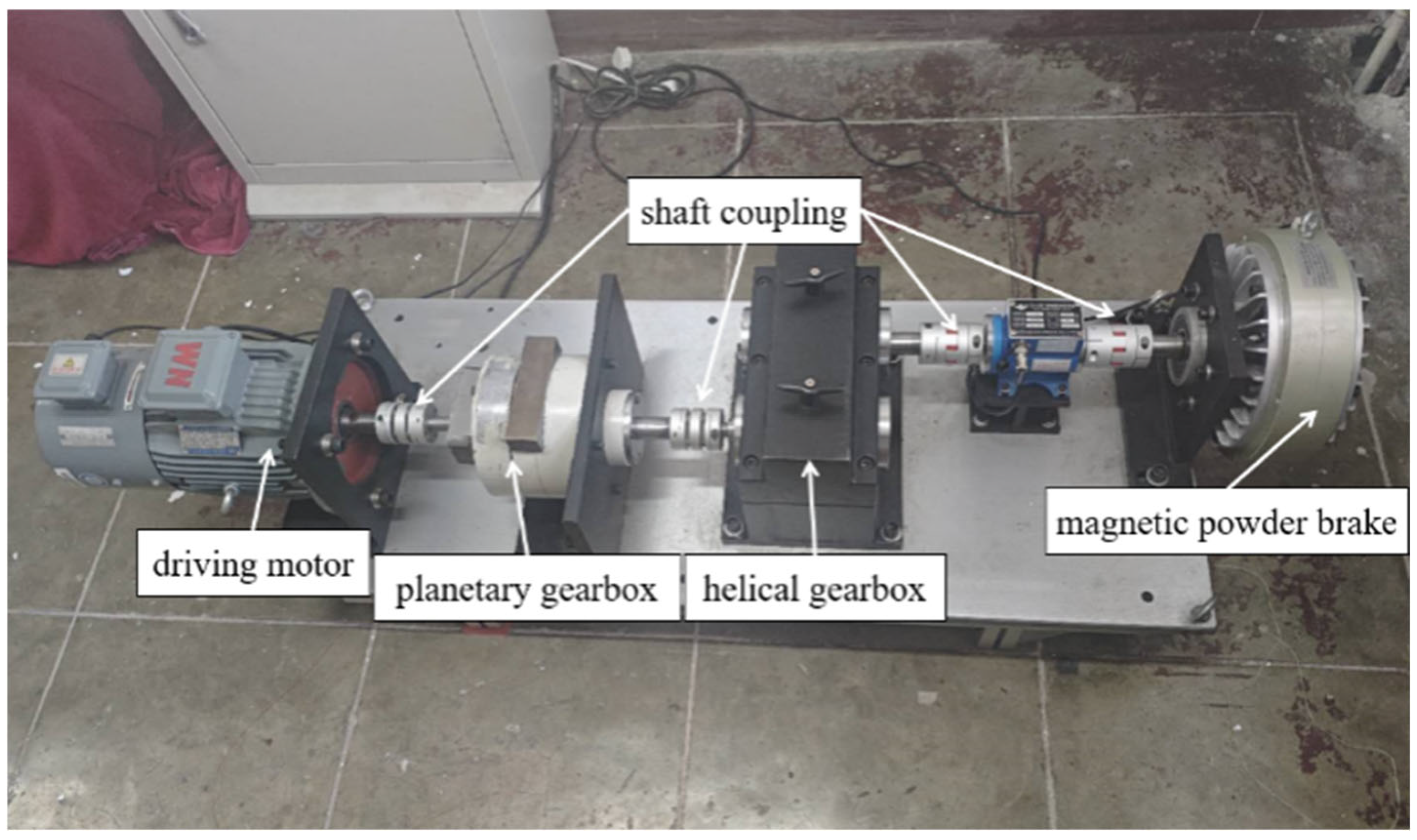
The test bench primarily consists of a variable-speed drive motor, multiple couplings, a planetary gearbox, a helical gearbox, and a magnetic powder brake. Its structure is illustrated in Figure 9. Six typical planetary gearbox states were selected from the laboratory dataset for experimental validation: healthy state, root crack in planetary gear teeth, pitting on planetary gear tooth surfaces, wear on planetary gear tooth surfaces, sun gear tooth fracture, and complete tooth breakage in the sun gear.

To simulate the actual operating load, the CZF-10 magnetic particle brake is used to increase the load. Its rated torque is 100 N·m, and the excitation current ranges from 0 to 2.5 A. When the gearbox operates at maximum speed, excessive load may cause the brake to sinter. Therefore, a load of 0 to 0.5 A is applied, which corresponds to an output torque of 0 to 20 N·m to simulate the actual working conditions.

In the actual operation of wind turbine gearboxes, the impact of complex working conditions—characterized by time-varying rotational speeds and variable loads caused by wind instability—on diagnostic results cannot be ignored. To better simulate the real operating conditions of wind turbine gearboxes, data collection for simulating variable working conditions was conducted in the laboratory. In addition to planetary gear faults, sun gear faults were also included; meanwhile, considering the noise interference from harsh environments, the data were divided into datasets as shown in

Table 7. Variable operating condition transfer learning dataset under strong noise.

Dataset	Number of Samples per Data Type	Operation Category	Operating Speed	Operating Load	Added Nosie Intensity
NUC-A	500	6	900 r/min	20 N m	−6, −4, −2, 0, 2
NUC-B	500	6	1500 r/min	0 N m	−6, −4, −2, 0, 2
NUC-C	500	6	time-varying rotational speed	10 N m	−6, −4, −2, 0, 2

. Dataset NUC-A represents the low-speed and heavy-load condition, Dataset NUC-B corresponds to the high-speed and light-load condition, while Dataset NUC-C stands for the condition with time-varying rotational speed and medium load.

To simulate the label-scarcity scenario in real environments where only a single type of data label is available, unsupervised fault diagnosis under variable conditions was performed across three datasets with different rotational speeds and loads. For each level of additional noise, the same experiment was repeated 5 times, and the average accuracy was taken as the result, as shown in

Table 8. Comparison of average accuracy of migration learning with different loss functions.

Migration Direction	Method	Average Accuracy
		−6 dB	−2 dB	0 dB	2 dB
A→B	CEL	75.89	77.58	76.34	78.48
A→B	CEL + 0.5 FBNM	83.42	84.68	85.82	85.31
A→B	CEL + 0.5 LMMD	92.78	97.57	98.38	98.78
A→B	CEL + 0.5 MS-LMMD	93.17	98.33	98.76	99.24
A→B	CEL + 0.5 MS-LMMD + 0.5 MSAF-CNN	94.67	99.41	99.76	100
A→C	CEL	73.45	75.86	75.22	77.28
A→C	CEL + 0.5 MSAF-CNN	80.24	82.43	82.84	83.12
A→C	CEL + 0.5 LMMD	89.67	94.57	97.24	98.45
A→C	CEL + 0.5 MS-LMMD	91.14	95.24	97.72	98.71
A→C	CEL + 0.5 MS-LMMD + 0.5 MSAF-CNN	94.78	98.11	99.07	99.81
B→A	CEL	80.57	84.24	84.92	85.24
B→A	CEL + 0.5 MSAF-CNN	85.89	86.33	87.04	88.48
B→A	CEL + 0.5 LMMD	95.33	96.82	97.67	98.33
B→A	CEL + 0.5 MS-LMMD	96.08	97.14	98.24	98.74
B→A	CEL + 0.5 MS-LMMD + 0.5 MSAF-CNN	98.41	99.45	99.93	100
B→C	CEL	77.65	80.33	79.84	80.67
B→C	CEL + 0.5 MSAF-CNN	81.47	82.67	81.59	83.55
B→C	CEL + 0.5 LMMD	93.14	95.74	97.24	98.12
B→C	CEL + 0.5 MS-LMMD	93.67	96.43	97.31	98.44
B→C	CEL + 0.5 MS-LMMD + 0.5 MSAF-CNN	94.33	97.24	97.85	99.24
C→A	CEL	84.75	83.52	84.17	85.24
C→A	CEL + 0.5 MSAF-CNN	89.65	89.54	90.42	88.67
C→A	CEL + 0.5 LMMD	97.47	98.33	99.85	100
C→A	CEL + 0.5 MS-LMMD	97.88	98.74	99.83	100
C→A	CEL + 0.5 MS-LMMD + 0.5 MSAF-CNN	98.35	99.94	100	100
C→B	CEL	82.25	83.52	82.17	84.28
C→B	CEL + 0.5 MSAF-CNN	87.62	87.54	86.92	88.16
C→B	CEL + 0.5 LMMD	95.87	97.67	98.84	99.06
C→B	CEL + 0.5 MS-LMMD	96.56	98.22	99.05	99.21
C→B	CEL + 0.5 MS-LMMD + 0.5 MSAF-CNN	97.88	99.34	100	100

.

It can be observed from the data table that the accuracy of all methods generally increases as the noise intensity decreases, which indicates the impact of noise on diagnostic accuracy.

Based on the transfer learning experimental results presented in Table 8, the proposed CEL + 0.5 MS-LMMD + 0.5 MSAF-CNN approach achieved optimal performance across all transfer directions and noise conditions. Particularly under the highly challenging −6 dB strong noise scenario, the diagnostic accuracy for each transfer task exceeded 94%, significantly outperforming other comparative methods. Progressive ablation analysis reveals that incorporating the LMMD loss yields a substantial improvement of approximately 15–20 percentage points, highlighting the critical role of subdomain alignment in cross-domain diagnosis. Further integration of MS-LMMD delivers an additional 0.5–1.5 percentage point gain in complex transfer tasks such as A→C and B→C, demonstrating the efficacy of multi-source local distribution alignment. The integration with MSAF-CNN enables the model to achieve near-100% accuracy in most scenarios, validating the synergistic enhancement effect of multi-source feature fusion and multi-source domain adaptation mechanisms. Moreover, as the signal-to-noise ratio improves from −6 dB to 2 dB, all methods gradually demonstrate enhanced performance. The proposed approach consistently maintains the highest accuracy and strongest robustness across various noise conditions, showcasing superior cross-operating-condition generalisation capability and engineering application value.

5. Concluding Remarks

This paper investigates the challenges of fault diagnosis for wind turbine planetary gearboxes under conditions of strong noise interference and sparse domain labelling. It proposes an intelligent diagnostic framework (MSFAF-CNN) that integrates multi-source vibration features with domain-adaptive strategies. By integrating channel and spatial attention mechanisms, it achieves dynamic weight allocation across multi-point vibration signals and complementary processing of heterogeneous features, significantly enhancing the model’s robustness and classification accuracy under low signal-to-noise ratio conditions. Furthermore, a multi-source local maximum mean difference (MS-LMMD) loss function is introduced. This innovatively performs independent subdomain distribution alignment for each measurement point prior to feature fusion, establishing a dual-layer domain adaptation constraint (‘measurement point fusion’). Finally, ablation experiments and cross-operating-condition transfer tasks designed using proprietary and publicly available planetary gearbox datasets validate the proposed method’s superior performance under strong noise and unknown operating conditions.

This paper organically integrates multi-source feature fusion with multi-source domain adaptation to construct a comprehensive fault diagnosis framework. It directly processes raw vibration signals, achieving high-precision fault diagnosis under noisy conditions (−4 dB to +4 dB). This provides an engineering-practical solution for intelligent equipment maintenance in complex industrial settings. Our approach demonstrated outstanding performance across the −4 dB to +4 dB test range, confirming its robustness in real-world industrial scenarios where such extreme noise levels are uncommon. Fault diagnosis under harsher conditions may necessitate integrated approaches combining advanced signal processing techniques, offering a promising avenue for future research. It should be noted that the validation work in this study is currently based on laboratory test benches and publicly available datasets. While these provide a solid foundation for evaluating the method, an inherent gap exists between laboratory environments and real-world wind farm operating conditions. The latter present greater challenges in terms of environmental noise complexity, operational variability, data quality, and the progressive and compound nature of faults.

References

1. Ahmad, H.; Cheng, W.; Xing, J.; Wang, W.; Du, S.; Li, L.; Zhang, R.; Chen, X.; Lu, J. Deep learning-based fault diagnosis of planetary gearbox: A systematic review. J. Manuf. Syst. 2024, 77, 730–745. [Google Scholar] [CrossRef]
2. Hu, M.T.; Wang, G.F.; Ma, K.L. Identification of wind turbine gearbox weak compound fault based on optimal empirical wavelet transform. Meas. Sci. Technol. 2023, 34, 108079. [Google Scholar] [CrossRef]
3. Xu, X.; Huang, X.; Bian, H.; Wu, J.; Liang, C.; Cong, F. Total process of fault diagnosis for wind turbine gearbox, from the perspective of combination with feature extraction and machine learning: A review. Energy AI 2024, 15, 100318. [Google Scholar] [CrossRef]
4. Tang, H.; Wang, H.; Li, C. Explainable fault diagnosis method based on statistical features for gearboxes. Eng. Appl. Artif. Intell. 2025, 148, 110503. [Google Scholar] [CrossRef]
5. Chen, S.Q.; Peng, Z.K.; Zhou, P. Review of Signal Decomposition Theory and Its Applications in Machine Fault Diagnosis. J. Mech. Eng. 2020, 56, 91–107. [Google Scholar]
6. Huang, N.E.; Shen, Z.; Long, S.R.; Wu, M.C.; Shih, H.H.; Zheng, Q.; Yen, N.-C.; Tung, C.C.; Liu, H.H. The empirical mode decomposition and the Hilbert spectrum for nonlinear and non-stationary time series analysis. Proc. R. Soc. Lond. A Math. Phys. Eng. Sci. 1998, 454, 903–995. [Google Scholar] [CrossRef]
7. Faris, E.; Amaral, J.T. Fault diagnosis and health management of bearings in rotating equipment based on vibration analysis—A review. J. Vibroeng. 2021, 24, 46–74. [Google Scholar]
8. Lei, Y.; Jia, F.; Kong, D.; Lin, J.; Xing, S. Opportunities and Challenges of Machinery Intelligent Fault Diagnosis in Big Data Era. J. Mech. Eng. 2018, 54, 94–104. [Google Scholar] [CrossRef]
9. Si, W.W.; Cen, J.; Wu, Y.B. Review of Research on Bearing Fault Diagnosis with Small Samples. Comput. Eng. Appl. 2023, 59, 45–56. [Google Scholar]
10. Li, X.; Ma, Z.; Yuan, Z.; Mu, T.; Du, G.; Liang, Y.; Liu, J. A review on convolutional neural network in rolling bearing fault diagnosis. Meas. Sci. Technol. 2024, 35, 2002. [Google Scholar] [CrossRef]
11. Zhang, W.; Peng, G.; Li, C.; Chen, Y.; Zhang, Z. A New Deep Learning Model for Fault Diagnosis with Good Anti-Noise and Domain Adaptation Ability on Raw Vibration Signals. Sensors 2017, 17, 425. [Google Scholar] [CrossRef] [PubMed]
12. Zhang, W.; Li, C.; Peng, G.; Chen, Y.; Zhang, Z. A deep convolutional neural network with new training methods for bearing fault di-agnosis under noisy environment and different working load. Mech. Syst. Signal Process. 2018, 100, 439–453. [Google Scholar] [CrossRef]
13. Zheng, B.; Huang, J.; Ma, X.; Zhang, X.; Zhang, Q. An unsupervised transfer learning method based on SOCNN and FBNN and its ap-plication on bearing fault diagnosis. Mech. Syst. Signal Process. 2024, 208, 111047. [Google Scholar] [CrossRef]
14. Huang, J.H.; Zheng, B.; Chen, G.Q. Fault diagnosis of bearing based on nuclear-norm maximization and unsupervised learning. Sci. Technol. Eng. 2023, 23, 4638–4646. [Google Scholar]
15. Ye, Z.; Yu, J. Multi-level features fusion network-based feature learning for machinery fault diagnosis. Appl. Soft Comput. J. 2022, 122, 108900. [Google Scholar] [CrossRef]
16. Huang, T.; Zhang, Q.; Tang, X.; Zhao, S.; Lu, X. A novel fault diagnosis method based on CNN and LSTM and its application in fault diagnosis for complex systems. Artif. Intell. Rev. 2021, 55, 1289–1315. [Google Scholar] [CrossRef]
17. He, K.; Zhang, X.; Ren, S.; Sun, J. Delving Deep into Rectifiers: Surpassing Human-Level Performance on ImageNet Classification. In Proceedings of the International Conference on Computer Vision, Las Condes, Chile, 11–18 December 2015. [Google Scholar]
18. Woo, S.; Park, J.; Lee, J.-Y.; Kweon, I.S. CBAM: Convolutional block attention module. arXiv 2018, arXiv:1807.06521. [Google Scholar] [CrossRef]
19. Iqbal, M.; Lee, C.K.M.; Keung, K.L. Fault diagnosis in rotating machines based on transfer learning: Literature review. Knowl.-Based Syst. 2024, 283, 111158. [Google Scholar]
20. Zhang, S.; Su, L.; Gu, J.; Li, K.; Zhou, L.; Pecht, M. Rotating machinery fault detection and diagnosis based on deep domain adaptation: A survey. Chin. J. Aeronaut. 2023, 36, 45–74. [Google Scholar] [CrossRef]
21. Liu, J. Bearing Fault Diagnosis Based on Incremental Transfer Learning and Ensemble Learning with Stochastic Configuration Network. Expert Syst. Appl. 2025, 290, 128398. [Google Scholar] [CrossRef]
22. Sun, K.; Huang, Z.; Mao, H.; Yin, A.; Li, X. Multiscale Margin Disparity Adversarial Network Transfer Learning for Fault Diagnosis. IEEE Trans. Instrum. Meas. 2023, 72, 3521712. [Google Scholar] [CrossRef]
23. Zhao, Y.-P.; Chen, Y.-B. Extreme learning machine based transfer learning for aero engine fault diagnosis. Aerosp. Sci. Technol. 2022, 121, 107311. [Google Scholar] [CrossRef]
24. Li, C.; Zhang, S.; Qin, Y.; Estupinan, E. A systematic review of deep transfer learning for machinery fault diagnosis. Neurocomputing 2020, 407, 121–135. [Google Scholar] [CrossRef]
25. Huang, M.; Yin, J.; Yan, S.; Xue, P. A fault diagnosis method of bearings based on deep transfer learning. Simul. Model. Pract. Theory 2023, 122, 102659. [Google Scholar] [CrossRef]
26. Li, X.; Yuan, P.; Su, K.; Li, D.; Xie, Z.; Kong, X. Innovative integration of multi-scale residual networks and MK-MMD for enhanced feature representation in fault diagnosis. Meas. Sci. Technol. 2024, 35, 6108. [Google Scholar] [CrossRef]
27. Chen, J.F. Research on Fault Diagnosis of Point Machine Plunger Pump Based on Multi-Source Feature Information Fusion. Ph.D. Thesis, North University of China, Taiyuan, China, 2024. [Google Scholar]
28. Zhu, Y.; Zhuang, F.; Wang, J.; Ke, G.; Chen, J.; Bian, J.; Xiong, H.; He, Q. Deep subdomain adaptation network for image classification. IEEE Trans. Neural Netw. Learn. Syst. 2021, 32, 1713–1722. [Google Scholar] [CrossRef]
29. Liu, D.D.; Cui, L.L.; Cheng, W.D. A review on deep learning in planetary gearbox health state recognition: Methods, appli-cations, and dataset publication. Meas. Sci. Technol. 2024, 35, 012002. [Google Scholar] [CrossRef]
Figure 1. Multi-source feature attention fusion convolutional neural network (MSFAF-CNN).
Applsci 15 12457 g001
Figure 2. CBAM attentional mechanisms.
Applsci 15 12457 g002
Figure 3. The application of PReLU in the convolutional module of each layer.
Applsci 15 12457 g003
Figure 4. Multi-scale convolutional structures for each channel.
Applsci 15 12457 g004
Figure 5. Data required for LMMD calculations at all levels.
Applsci 15 12457 g005
Figure 6. The dataset comprises vibration data collected from a planetary gearbox within a *wind turbine transmission system experimental apparatus.
Applsci 15 12457 g006
Figure 7. Confusion matrix of the two channels of SOCNN-CBAM at −4 dB are compared with those of MSFAF-CNN, as illustrated in Figure 7. (A) Employing the SOCNN-CBAM model in the x-direction (B) Employing the SOCNN-CBAM model in the y-direction (C) Employing the MSFAF-CNN model with XY-direction fusion.
Applsci 15 12457 g007
Figure 8. t-SNE dimensionality reduction.
Applsci 15 12457 g008
Figure 9. Gearbox failure simulation laboratory.
Applsci 15 12457 g009