Flow-Aware Trajectory Planning for Controlled-Altitude Balloons

Abstract

Autonomous high-altitude balloons are promising tools for studying dynamic environments. Their ability to navigate strong wind currents with minimal actuation makes them efficient options for scientific research. In fact, the flow in which these vehicles operate can both facilitate and restrict their ability to traverse the environment. Thus, to deploy the balloons effectively, motion planning becomes essential, requiring the consideration of both the environmental flows and the vehicle’s ability to maneuver through them. This paper proposes a probabilistic-based kinodynamic motion planner for an underactuated variable-altitude balloon navigating in flow-dominant environments. The proposed algorithm samples feasible control inputs rather than configurations to produce thrust commands that are within the physical actuation limits of the underactuated vehicle. In this paper, we consider both two-dimensional and three-dimensional vehicles with actuation in the vertical direction only. To test our method, simulations are shown for typical environments such as the double-gyre and the jet flows, and also for a more realistic environment based on Venus’ atmospheric wind flow.

1. Introduction

The deployment of autonomous vehicles in environments characterized by strong currents has emerged as a promising research area, offering a vast range of real-world applications. Within this context, lighter-than-air vehicles (LTAS) have gained traction in research and commercial domains [1,2]. Leveraging their buoyant properties, LTAs can remain aloft for extended periods without consuming excessive energy, promoting a broad scope of potential applications ranging from telecommunications to military surveillance and reconnaissance [3,4]. Aerostar, a company specializing in aerospace and defense solutions, has proposed using high-altitude balloons to facilitate cellular connectivity from the stratosphere, bridging communication gaps to denied or natural disaster-affected areas [5]. In the research realm, the implementation of various helium-filled balloons to support a recent NASA-sponsored study on Venus Aerial platforms is discussed in [6]. By exploiting the strong Venusian currents, researchers can use these platforms to study the atmospheric and volcanic activity on the planet, gaining key insight into the processes that shaped its climatic evolution.

Oceanographers have also proposed the use of similar platforms to perform crucial tasks such as ocean exploration and ice-shelf monitoring, gaining critical insights into previously inaccessible environments. The “IceNode” robots, for example, are tasked with collecting and returning data to the surface, allowing scientists to further understand the evolving environment [7]. The work presented in [8] underscores the potential of free-flying autonomous underwater vehicles (AUVs) to enhance subglacial exploration.

Whether underwater or in the air, motion planning is an important step in ensuring vehicles can perform their task. However, motion planning in such environments, especially those influenced by strong environmental flows, presents significant challenges. While the vehicle can leverage currents to traverse the environment, such currents often render various parts of the environment inaccessible or accessible at the cost of greater energy expenditure. From a motion planning perspective, traditional kinodynamic planning algorithms, such as [9,10], demonstrate the potential of probabilistic planning techniques to find suitable trajectories for systems such as hovercrafts and satellites but fail to account for environmental disturbances. Such methods rely on steering between sampled states by either solving the inverse kinematics problem or using a heuristic-based approach. For underactuated vehicles operating in flow-dominant environments, these strategies generate many invalid trajectories and can significantly increase computational time.

Some works have explicitly addressed the planning problem in environments with flow using traditional path-planning techniques. The work presented in [11,12] used A* in a two-dimensional environment for optimal trajectory planning in flows, considering both time and energy cost metrics. These papers provide further insight into how flows can be exploited to explore an environment and also illustrate how flow constraints can be integrated into path-planning algorithms. The work presented in [13] builds on these methods, focusing specifically on feasible trajectories in strong current fields. Langelaan’s group [14,15] presents tree-based trajectory planning by harnessing atmospheric energy for UAVs in complex wind fields. Branches of the search trees are deterministically computed based on a discrete set of allowable inputs, and the wind is considered during the tree expansion. Different from the work presented in our paper, these previous methods tackle graph/tree construction by discretization rather than using probabilistic-based sampling methods.

Sampling-based planning was used before by our group for navigation in windy environments [16,17]. Among the proposed methods, the FlowFMT* algorithm presented in [17] offers robust navigation in strong currents using a fast marching tree approach, which is an asymptotically optimal method. The paper defines wind-based feasibility regions, which are used to determine feasible connections between nodes of the search tree. The same feasibility regions were used in [18] to check the validity of paths generated by genetic algorithms. These works assume full actuation capabilities, a luxury not afforded by certain vehicles, such as the balloons considered in this paper, which can only control their altitude through buoyancy adjustments.

Most of the limited research on controlled-altitude balloons focuses on station keeping [19,20,21]. In contrast, the work presented in [22] introduces a probabilistic approach using a Markov decision process (MDP) to optimize traversal times of controlled-altitude balloons by selecting favorable altitudes. The paper builds upon a previous work of the same group that also uses MDP to guide buoyancy-controlled vehicles in uncertain under-ice ocean flows [23]. A recent study presented in [24] addresses the challenge of navigating balloons between two three-dimensional positions in environments with wind. Their control framework is based on reinforcement learning, which has previously been applied for station keeping [19]. The authors report interesting results from experiments conducted with real-world balloons in both indoor and outdoor settings. While the problem formulation closely resembles that of the present paper, their approach is controller-based, whereas this paper proposes a planner-based methodology. By employing a planner instead of a controller, our method enables the vehicle to avoid prohibited regions within the space, which are not considered by any of the previous research in the area.

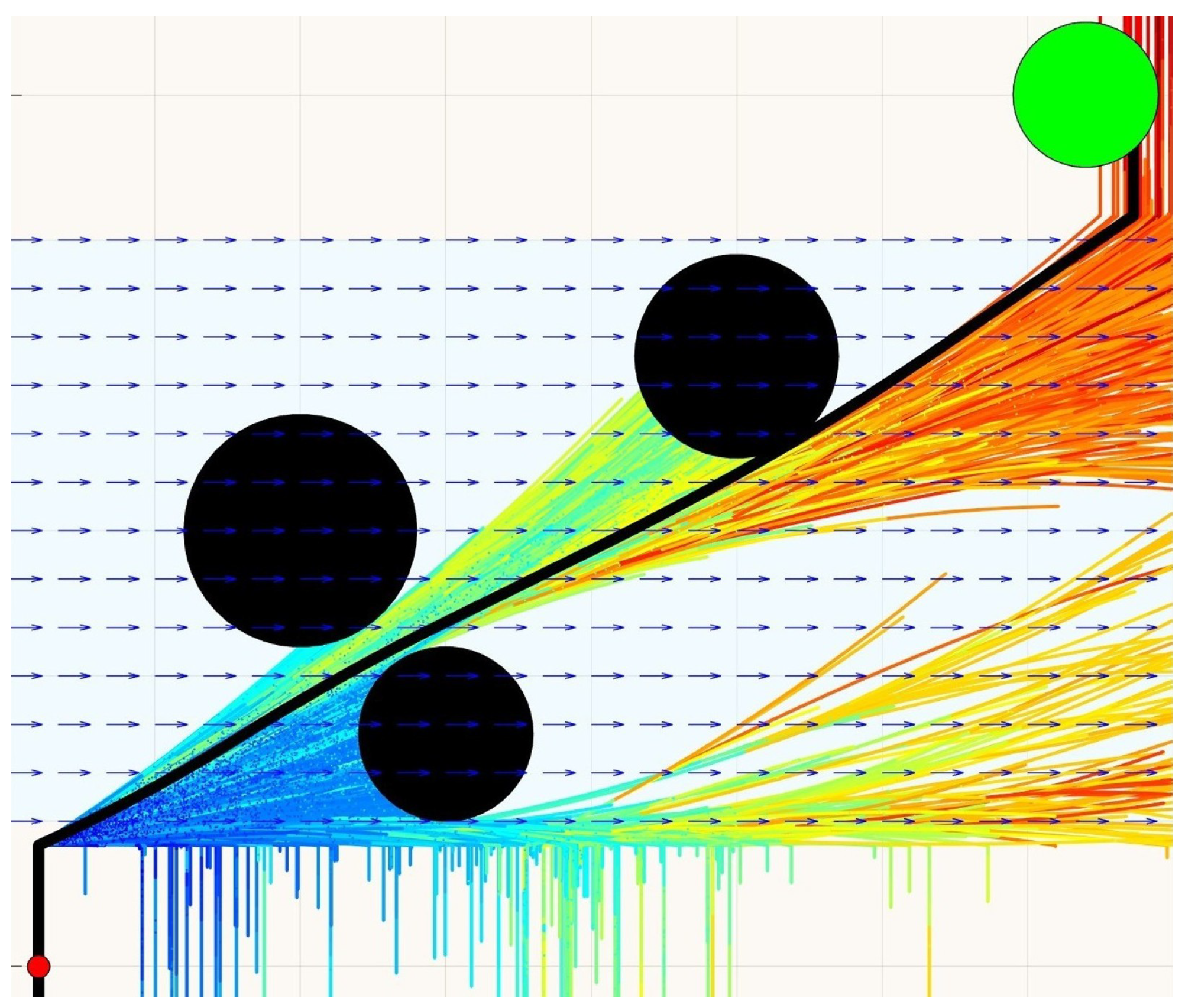
The objective of this paper is to present a motion planning approach for underactuated vehicles navigating flows in the presence of obstacles and/or no-fly zones. Figure 1 illustrates our approach, which creates a tree of feasible trajectories that safely guide the vehicle to any reachable position in the environment. The vehicle considered in our paper is inspired by high-altitude balloons, which can control their altitude by altering their buoyancy. Since the change in altitude is the only controlled input of the balloon, it mostly drifts with the wind and can only reach its goal if it correctly decides when to go up or down, so it can drift in the desired direction. Our proposed motion planner employs a sampling-based approach to determine both the vehicle’s control input and the duration for which it should be applied. The method samples directly in the control space, effectively creating a kinodynamic motion planner that satisfies the dynamic constraints of the vehicle. After control inputs are sampled, positions are obtained through model integration. Sampling in the control space inherently addresses the challenge of unrealistic sample generation, as the algorithm only produces feasible samples that do not violate physical actuation limitations. Furthermore, actuation commands are directly mapped to nodes in the graph, simplifying the execution of planned trajectories.

The remainder of this paper is organized as follows. Section 2 addresses the problem being solved. Section 3 describes the proposed method, and Section 4 provides the experimental results. Lastly, conclusions and suggestions for future work are discussed in Section 5.

2. Problem Definition

2.1. Environment

In this paper, we assume a vehicle operating in a 3D environment $\mathcal{W}\subset {\mathbb{R}}^3$ in the presence of a flow field. The velocity of the flow at any point in the space $\overrightarrow{x}={[x,y,z]}^T\in \mathcal{W}$ is defined as ${\overrightarrow{v}}_c={[v_{c_x},v_{c_y},v_{c_z}]}^T\in {\mathbb{R}}^3$. We consider that certain regions of the environment cannot be traversed by the vehicle and must be avoided. These regions may or may not change the behavior of the flow. For simplicity and without loss of generality, in this work, such regions are defined as spheres by $O_i=\{(x,y,z)\in \mathcal{W}\mid {(x-c_{x_i})}^2+{(y-c_{y_i})}^2+{(z-c_{z_i})}^2\le r_i^2\}$ where ${[c_{x_i},c_{y_i},c_{z_i}]}^T$ represents the center of the region and $r_i$ represents its radius.

2.2. Vehicle

We consider an underactuated vehicle (balloon) operating in a flow-dominated environment. The vehicle is assumed to be small relative to the scale of the environment and is modeled as a point mass. As such, its size, shape, and orientation are neglected. The vehicle can only produce vertical acceleration and is influenced by the environmental flow field. We define the control input $u_z$ as a discrete command issued to the vehicle, corresponding to one of three action modes: pump, vent, or idle. We assume that the balloon carries a helium tank, so the action pump means that helium is removed from the balloon’s envelope and stored in the tank (the balloon should go down). Vent, on the other hand, means that helium is released to the envelope (the balloon goes up), while in idle, no transfer of helium happens. Pump and vent actions are discretized in four levels (25, 50, 75, and $100\%$), corresponding to the volume of helium being removed or released from the balloon per time unit. Therefore, nine discrete inputs are available for the balloon: four related to the pump action, four related to the vent action, and one representing the idle state. We model each input as producing a constant vertical acceleration $a_{r_z}$. The magnitudes of $a_{r_z}$ are bounded by environment-specific limits that ensure the vehicle remains underactuated. In practice, these inputs would yield accelerations governed by the system’s full dynamics [25], but we assume idealized, constant effects to enable efficient sampling and planning.

The relative velocity of the vehicle with respect to the flow is denoted as ${\overrightarrow{v}}_r={[v_{r_x},v_{r_y},v_{r_z}]}^T$. In this underactuated model, we assume $v_{r_x}=v_{r_y}=0$ since only the vertical component $v_{r_z}$ is actuated. To simulate the vehicle’s motion, this velocity component is obtained by numerically integrating the vertical acceleration $a_{r_z}$ over a small time interval $dt$. To ensure physical realism, the relative vertical velocity is bounded such that $v_{r_z}\in [-v_{r_z}^{\max },v_{r_z}^{\max }]$. Once this limit is reached, the commanded acceleration is set to zero, preventing further speed increases. The global velocity of the vehicle is then given by:

$${\overrightarrow{v}}_g={\overrightarrow{v}}_r+{\overrightarrow{v}}_c.$$

(1)

2.3. Problem Statement

This work addresses the problem of finding feasible trajectories for the vehicle defined in the previous subsection from a given initial state ${\overrightarrow{x}}_0={[x_0,y_0,z_0]}^T$ at time $t=0$ to a reachable final position ${\overrightarrow{x}}_f={[x_f,y_f,z_f]}^T$ at time $t=t_f$, which belongs to a goal region defined as a sphere by $\mathcal{G}=\{(x,y,z)\in \mathcal{W}\mid {(x-c_{x_g})}^2+{(y-c_{y_g})}^2+{(z-c_{z_g})}^2\le r_{\mathrm{goal}}^2\}$, where ${\overrightarrow{x}}_{\mathrm{goal}}={[c_{x_g},c_{y_g},c_{z_g}]}^T$ is the center of the goal and $r_{\mathrm{goal}}$ is the goal radius. The planned trajectories must avoid all prohibited regions $O_i$. To enable trajectory execution, the solution must provide a time-parameterized sequence of control inputs, $u_z$, as discussed before.

3. Methodology

This section presents the proposed trajectory planning algorithm, which is inspired by the Rapidly-exploring Random Tree (RRT) framework [26], but fundamentally differs from it by incorporating control-space sampling in environments characterized by time-invariant flow fields.

3.1. Flow-Aware Trajectory Planning

The proposed method utilizes a sampling strategy that operates directly in the control space. Specifically, instead of sampling random positions or velocities, the planner samples discrete control inputs. Each input is mapped to a vertical acceleration, which is used to forward integrate the vehicle’s motion for a given interval of time. After the motion is integrated, a new node for a search tree is created. This approach ensures that all generated trajectories are dynamically feasible, flow-aware, and naturally respect the reachability constraints imposed by the environment. 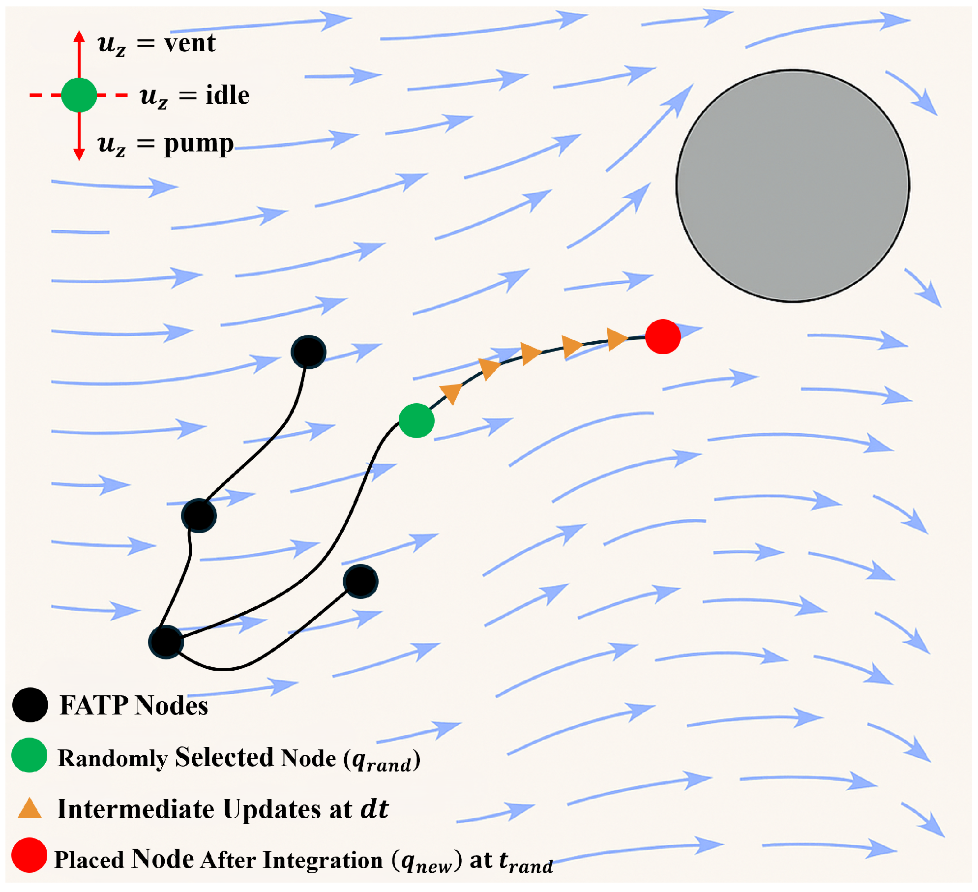Because the sampling process inherently considers the effects of the flow, it eliminates the need for artificial bounding of sampled positions or post-processing to remove invalid or unreachable trajectories [18]. This strategy is particularly well-suited for underactuated systems, where flow velocities dictate passive movement directions, and control authority is restricted to a single dimension. Algorithm 1 outlines the structure of the proposed trajectory planner, which is illustrated in Figure 2. While it is inspired by the standard RRT framework [26], the key distinction lies in the sampling phase (line 3), where our method uses a control-space sampling strategy coupled with forward integration to generate dynamically feasible trajectories.

Algorithm 1. Flow-Aware Probabilistic Trajectory Planner (FATP)

1: $V\leftarrow \left\{x_0\right\};E\leftarrow \varnothing$  2: for $i=1,\dots ,n$ do  3:       $(q_{\mathrm{new}},q_{\mathrm{nearest}},\mathtt{vehicle},\mathtt{cost})\leftarrow \mathtt{FlowAwareControlSampling}\left(G\right)$  4:       $V\leftarrow V\cup \left\{q_{\mathrm{new}}\right\}$  5:       $E\leftarrow E\cup \left\{(q_{\mathrm{nearest}},q_{\mathrm{new}})\right\}$  6:       if $\parallel q_{\mathrm{new}}-x_{\mathrm{goal}}\parallel \le r_{\mathrm{goal}}$ then  7:           break  8:       end if  9: end for 10: return $G=(V,E)$

The algorithm begins by initializing the vertex set with the start position (root of the tree) and an empty edge set (line 1). For each iteration up to the desired number of samples n (line 2), the planner calls the FlowAwareControlSampling function (line 3), which returns a new vertex $q_{\mathrm{new}}$, its parent $q_{\mathrm{nearest}}$ on the current tree, a vehicle structure containing the control input $u_z$, applied acceleration $a_{r_z}$, and resulting global vertical velocity $v_{g_z}$, as well as a cost structure containing the travel time $t_{\mathrm{new}}$, distance $d_{\mathrm{new}}$, and an energy/work metric. The vehicle structure contains information necessary for forward integration in subsequent iterations, while the cost structure supports trajectory querying and performance evaluation. The new vertex is added to the tree (line 4), and the edge from its parent is recorded (line 5). An optional break condition (line 6) checks if the search tree entered the goal region. To allow more than one trajectory leading to the goal region, this condition can be removed at the expense of more processing time. The algorithm returns the final tree $G=(V,E)$ (line 10) from which trajectories can be extracted.

3.2. Control Space Sampling

Algorithm 2 outlines the FlowAwareControlSampling function, which generates new feasible nodes through forward integration. The algorithm repeats until a valid sample is produced (line 1). It begins by selecting a random node from the current graph (line 2), maintaining the probabilistic nature of sampling-based motion planning. The initial vertical velocity $v_{g_z}$ needed to ensure continuity between segments is inherited from the parent node (line 3). Rather than sampling a position or velocity directly, the algorithm samples a discrete control input $u_z$, representing a throttling state corresponding to one of several action modes (e.g., pump, vent, or idle) (line 4). Each input maps to a fixed acceleration $a_{r_z}$, expressed as a percentage of a predefined maximum acceleration (line 5).

Algorithm 2. FlowAwareControlSampling(G)

1: while True do  2:       $q_{\mathrm{nearest}}\leftarrow \mathtt{RandomNode}\left(G\right)$  3:       $v_{g_z}\leftarrow \mathtt{GetParentVerticalVelocity}\left(q_{\mathrm{nearest}}\right)$  4:       $u_z\leftarrow \mathtt{RandomControlState}\left(\right)$  5:       $a_{r_z}\leftarrow \mathtt{AccelerationFromControl}\left(u_z\right)$  6:       $t_{\mathrm{rand}}\leftarrow \mathtt{rand}(t_{min},t_{max})$  7:       $dt\leftarrow t_{min}$  8:       $q_{\mathrm{new}}\leftarrow q_{\mathrm{nearest}}$  9:       $t_{\mathrm{new}}\leftarrow 0$,    $d_{\mathrm{new}}\leftarrow 0$ 10:     while $t_{\mathrm{new}}<t_{\mathrm{rand}}$ do 11:           ${\overrightarrow{v}}_{\mathrm{c}}\leftarrow \mathtt{GetFlowVelocity}\left(q_{\mathrm{new}}\right)$ 12:           $v_{r_z}\leftarrow \mathtt{RelativeVerticalVelocity}\left(q_{\mathrm{new}}\right)$ 13:           $v_{r_z}\leftarrow v_{r_z}+a_{r_z}·dt$ 14:           if $|v_{r_z}|>v_{r_z,max}$ then 15:                $a_{r_z}\leftarrow 0$ 16:           end if 17:           ${\overrightarrow{v}}_{\mathrm{g}}\leftarrow [v_{{\mathrm{c}}_x},v_{{\mathrm{c}}_y},v_{{\mathrm{c}}_z}+v_{r_z}]$ 18:           $q_{\mathrm{next}}\leftarrow q_{\mathrm{new}}+{\overrightarrow{v}}_{\mathrm{g}}·dt$ 19:           $d_{\mathrm{new}}\leftarrow d_{\mathrm{new}}+\parallel {\overrightarrow{v}}_{\mathrm{g}}·dt\parallel$ 20:           $t_{\mathrm{new}}\leftarrow t_{\mathrm{new}}+dt$ 21:           $w_{\mathrm{new}}\leftarrow \left|a_{r_z}\right|·d_{\mathrm{new}}$ 22:           if $\neg \mathtt{isFree}\left(q_{\mathrm{next}}\right)$ or $q_{\mathrm{next}}\notin \mathtt{bounds}$ then 23:                 if $t_{\mathrm{new}}=0$ then 24:                     break 25:                 else 26:                       return $q_{\mathrm{new}},q_{\mathrm{nearest}},\mathtt{vehicle}=(u_z,a_{r_z},v_{g_z}),\mathtt{cost}=(t_{\mathrm{new}},d_{\mathrm{new}},w_{\mathrm{new}})$ 27:                 end if 28:           end if 29:           $q_{\mathrm{new}}\leftarrow q_{\mathrm{next}}$ 30:     end while 31:     return $q_{\mathrm{new}},q_{\mathrm{nearest}},\mathtt{vehicle}=(u_z,a_{r_z},v_{g_z}),\mathtt{cost}=(t_{\mathrm{new}},d_{\mathrm{new}},w_{\mathrm{new}})$ 32: end while

A random integration duration $t_{\mathrm{rand}}$ is drawn from a user-defined interval $[t_{min},t_{max}]$ (line 6), and a fixed integration step size $dt=t_{min}$ is used. The main loop (starting in line 10) forward integrates the vehicle’s state by computing the global velocity ${\overrightarrow{v}}_g$ using (1) and ensuring the algorithm does not produce unrealistic vehicle velocities (lines 12–16). At each step, the vehicle’s position (line 18) is updated using:

$$q_{\mathrm{new}}=q_{\mathrm{rand}}+\sum _{i=1}^N{\overrightarrow{v}}_g^{\left(i\right)}·dt,$$

(2)

where ${\overrightarrow{v}}_g^{\left(i\right)}=[v_{c_x}^{\left(i\right)},v_{c_y}^{\left(i\right)},v_{c_z}^{\left(i\right)}+v_{r_z}^{\left(i\right)}]$ is the global velocity at integration step i, and $dt$ is the time increment. The number of integration steps N is given by $N=⌊{\displaystyle \frac{t_{\mathrm{rand}}}{dt}}⌋$. The cumulative time, distance, and energy are also incremented (lines 19–21). The distance $d_{\mathrm{new}}$ is computed as the path integral of the global velocity, and the energy $w_{\mathrm{new}}=\left|a_{r_z}\right|·d_{\mathrm{new}}$ is computed to approximate actuation effort.

If the propagated state remains within bounds and avoids collision, it is accepted and integrated further. If a collision is detected at the first step, the loop restarts with a new random control input (lines 23–24). If a collision occurs after progress has been made, the last valid state is returned (line 26). Upon successful completion, the function returns the updated node $q_{\mathrm{new}}$, its parent $q_{\mathrm{nearest}}$, and the two structure outputs vehicle and cost. These values are used in Algorithm 1 to construct dynamically feasible, flow-consistent trajectories.

Once Algorithm 1 returns the tree represented by G, a trajectory from the start node to any node in the tree can be recovered by following the back-pointers (i.e., parent nodes) from the goal node to the start node. After the trajectory is constructed, the control and cost metrics stored at each node can be used by the vehicle to execute the trajectory and evaluate performance.

Although the proposed algorithm does not guarantee optimal trajectories, it supports efficient retrieval of low-cost trajectories by querying the constructed tree. After identifying nodes within the goal region, the best trajectory can be selected based on a user-defined cost metric, which can be either time, distance, or energy saved in each node.

3.3. Analysis

The proposed Flow-Aware Trajectory Planning (FATP) algorithm is not optimal, as it does not guarantee convergence to the best-cost trajectory. The algorithm is, however, probabilistically complete, meaning that a solution will be found with high probability as the number of samples increases. The time for finding the trajectory is influenced by tunable parameters such as the maximum integration time $t_{\max }$, which plays a role analogous to the steering step in the traditional RRT. While prior work has shown that directly sampling control inputs can bias tree growth toward already explored regions [9], this bias is mitigated in flow-dominant environments where exploration is shaped primarily by the underlying flow field and integration dynamics.

To prove that the FATP algorithm is probabilistically complete, assume the existence of a feasible trajectory $\tau \left(t\right)$. Further, assume that $\tau \left(t\right)$ is covered by a sequence of intersecting balls $B_1,B_2,\dots ,B_k$, such that $B_1$ contains the starting position and $B_k$ intersects the goal region. The radius of these balls is chosen to be less than or equal to the clearance of the trajectory from the obstacles to ensure that each ball lies entirely within the free space. Since the trajectory exists, each ball may be displaced vertically and/or horizontally relative to the previous one. However, the horizontal displacement must always be in the positive direction of the flow, as the vehicle cannot move against it. Thus, for each pair $(B_{i-1},B_i)$, there exists a control input $u_z$ and an integration time $t_{\mathrm{rand}}$ that guides the vehicle from $B_{i-1}$ to $B_i$. At each interaction of FATP, a node from the tree is randomly selected. Since the starting position lies within $B_1$, and all subsequent nodes are generated by forward integration from existing ones, the probability that the selected node lies within one of the balls is non-zero. Additionally, because control inputs and integration times are sampled randomly, the probability of generating a valid pair that guides the vehicle to the next ball is also non-zero. Moreover, the probability of consistently selecting nodes outside the balls and failing to generate all valid control inputs and integration times necessary to reach $B_i$ from $B_{i-1}$ decreases exponentially with the number of samples. Therefore, the probability of reaching the goal region starting from $B_1$ approaches 1 as the number of samples increases, indicating that FATP is probabilistically complete.

The time complexity of the proposed method is favorable compared to traditional kinodynamic planners, as the algorithm avoids costly nearest-neighbor searches by growing the tree through random node selection rather than proximity-based expansion. The cost of selecting a node of the tree can be as fast as $O\left(1\right)$, if the nodes are stored in an array. Since all other functions invoked by Algorithm 2, including the GetFlowVelocity function, which may retrieve the flow from a lookup table, do not depend on the number of samples, they are all $O\left(1\right)$ time. Therefore, the complexity of FATP is $O\left(n\right)$, where n is the number of samples. Similar to RRT, the space complexity is $O\left(n\right)$, since the algorithm stores the parent, cost, and control input for each node of the tree.

4. Experimental Results

This section presents the evaluation of the proposed trajectory planning algorithm in a variety of flow environments. The environments are categorized into three types: jet flow, gyre flow, and Venusian atmospheric flow. For each type, we analyze the algorithm’s performance in two and three dimensions, except the Venusian flow, which is considered only in three dimensions. Our results focus on the feasibility of generated trajectories, adaptation to local flow dynamics, and the influence of actuation constraints on reachable regions. Plots and metrics are provided to illustrate tree growth, trajectory diversity, and environmental interactions. Where applicable, the tree is colored by cumulative cost from the initial configuration, providing visual insight into the progression of the graph structure. Simulations were performed using MATLAB R2024b on an Intel® Core™ i7-7820X CPU running at 3.6 GHz, featuring 8 cores and 64 GB of RAM.

4.1. Jet Flow Environment

The jet flow environment is characterized by regions of high-velocity magnitude and sharp flow boundaries. Such flow profiles are often used to model atmospheric jets, propulsion systems, high-pressure nozzles, and various pneumatic or hydraulic systems. These environments serve as ideal testbeds for evaluating motion planners under strong directional currents [27].

The three-dimensional jet flow used in this work is defined as:

$${\overrightarrow{v}}_c(x,y,z)=\left\{\begin{array}{cc}{[20.0,0.0,0.0]}^T\mathrm{m}/\mathrm{s},\hfill & \mathrm{if}y,z\in [40,60]\mathrm{m}\hfill \\ {[0.0,0.0,0.0]}^T\mathrm{m}/\mathrm{s},\hfill & \mathrm{otherwise}.\hfill \end{array}\right.$$

(3)

This flow represents a horizontal jet directed along the positive x-axis, with nonzero velocity confined to the region $40\le y\le 60$ and $40\le z\le 60$. Outside this jet region, the flow is quiescent. The simulation domain was defined as $\mathcal{W}=[0,100]\mathrm{m}\times [30,70]\mathrm{m}\times [30,70]\mathrm{m}$ to restrict the vehicle’s motion to a corridor surrounding the jet. The relative vertical velocity of the vehicle was limited to $v_{r_z}=10\mathrm{m}/\mathrm{s}$ and its acceleration to $a_{r_z}=20\mathrm{m}/{\mathrm{s}}^2$. Unless we say otherwise, the integration step was set to $dt=t_{\min }=1$ms and the maximum integration time to $t_{\max }=1$s.

4.1.1. 2D Jet Flow

The two-dimensional jet flow considered in this work is a simplified representation of the full 3D flow described in (3) when the movement is restricted to the plane $z=0$. In this case, we assume that the vehicle’s actuation is constrained to the y-direction.

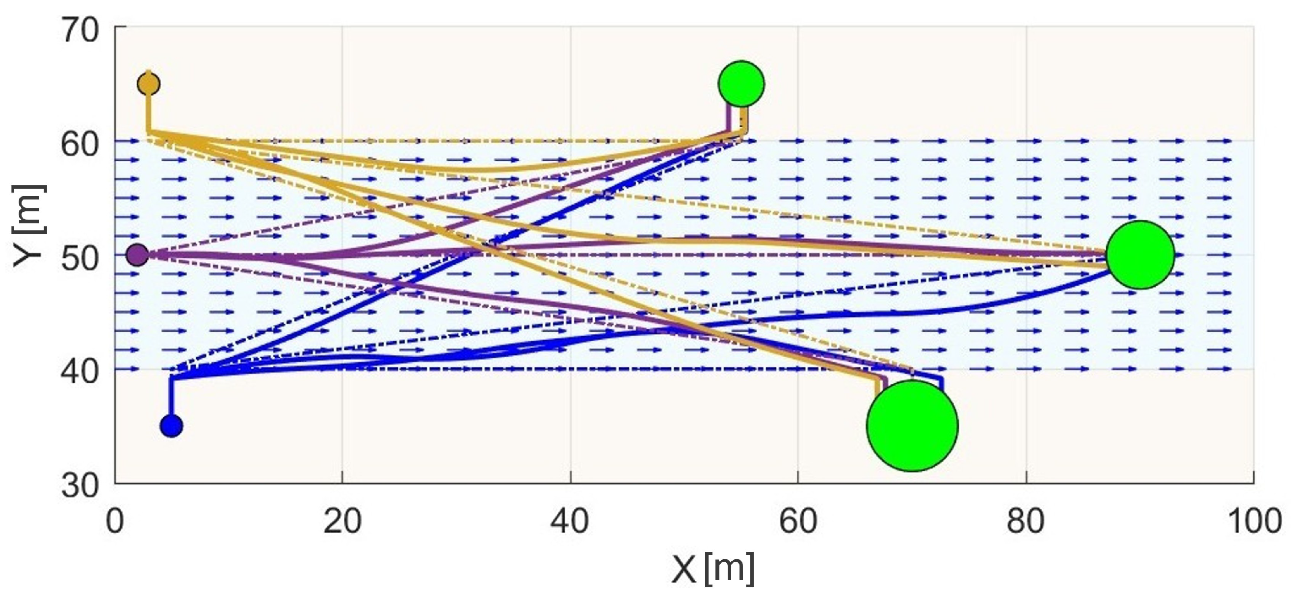
To benchmark the planner’s performance, an analytical minimum-distance trajectory is derived for each goal region, assuming a vehicle that is underactuated and only capable of vertical control. The resulting trajectories consist of piecewise segments aligned with the vehicle’s actuation limits and the structure of the jet. Figure 3 compares the analytically optimal distance-minimizing trajectories from a common start location to three distinct goal regions in the 2D jet flow environment with the trajectories found by our algorithm. For the minimum-distance solution, each trajectory is designed to minimize vertical and horizontal travel by exploiting the structure of the jet flow. When the vehicle starts outside the jet, it first performs a vertical maneuver to enter the flow region. Once within the jet, it passively drifts by maintaining a constant vertical velocity, allowing the horizontal component of motion to be governed entirely by the environmental flow. If the goal lies outside the jet, a final vertical maneuver is performed to exit the flow and reach the target altitude. When the vehicle starts within the jet and the goal also lies within or along its path, the vehicle may bypass any initial vertical actuation and instead drift directly to the goal.

Table 1. Comparison of analytical minimum-distance and FATP (Flow-Aware Trajectory Planning) costs for various start and goal configurations. All values are in meters.

Start Position	Goal Position	Analytical Distance (m)	FATP Distance (m)
$[5,35]$	$[55,65]$	$63.85$	$64.59$
	$[70,35]$	$75.00$	$77.80$
	$[90,50]$	$87.59$	$91.28$
$[2,50]$	$[55,65]$	$58.94$	$60.54$
	$[70,35]$	$73.73$	$74.97$
	$[90,50]$	$88.00$	$88.56$
$[3,65]$	$[55,65]$	$62.00$	$63.96$
	$[70,35]$	$79.92$	$81.77$
	$[90,50]$	$92.57$	$93.30$

quantifies the distance cost associated with each analytically derived trajectory and compares it to the result produced by the proposed Flow-Aware Trajectory Planning (FATP) method. The analytical costs represent theoretical lower bounds assuming ideal control execution, while the FATP costs reflect sampled trajectories generated during tree construction. While the FATP-generated trajectories are not guaranteed to be optimal, they still yield reasonable and feasible trajectories in flow-dominant environments.

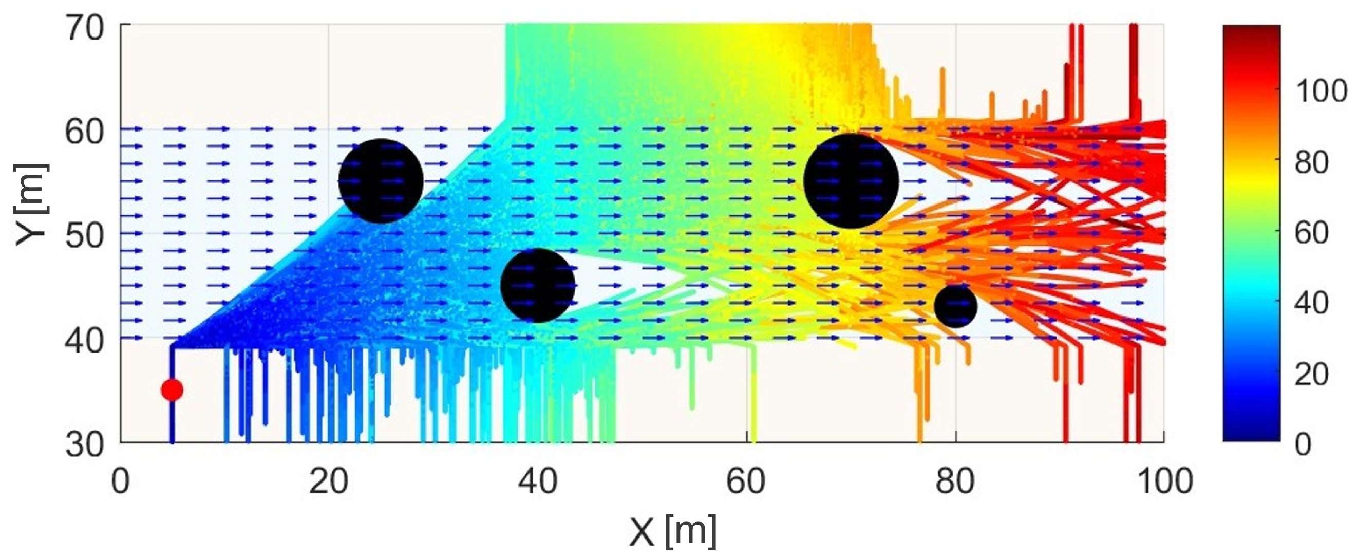
Figure 4 illustrates the impact of an obstacle-rich environment on planning and highlights the computational efficiency of the proposed method in such environments. In the obstacle-rich environment, the runtime to create a tree with $\mathrm{30,000}$ samples was $63.483$ s, which is comparable to the obstacle-free case (tree not shown here), at $55.853$ s. This result highlights that the presence of obstacles does not significantly affect computation time, as obstacle avoidance is performed during forward integration rather than through explicit collision checks. It is important to mention that computing analytical solutions for such obstacle-rich environments is very difficult, thus justifying the use of the proposed algorithm, even for simple flow environments. Computational time also benefits from the planner not requiring a separate nearest-neighbor search or steering function as seen in traditional probabilistic planners. Finally, notice in Figure 4 that, due to the vehicle’s underactuated nature, certain regions of the environment are unreachable, particularly those requiring lateral movement against the flow. This limitation is reflected in the absence of tree growth in those regions.

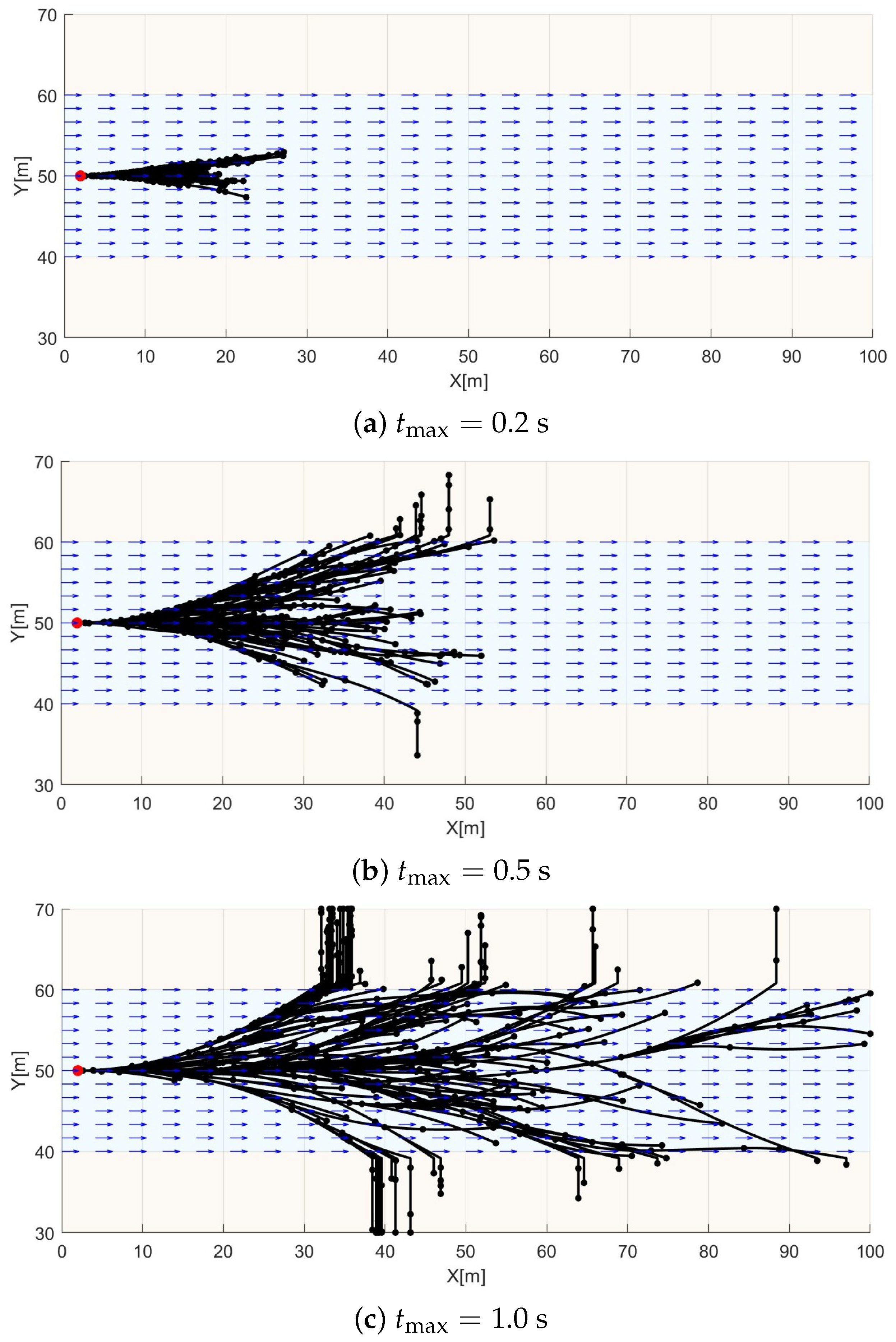
We also investigated the effect of one of the most important parameters of the proposed method, which is the maximum integration time, $t_{\max }$. For this, we ran the FATP algorithm with three different values of $t_{\max }$, but kept the number of samples and the integration step constant. The search trees in Figure 5 show that larger values of $t_{\max }$ allow for more exploration of the environment, while the smaller values yield denser trees. It is then expected that a small $t_{\max }$ gives more trajectory options towards the goal. On the other hand, the first trajectory can be found with a smaller number of samples if a larger $t_{\max }$ is used. However, a small number of samples does not necessarily mean a faster plan, since a larger $t_{\max }$ corresponds to larger integration times, which can be very slow depending on the vehicle’s model. For the simple model used in this paper, the computation times for Figure 5a–c were, respectively, $0.8768$, $0.9339$, and $1.8887$ s. Thus $t_{\max }$ is chosen to balance global exploration with local precision and to manage the trade-off between the number of nodes required to find a solution and the processing time.

4.1.2. 3D Jet Flow

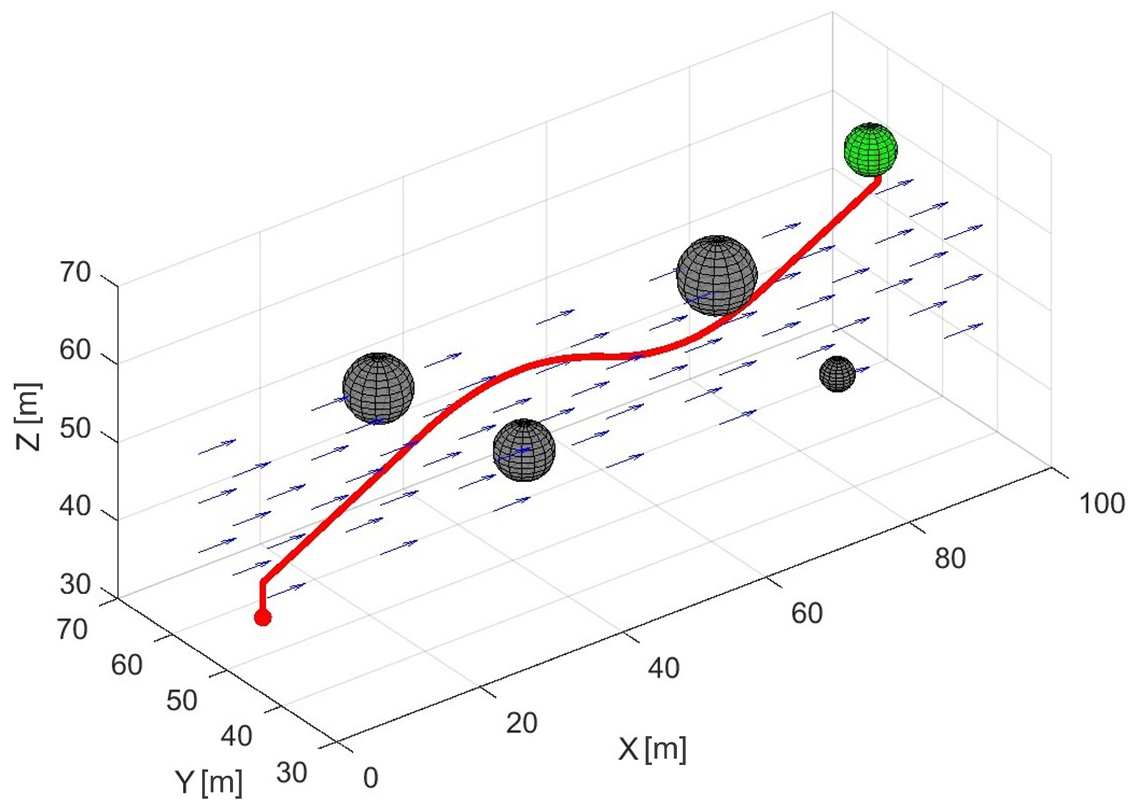
Figure 6 presents results for the 3D jet flow environment for a starting configuration of $(x_0,y_0,z_0)=(5,50,35)$ m and a goal region centered at $(x_g,y_g,z_g)=(90,50,65)$ m. The tree construction was terminated with $\mathrm{14,872}$ samples when the goal was reached. The total computational time was $37.26$ s. Despite the increased dimensionality, the planner remained efficient and successfully produced a trajectory that avoids obstacles while exploiting the structure of the jet corridor.

4.2. Gyre Flow Environment

The gyre flow environment used in this work is derived from the standard double-gyre model [12], which describes a time-invariant flow commonly used to benchmark flow-aware planning algorithms. The three-dimensional formulation of the velocity field is given by:

$${\overrightarrow{v}}_c(x,y,z)=\left\{\begin{array}{c}-\pi Asin\left({\displaystyle \frac{\pi x}{s}}\right)cos\left({\displaystyle \frac{\pi y}{s}}\right)cos\left({\displaystyle \frac{\pi z}{s}}\right)\mathrm{m}/\mathrm{s},\hfill \\ \pi Acos\left({\displaystyle \frac{\pi x}{s}}\right)sin\left({\displaystyle \frac{\pi y}{s}}\right)cos\left({\displaystyle \frac{\pi z}{s}}\right)\mathrm{m}/\mathrm{s},\hfill \\ \pi Asin\left({\displaystyle \frac{\pi z}{s}}\right)\mathrm{m}/\mathrm{s},\hfill \end{array}\right.$$

(4)

where A is the amplitude of the flow, and s is the spatial scaling factor. In alignment with [17], the parameters were selected as $A=2$ and $s=1$. The vehicle’s maximum velocity relative to the flow was chosen such that $v_{r_z}=5\mathrm{m}/\mathrm{s}$, limiting its ability to overcome strong opposing flows and preventing traversal through all regions of the environment. The vehicle’s maximum vertical acceleration was set to $a_{r_z}=20\mathrm{m}/{\mathrm{s}}^2$.

4.2.1. Two-Dimensional Gyre Flow

For two-dimensional simulations, the environment was simplified by assuming $z=0$, effectively reducing (4) to a planar velocity field, and the control of the robot is restricted to the y direction.

Figure 7 presents results for the 2D gyre flow environment for a starting configuration of $(x_0,y_0)=(0.2,0.2)$ m and a goal region centered at $(x_g,y_g)=(0.8,1.8)$ m. In this case, tree construction required only $5.53$ s for $\mathrm{10,000}$ samples with $dt=0.1$ms and $t_{\max }=1$ms. Compared to the simpler jet flow case, the gyre environment emphasizes the distinction between energy-efficient and time-efficient motion. As shown in Figure 7b, the minimum-energy trajectory (computed by selecting the node in the goal region with the smallest energy) follows streamlines to minimize actuation effort, whereas the time-optimal trajectory cuts through flow gradients more aggressively to reduce duration. The tree in Figure 7a reveals areas of the environment that remain unexplored, given the number of samples chosen. These unreachable regions are mostly due to underactuation and environmental constraints.

4.2.2. Three-Dimensional Gyre Flow

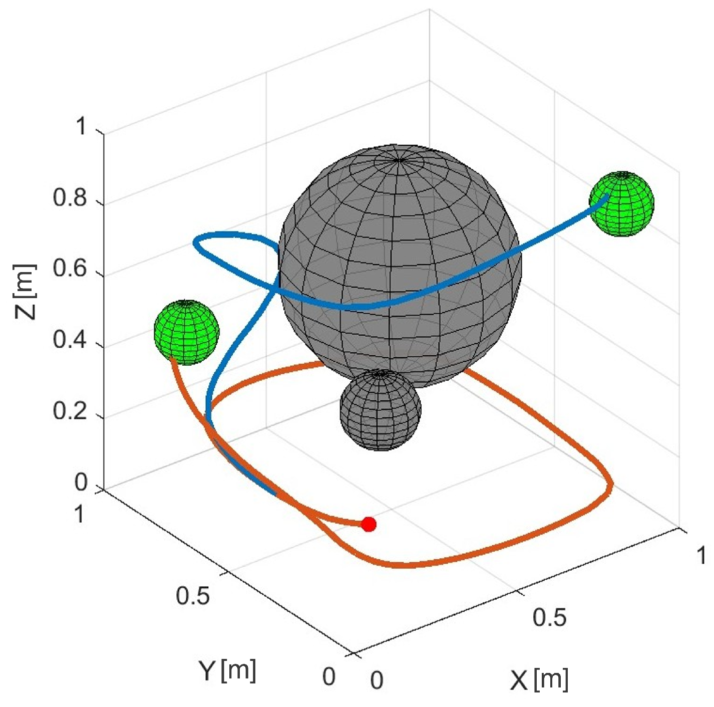
Figure 8 presents two trajectories in the 3D gyre flow environment for a starting configuration of $(x_0,y_0,z_0)=(0.2,0.2,0.2)$ m and goal regions centered at $(x_g,y_g,z_g)=(0.6,0.6,0.6)$ m and $(x_g,y_g,z_g)=(0.35,0.35,0.4)$ m. The tree construction terminated early after reaching both goals at iterations 450 and 674, with a total runtime of only $0.72$ s. In this simulation, the integration step and the maximum integration time were set respectively to $dt=10$ms and $t_{\max }=0.2$s. Though the vehicle is unactuated in lateral directions, it successfully leverages vertical motion to shift between flow layers, enabling lateral repositioning. The curvature of the resulting trajectories illustrates this mechanism, demonstrating how altitude control alone allows access to dynamically favorable flow corridors. This behavior sets the foundation for planning strategies in more realistic planetary environments, such as the atmosphere of Venus.

4.3. Venusian Flow Environment

The Venusian atmosphere presents a compelling testbed for trajectory planning. High-altitude winds on Venus are among the fastest sustained atmospheric flows in the solar system, with zonal (west-to-east) velocities reaching over 300 km/h. In contrast, south-to-north (meridional) winds are comparatively weak and exhibit significant variation with altitude. This directional asymmetry makes Venus an ideal candidate for altitude-controlled drifters, which can exploit vertical wind gradients to steer laterally without requiring direct actuation in all directions.

Motivated by real-world exploration goals such as mapping volcanic activity, studying cloud chemistry, and monitoring climatic evolution, recent research has proposed using underactuated balloon vehicles that ascend or descend to target wind layers for lateral repositioning [22]. To model this scenario, environmental data were extracted from a publicly available climate database [28], which provides wind velocities across all latitudes and longitudes at various altitudes. For this study, the region of interest was bounded between 52 km and 60 km above the Venusian surface, representing the operational band of a typical high-altitude pumped-helium balloon [6].

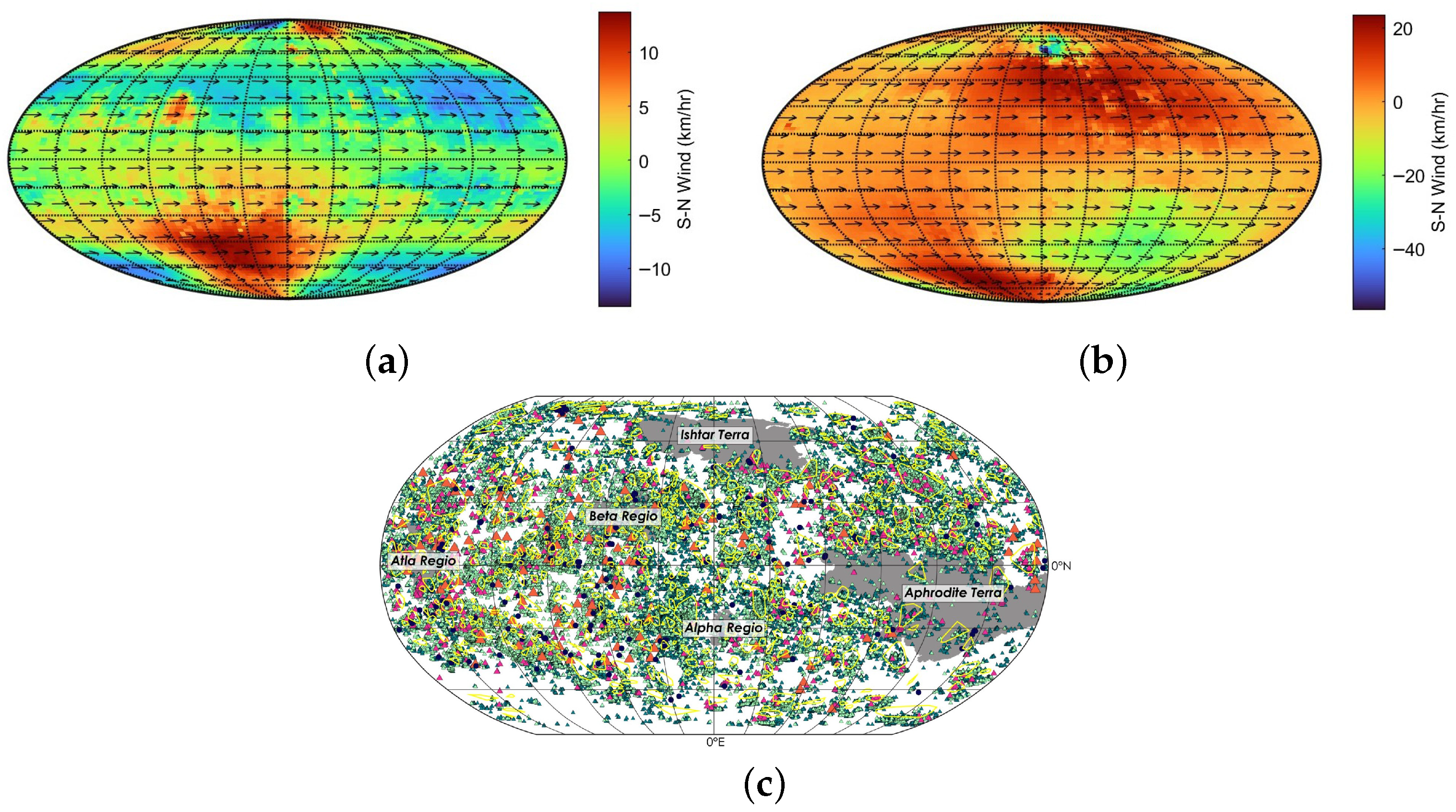
Figure 9 illustrates meridional wind magnitudes at both the lower and upper extremes of this band. Figure 9a,b show that the structure and intensity of south-to-north flow vary significantly with altitude, providing a navigable control channel for underactuated vehicles that can control altitude to passively drift through wind corridors. Figure 9c provides a broader context by displaying over 85,000 volcanic features distributed across the surface, underscoring the scientific value of atmospheric planning capabilities.

The wind field used in our simulations consists of discretized west-to-east, south-to-north, and vertical velocity components at 1 km altitude increments. Vertical motion is governed by both the vehicle’s control inputs and the contribution from the flow field. The vehicle’s vertical acceleration is bounded to reflect its limited actuation capabilities.

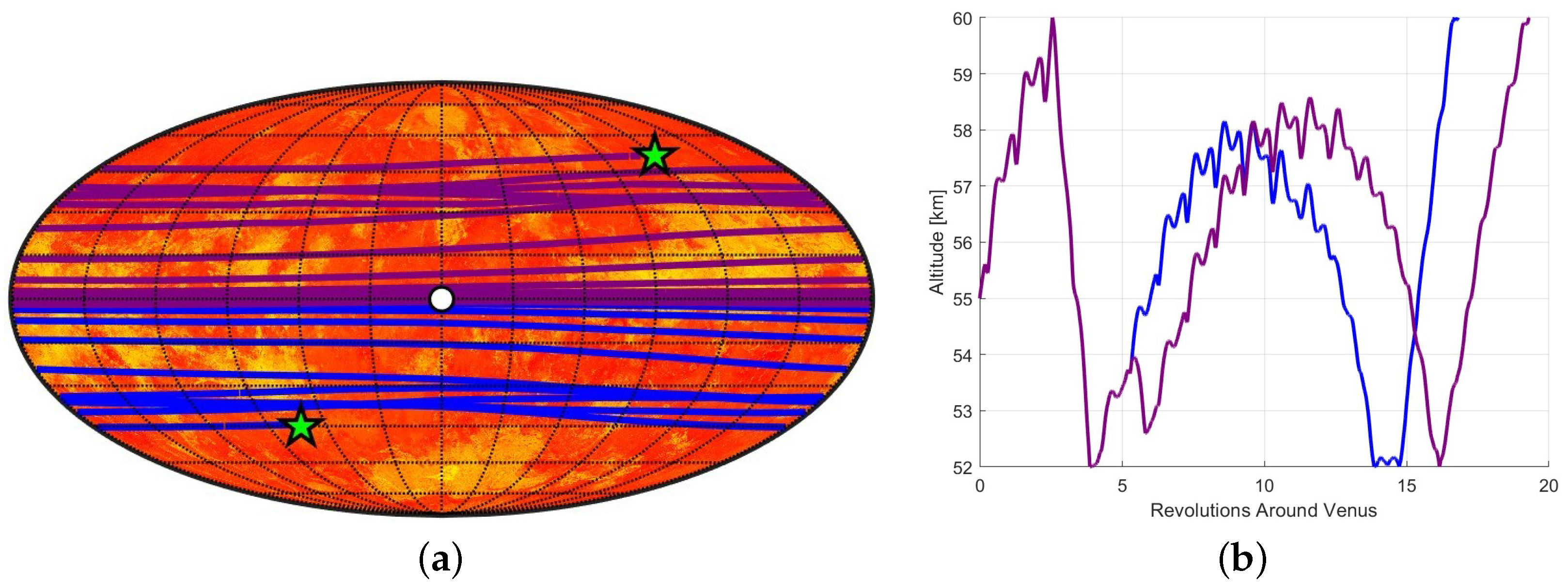
To evaluate planning performance in the Venusian wind environment, a single start point was defined at the planetary equator: $0^{\circ }$ latitude, $0^{\circ }$ longitude, and 55 km altitude. Two goal regions were selected at significantly different latitudes to test the planner’s ability to traverse long distances through the atmospheric flow. The first goal was placed in the southern hemisphere at approximately $-{45}^{\circ }$ latitude and ${285}^{\circ }$ longitude, while the second was in the northern hemisphere at ${51}^{\circ }$ latitude and ${120}^{\circ }$ longitude, both at 55 km altitude. Because the Venus flow field contains strong zonal (east–west) currents, reaching these goals often requires trajectories that circumnavigate the planet while gradually adjusting altitude to align with favorable flow layers.

The algorithm achieves this behavior through discrete vertical actuation, selecting among a set of control inputs to modify altitude. Once a suitable altitude is reached, it relies on minimal actuation and passive drifting to exploit the prevailing wind. This is evident in the sparse, smooth trajectories seen in the resulting plots (Figure 10). The integration time step was set to $dt=10$min, ensuring the flow velocity is queried at regular intervals while allowing consistent forward propagation. For this simulation, the maximum vertical speed of the balloon was set to $v_{r_z}=0.4$ km/h and the maximum vertical acceleration to $a_{r_z}=0.2$ ${\mathrm{km}/\mathrm{h}}^2$, values that are consistent with those for exploratory balloons [25].

Figure 10 presents the resulting trajectories. Remarkably, viable trajectories to both goal regions are discovered within the first 100 samples. Despite the low node count, the trajectories span vast portions of the planetary surface and complete multiple revolutions around Venus. This long-range behavior is enabled by extending the maximum integration time $t_{\max }$ to 2000 h (≈83 days), which naturally increases computational time ($168$s) but proves essential for capturing global-scale transport. It is important to mention that a higher number of samples would not improve the trajectory, which is a common characteristic of RRT-based planning algorithms [26]. Also, a completely different trajectory could be found with a different random seed. Figure 10b shows the altitudinal trajectory of the vehicle for the paths in Figure 10a, which highlights how the proposed algorithm successfully and probabilistically adjusts control commands to traverse both lower and upper atmospheric bands by leveraging the structure of Venusian wind fields to access different latitudinal layers.

5. Conclusions and Future Work

This paper presented a motion planning algorithm for underactuated vehicles operating in environments dominated by strong flow fields. The proposed approach is inspired by RRT, but with sampling directly in the control space, rather than configuration or velocity space. At each iteration, a random node is selected from the tree, and a control input, producing a discrete vertical acceleration, is sampled from a bounded set. This control input is then integrated over time to create a new trajectory segment, ensuring that all sampled trajectories are dynamically feasible and respect both physical actuation limits and the structure of the surrounding flow.

The key contribution of this work lies in embedding feasibility directly into the sampling phase via control-space exploration. This eliminates the need for pruning or post-processing and ensures that each edge in the tree represents a realizable trajectory under the system’s dynamics. Such an approach is particularly effective for underactuated vehicles, where passive directions are governed by environmental forces, and maneuverability is limited to a single actuation axis. By mapping control inputs to trajectory segments through integration, the planner naturally adapts to local flow conditions and maintains compliance with system constraints.

While our current implementation assumes a simplified control model, it already integrates vehicle motion under sampled control inputs, which eliminates the need for straight-line edge assumptions, allowing the planner to produce physically realizable trajectories through forward integration. Without changing the proposed algorithm, the current vehicle’s model used in our experiments can be easily updated to incorporate more realistic system dynamics. This dynamic model can include actuation delays, drag, and acceleration profiles governed by mass and buoyancy, as captured in the detailed models developed by [25], which account for real-world factors such as variable atmospheric density and pressure. These enhancements would allow the planner to more closely reflect the true behavior of the underactuated vehicle and open the door to integrating low-level control models into the planning phase itself.

Although the planner was tested using static wind fields, the underlying framework is well-suited to accommodate temporally evolving flow data. By integrating control inputs over time while querying dynamic flow conditions, the planner could be adapted to forecast trajectories based on future flow predictions. This capability would be particularly valuable for planetary balloons and ocean drifters, where leveraging forecasted environmental changes can improve long-range navigation and energy efficiency. Incorporating time-varying wind or current fields represents a natural and impactful extension of this work.