Article

Physics-Informed Weighting Multi-Scale Deep Learning Inversion for Deep-Seated Fault Feature Identification: A Case Study of Aeromagnetic Data in the Dandong Region

1
Jiangsu Earthquake Agency, Nanjing 210014, China
2
College of Geo-Exploration Science and Technology, Jilin University, Changchun 130012, China
*
Author to whom correspondence should be addressed.
Appl. Sci. 2025, 15(22), 12323; https://doi.org/10.3390/app152212323
Submission received: 15 September 2025 / Revised: 6 November 2025 / Accepted: 17 November 2025 / Published: 20 November 2025
(This article belongs to the Section Earth Sciences)

Abstract

Magnetic inversion through three-dimensional (3D) susceptibility reconstruction can effectively identify the deep extension characteristics and structural variations in faults. Therefore, the reliability of inversion results from magnetic anomaly data is a key issue that must be addressed in fault detection and quantitative evaluation of fault activity. In recent years, deep neural network-driven magnetic data inversion methods have rapidly become a research focus in the field of geophysical magnetic data inversion. However, existing methods primarily rely on convolutional neural networks (CNNs), whose inherent local feature extraction capabilities limit their ability to model the spatial continuity of large-scale subsurface magnetic structures. Moreover, the general lack of prior physical constraints in these network models often leads to unreliable inversion results. To address these limitations, this paper proposes a physics-informed multi-scale deep learning inversion method for magnetic anomaly data. The method designs a dual-stream Transformer-CNN fusion module (TCFM). It leverages the self-attention mechanism in Transformers to model global susceptibility correlations while efficiently capturing local geological features through CNN convolutional operations. This enables collaborative modeling of multi-scale subsurface magnetic structures, significantly enhancing inversion accuracy. Furthermore, by incorporating deep physical priors, we design a depth-aware weighted loss function. By strengthening optimization constraints in deep regions, it effectively improves the vertical resolution of inversion models for deep magnetic structures. Comparative experiments with U-Net++ and Transformer demonstrate that the proposed method achieves smaller errors and higher inversion accuracy. Applied to measured aeromagnetic data from the Dandong region of China, the method yields reliable inversion results. Variations in magnetic susceptibility within these results successfully delineate the spatial distribution of fault zones, providing a geophysical basis for regional seismic hazard monitoring and assessment.

1. Introduction

Magnetic anomaly inversion is a key technique in geophysical exploration, widely used in underground resource exploration, seismic monitoring, structural analysis, and fault identification. By inverting surface magnetic anomaly data, it is possible to reveal the distribution of underground magnetic susceptibility, which helps in understanding the structural characteristics of underground rocks [1,2,3,4,5,6]. Magnetic anomaly inversion is particularly important in the study of fault systems, as abrupt variations in magnetic susceptibility can effectively indicate fault depth, structural properties, and stress accumulation, providing crucial technical support for the study of earthquake generation mechanisms [7,8,9].
In recent years, with the rapid advancement in computational capabilities and data processing technologies, magnetic anomaly inversion methods have rapidly developed. Traditional inversion methods typically rely on physical models to solve magnetic field inversion problems to infer the distribution of underground magnetic sources. While these methods provide theoretical foundations, they often face challenges related to the high dimensionality of parameters and inversion instability, especially when dealing with complex geological structures [10]. With the rise in deep learning (DL) technologies, data-driven methods have emerged as a new solution. Deep learning methods can reconstruct subsurface structures directly from data without relying on initial models, thus overcoming the limitations of traditional methods [11,12,13].
In particular, Convolutional Neural Networks (CNNs) and Transformer models, due to their powerful nonlinear modeling capabilities and global optimization abilities, have achieved significant success in magnetic anomaly inversion [14,15,16,17,18]. However, these methods typically focus on global features and may have limitations in capturing fine local geological structures. Thus, how to combine both global and local information to improve inversion accuracy has become a key challenge in the field of magnetic anomaly inversion.
To address these challenges, this paper proposes a physics-informed multi-scale deep learning inversion method, combining the advantages of Transformer and CNN models, and designing an innovative dual-stream fusion module (TCFM). This method can simultaneously model global dependencies of magnetic susceptibility and local geological structural features, thereby improving inversion accuracy and depth resolution. By comparing this method with existing deep learning-based approaches, the results demonstrate significant advantages in reducing inversion errors and improving the resolution of deep structures.

2. Literature Review

Magnetic anomaly inversion methods have developed in two main directions: physics-driven methods and data-driven methods. Physics-driven methods rely on magnetic field laws and regularization techniques to discretize the subsurface into magnetic units and match the observed data with theoretical magnetic field values through optimization, thus inferring the distribution of underground sources. These methods have been dominant in magnetic anomaly inversion in the early stages, particularly the Tikhonov regularization method [19,20] and depth-weighted constraint methods [21,22]. These methods improve inversion accuracy and stability by introducing additional geological or spatial gradient constraints. However, despite their progress, traditional physics-driven methods still have limitations, especially when dealing with complex geological environments, as they often heavily depend on the quality of the initial model and may suffer from local minima during optimization, affecting solution reliability.
With the rapid development of deep learning technologies, data-driven methods have gradually become a promising alternative for magnetic anomaly inversion. Deep learning methods, particularly CNNs and Transformer models, are highly effective in learning from large datasets and can model complex nonlinear relationships without the need for initial models. For instance, Deng et al. [17] proposed a CNN-based method for inverting 3D magnetic gradient tensors, significantly improving inversion accuracy. Shi et al. [23] introduced deep learning-based 3D inversion approaches using multiple magnetic datasets, improving inversion precision. Despite the success of these CNN-based methods [24,25], they are limited by their finite receptive fields, which restrict their ability to model long-range dependencies and global context, thus neglecting the long-range influences of magnetization at different depths [26]. To overcome these challenges, Transformer models have attracted increasing attention. Transformer models, known for their excellent ability to capture global dependencies, have been successfully applied in various fields, including geophysics. Jiang et al. [27] and Gao et al. [28] applied Transformer models to seismic data and impedance inversion, respectively, demonstrating their advantages in modeling global features. However, Transformer models also have drawbacks in modeling local information, which limits their effectiveness in capturing fine geological structures [29].
Therefore, combining the strengths of CNNs and Transformer models to simultaneously model both global and local features has become an important direction in the research of magnetic anomaly inversion. The dual-stream fusion module (TCFM) proposed in this paper aims to address this issue. By integrating the global modeling capability of Transformers and the local feature extraction capability of CNNs, TCFM can more accurately invert complex subsurface magnetic structures.
Despite the significant progress made by deep learning methods in inversion accuracy, most existing methods still lack physical constraints, which can make them unreliable in accurately revealing deep magnetization structures under complex geological conditions. Recently, more and more studies have explored combining physical priors with deep learning models, using physical constraints to optimize the inversion results. This combined approach not only helps improve the resolution of deep features but also enhances the reliability of the inversion results.

3. Methods

3.1. Inverse Problem

Physics-driven methods infer subsurface magnetization models based on a regularization framework combined with optimization algorithms [30,31]. For computational convenience, we assume that the target bodies are vertically magnetized. Under this assumption, the magnetic anomaly generated by an anomalous body can be calculated using the following formula [6]:
T = μ 0 M 4 π ( ζ z ) a r c t a n ( x ξ ) ( y η ) r ( z ζ ) | ξ 1 ξ 2 | η 1 η 2 | ζ 1 ζ 2 ,
Here, μ 0 is the magnetic permeability, M is the magnetization intensity, ξ, η, ζ represent the coordinates in the x, y, and z directions, respectively, and r is the distance from the volume element to the observation point. If the subsurface space is discretized into regular cubic cells, the problem can be simplified as:
d = A m ,
where d represents the magnetic anomaly, m denotes the physical property parameters (magnetic susceptibility), and A is the sensitivity matrix [5,6].
DL requires a large amount of m and d data to train the neural network and establish a complex mapping relationship between them [32,33,34], allowing the direct estimation of m . This mapping can be expressed as:
m ~ = N e t s ( d , θ ) ,
where m ~ is the predicted magnetic susceptibility model, N e t s represents the neural network, and θ denotes the network parameters. During network training, the parameters θ are optimized using the backpropagation algorithm [35] to minimize the output error, following the principle:
θ ^ = arg m i n θ 1 N i = 1 N L ( m i , N e t s ( d i , θ ) ) .
where L denotes the loss function, N is the size of the training dataset, and ( m i , d i ) represents the i-th sample pair in the dataset.

3.2. Network

CNN-based network models are constrained by their limited local receptive fields, making it difficult to effectively capture the global spatial relationships of subsurface magnetic susceptibility distributions. On the other hand, Transformer-based (TF-based) models, while capable of establishing global dependencies through self-attention mechanisms, tend to overlook the fine-grained representation of local details. The limitations of both approaches can result in reduced inversion accuracy. To address these issues, this paper proposes a deep learning framework based on a global-local collaborative mechanism. The overall architecture is illustrated in Figure 1.
The input magnetic anomaly observation data d is first processed by a 1 × 1 convolutional layer to extract low-level features related to magnetization variations, generating the initial feature map F . Next, F is downsampled using a max-pooling operation, producing a feature map F 1 with half the original size. F 1 is then fed into the TCFM, the structure of which is shown in Figure 1.
In the TCFM, F 1 is simultaneously passed through two branches: a local feature extraction branch and a global feature extraction branch. These are used to capture the detailed variations in geological structures and the global dependencies of magnetization, respectively, producing a local feature map F l and a global feature map F g .
F l = B N L R ( F 1 + ( C o n v ( B N L R ( C o n v ( F 1 ) ) ) ) ) ,
Among them, BNLR refers to BatchNorm and Leaky ReLU, and Conv denotes a convolutional layer with a 3 × 3 kernel size.
The global feature extraction branch first applies a Patch Partition operation to divide F1 into non-overlapping patches of size p × p × p (with p = 4 in this study), followed by serialization and tokenization (feature vector mapping), laying the foundation for capturing spatial correlations in the magnetic anomalies. Each token is multiplied by corresponding matrices to obtain a query q i , key k i , and value v i . Then, Layer Normalization (LN) and Multi-Head Self-Attention (MSA) are applied to model the long-range spatial dependencies among magnetization values, enhancing the representation of continuity in complex geological structures. The self-attention mechanism is processed as follows [36]:
A t t e n t i o n Q , K , V = s o f t m a x Q K T d V ,
All q i , k i and v i are assembled into matrices Q , K , and V , respectively. The output of the self-attention mechanism is obtained by a weighted summation of Q , K , and V , enabling the network to dynamically attend to features across all positions in the sequence when processing magnetic anomaly data. This allows for effective modeling and extraction of global dependencies in magnetic anomalies. Finally, the global features are passed through a linear projection layer within an MLP to restore the spatial dimensions to match the input, producing the global feature map F g . As shown in the following formula,
F g = A t t e n t i o n ( F 1 )
The overall process of global modeling can be described as follows:
F g = M S A L N F g 1 + F g 1 F g 1 = M L P L N F g + F g
To enhance the model’s ability to interpret complex magnetic anomaly sources, this global modeling process is stacked multiple times within the network, enabling more effective fusion of global magnetization features.
Subsequently, the local feature map F l and the global feature map F g are fused through a convolutional layer, effectively integrating local spatial characteristics of the source with global magnetization dependencies. This enhances the model’s ability to perceive magnetic anomaly features at multiple scales and improves the accuracy of the inversion results. Finally, a 1 × 1 convolutional layer is used to output the 3D magnetization model, achieving an effective inversion from magnetic anomaly observation data to the subsurface magnetization distribution.

3.3. Physical Constraint Loss Function

In deep learning-based magnetic inversion, the loss function is used to evaluate the error between the reconstructed subsurface magnetic susceptibility distribution and the true susceptibility distribution. In this study, a novel depth-aware weighted loss function is introduced, which dynamically adjusts the weighting coefficients of the loss, guiding the model to focus on learning the features of deep magnetic bodies. By deeply integrating physical constraints with data-driven learning, this approach enhances the vertical spatial resolution and reliability of the inversion results.
In conventional deep learning-based magnetic inversion methods, the Mean Squared Error (MSE) loss function is commonly employed [18,19,20], as defined by the following equation:
L M S E = 1 N i = 1 N | | m i m i ~ | | 2 ,
Due to the physical characteristic of rapid signal attenuation with depth in magnetic anomalies, the MSE loss function exhibits significant limitations when applied to the in- version of deep magnetic susceptibility distributions. As shown in Equation (8), the MSE loss assigns equal weight to all subsurface grid cells. As a result, shallow magnetic bodies, which produce strong anomaly signals, dominate the gradient updates during training. This leads the network to prioritize minimizing errors in shallow regions, while the weak signals from deeper areas provide insufficient gradient information to effectively guide the network in learning deep features. Consequently, the inversion results lack adequate vertical resolution.
To address this issue, this study introduces a depth-aware weighted loss function, which assigns higher weights to deeper subsurface grid cells. This encourages the network to be more sensitive to errors in deeper regions during training, thereby directly compensating for the attenuation of deep signals caused by the physical decay of the field. As a result, the network’s ability to perceive and reconstruct deep magnetic structural features is significantly enhanced, improving the vertical resolution of the inversion results. The loss function is defined as follows:
L D e p t h = 1 1 + e 1 z | m i m i ~ |                       z =   1 16 ,
The final composite loss function is expressed as:
L = L M S E + α L D e p t h .
where     α is weighting coefficients, which must be empirically determined through multiple experiments [37,38,39,40]. In this study, we set   α = 0.01.

3.4. Dataset Construction and Network Training

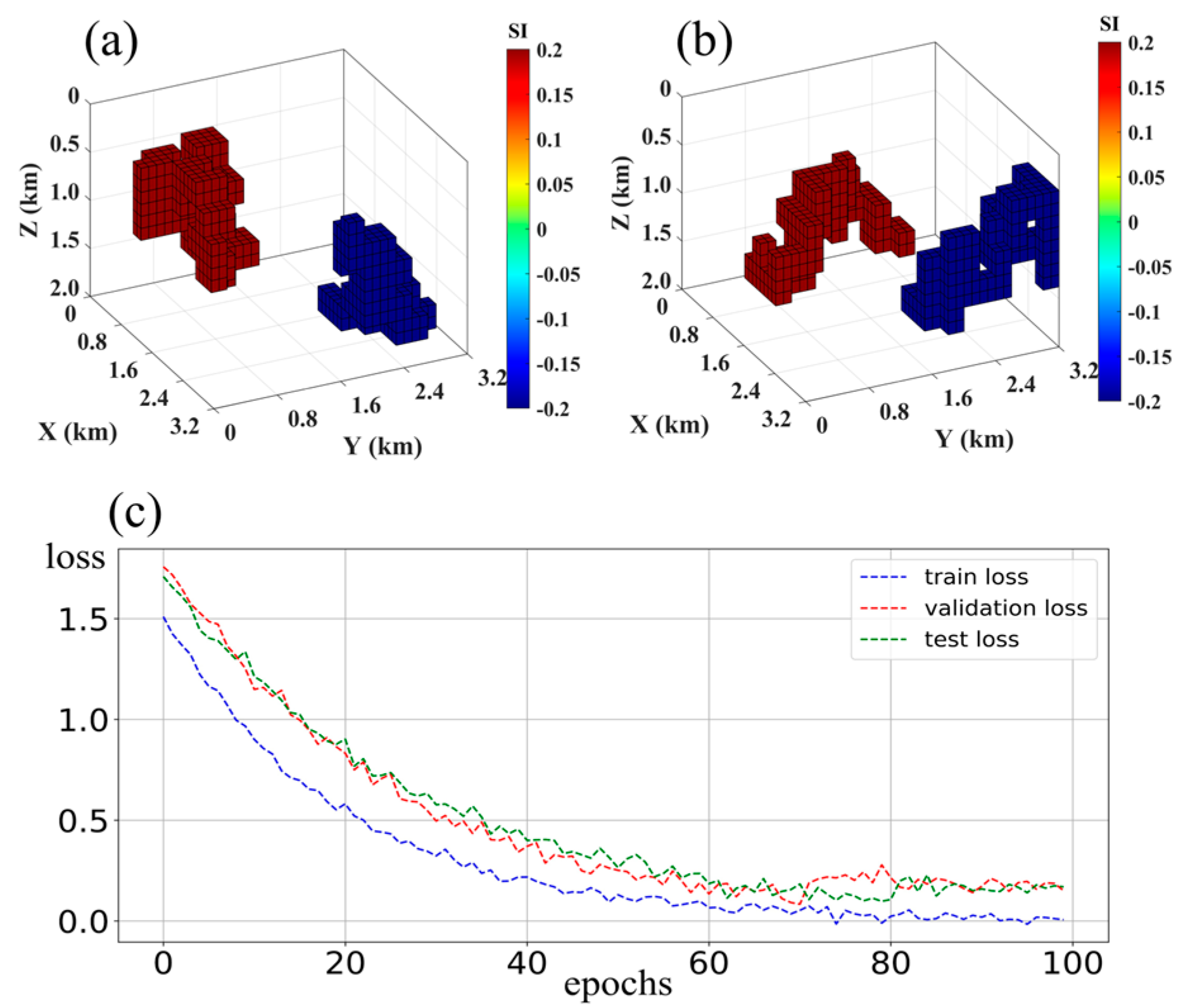
In this study, the subsurface space was divided into 32 × 32 × 16 cubes. To match the size of the survey area, each cube was set to a size of 1.00 × 1.00 × 0.7 km. A total of 30,000 random models were generated using a combination of the random walk method and forward modeling algorithms (Equation (1)), and their corresponding magnetic anomaly data were calculated (see Figure 2). These data were used as the basis for the training and validation sets. The magnetization of the models was set to ±0.2 SI with the background field fixed at zero. The subsurface space was symmetrically divided into four regions (top, bottom, left, right). For each model, a random starting point was selected from at least one of the regions, and then moved one step in a randomly chosen direction for a total of s steps (s ranging from 40 to 80). This process generated a 3D model. The randomness of this method enables the simulation of various complex magnetic sources, providing reliable data support for subsequent network training.
Additionally, 2000 irregular models that do not overlap with the training set were generated as the test set. All data were fed into the network in a 14:1:1 ratio. The network loss curve is shown in Figure 2c.
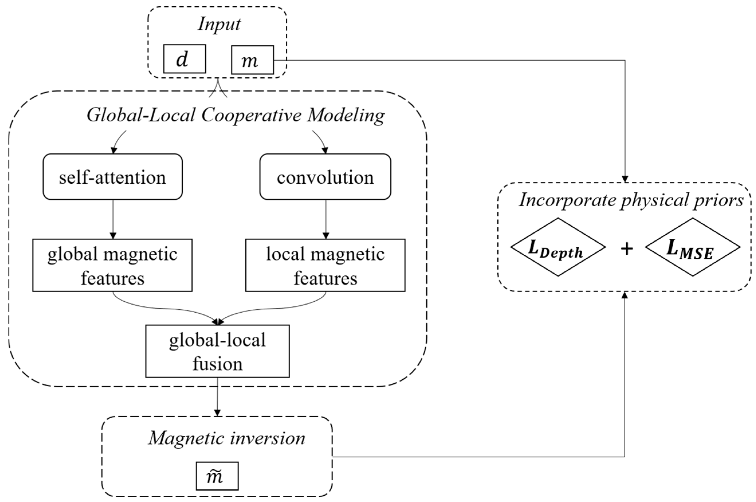
During the training phase, a batch size of 32 was used, the learning rate was set to 3 × 10⁻³, and a dropout rate of 0.1 was applied. The Adam optimizer was employed to adjust the network parameters, and the model was trained for a total of 100 epochs. Table 1 summarizes the computational efficiency comparison between the Transformer-CNN model, U-Net++, and traditional Tikhonov inversion. The GPUs used were NVIDIA A100. The workflow of the proposed inversion method is illustrated in Figure 3. Magnetic anomaly data are processed through collaborative modeling of global-local magnetic features using self-attention and convolution mechanisms. Combined with the integration of physical priors via the depth-aware weighted loss function, this approach ultimately enables high-precision three-dimensional inversion of complex subsurface magnetic structures.

4. Model Testing

4.1. Evaluation Metrics

This study uses two metrics—model fit and data fit—to evaluate the performance of different inversion methods. The model fit is used to measure the difference between the inverted model m ~ and the actual geological model   m , expressed as follows:
E m = | | m ~ m | | 2 2 | | m | | 2 2
Data fitting degree is used to measure the error between the forward anomalous data d ~ corresponding to the inversion model mm and the true anomaly d , as shown below:
E d = | | d ~ d | | 2 2 | | d | | 2 2
The false anomaly rate can intuitively measure the proportion of false anomalies in the predictive model. The formula is as follows:
F P R = F P V T V M × 100 %
where FPV is the absolute difference in magnetic susceptibility between the predicted and true model exceeds 0.05 SI and lies outside the true anomaly regions. TVM is all voxels in the true anomaly region of the model.
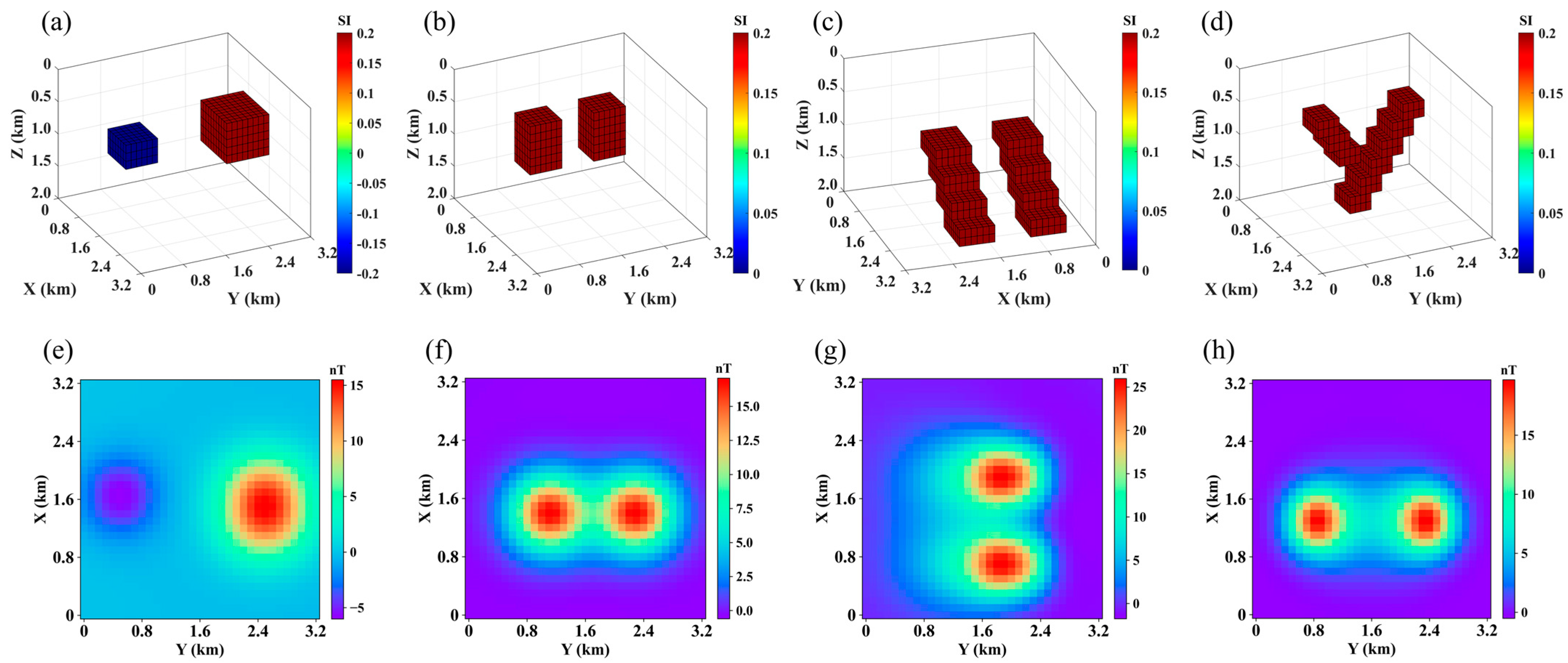
Four synthetic models were established in this study to validate the proposed method, as shown in Figure 4. Furthermore, comparative experiments were conducted with the CNN-based U-Net++ and the Transformer-based Vision Transformer (ViT) to better demonstrate the advantages of our approach.

4.2. Test Model Analysis

4.2.1. Test Model One

Model One consists of two horizontal prisms with magnetic susceptibilities of 0.2 SI and −0.2 SI, respectively, both centered at a depth of 0.32 km. Figure 5a–c show the inversion results obtained using the proposed method, U-Net++, and ViT, respectively. It can be observed that all three inversion methods produce low-amplitude spurious anomalies for models with different magnetic susceptibilities. However, the proposed method significantly reduces the number of such artifacts and yields more concentrated physical property distributions, demonstrating superior capability in property recovery. In contrast, the results from U-Net++ and ViT exhibit more spurious anomalies and relatively scattered property distributions. The FPR was found to be 3.2% for the proposed method, 8.5% for U-Net++, and 6.9% for ViT. The model fitting errors for the proposed method, U-Net++, and ViT are 0.064, 0.126, and 0.112, respectively, indicating a clear advantage in model fitting accuracy for the proposed approach. Figure 5d–e display the forward-modeled magnetic anomalies derived from the inverted models of the proposed method, U-Net++, and ViT. The morphology and amplitude of the forward responses from all three methods are generally consistent with the true anomaly. However, the proposed method produces a forward response that aligns more closely with the true data in detail. The corresponding data misfit errors are 0.213, 0.541, and 0.387, respectively, confirming that the proposed method achieves higher data fitting accuracy.

4.2.2. Test Model Two

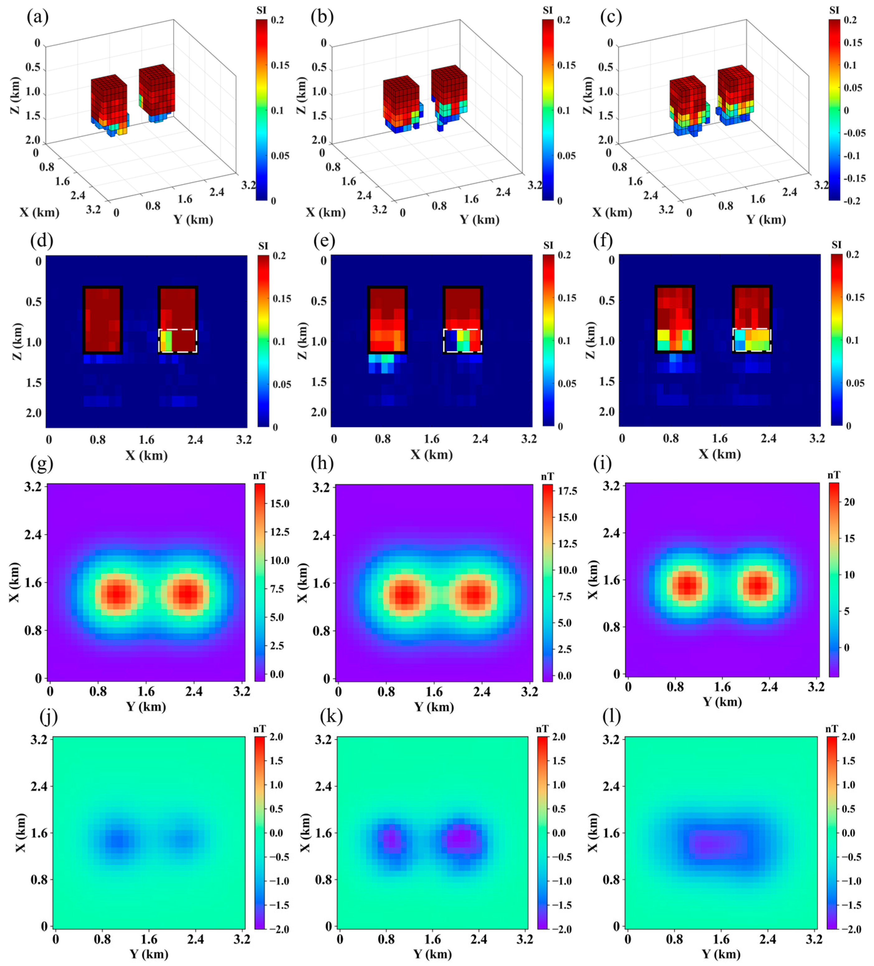
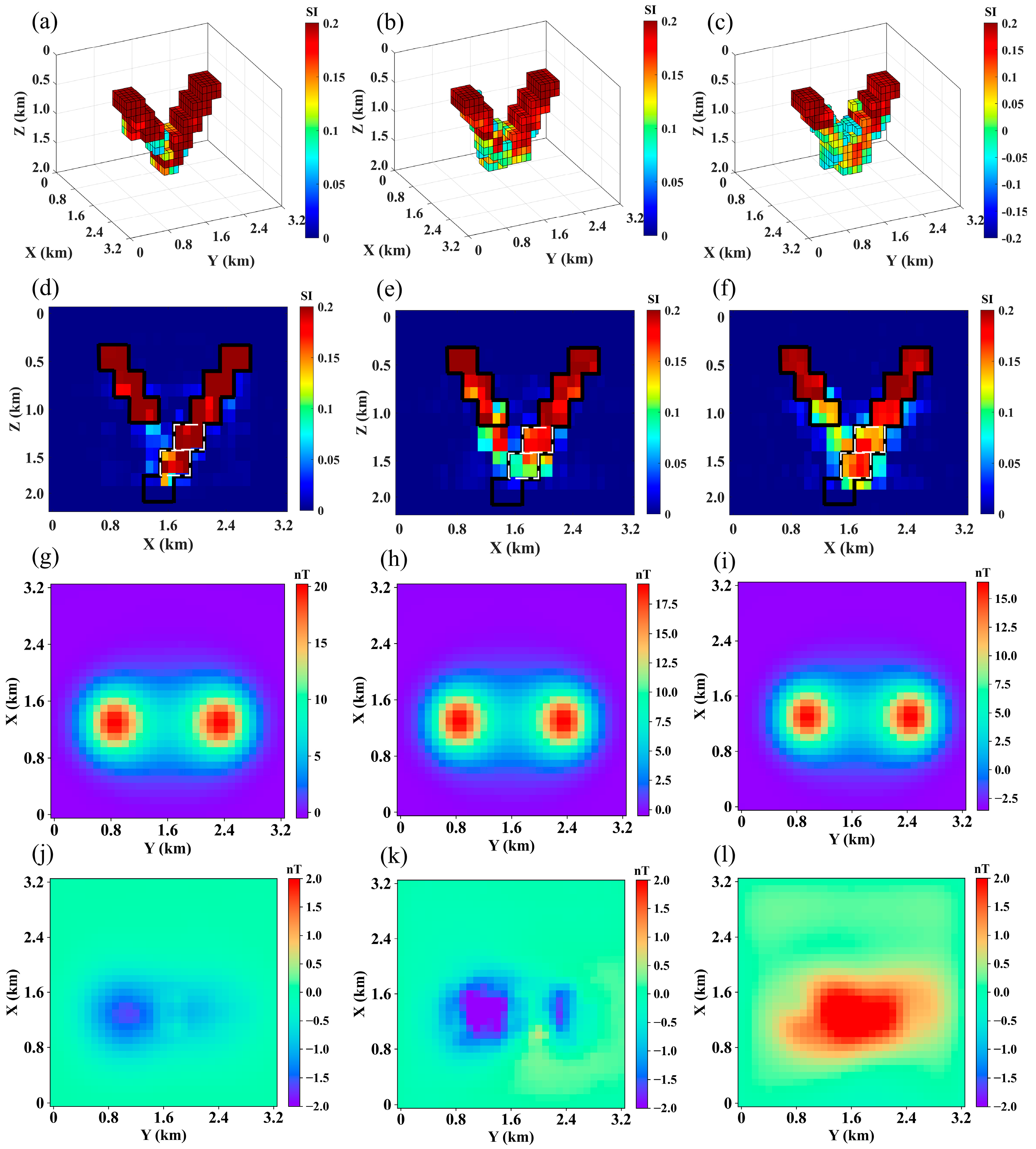
Model Two consists of two cubes of identical dimensions and burial depths, both with a magnetic susceptibility of 0.2 SI and centered at a depth of 0.45 km. The inversion results and cross-sectional views are shown in Figure 6, with the profile taken at X = 1.2 km. Comparative analysis indicates that U-Net++ performs relatively well in shallow regions, but exhibits noticeable magnetic discontinuities and localized susceptibility loss in deeper zones, as highlighted by the white dashed boxes, which limits the completeness and accuracy of the model reconstruction. Although ViT demonstrates better global recovery capability than U-Net++, it still shows certain degrees of discontinuous susceptibility distribution. In contrast, the proposed method yields superior performance in recovering deep structures. The inversion result shows more continuous susceptibility distribution, higher resolution of deep features, and no missing susceptibility values, enabling accurate reconstruction of the entire model’s structural characteristics. The FPR was 4.5% for the proposed method, 9.0% for U-Net++, and 7.8% for ViT. The model fitting errors for the proposed method, U-Net++, and ViT are 0.098, 0.250, and 0.175, respectively. Furthermore, Figure 6g–i present the magnetic anomalies of the true model, the proposed method’s inverted model, and the U-Net++ inverted model, respectively. Comparison reveals that the forward responses of both U-Net++ and ViT exhibit significant deviations from the true anomaly, whereas the proposed method produces a forward response that aligns more closely with the true data in both magnitude and morphology. The corresponding data misfit errors are 0.359, 0.816, and 0.562, respectively.

4.2.3. Test Model Three

Model Three is a complex model composed of two synclinal prisms, each with a magnetic susceptibility of 0.2 SI and a top burial depth of 0.56 km. As can be observed from the inversion results (Figure 7), the proposed method outperforms both conventional U-Net++ and ViT in terms of resolution, particularly in deeper regions, where the number of low-amplitude spurious anomalies is significantly reduced. To further evaluate the accuracy of the inversion results, a cross-section was taken at X = 2.3 km and the inversion outcomes along this profile were compared. Compared with other models, our method exhibits more consistent susceptibility distributions. In contrast, the inversion result from the proposed method shows more concentrated susceptibility distribution with values closer to the ground truth, demonstrating higher stability and reliability. The FPR was 3.8% for the proposed method, 8.3% for U-Net++, and 7.2% for ViT. In terms of model fitting error, the proposed method, U-Net++, and ViT achieved errors of 0.383, 0.694, and 0.512, respectively, further validating the superior inversion capability of our approach. Additionally, Figure 7g–i display the magnetic anomalies of the true model and the forward responses of the three inverted models, with corresponding data misfit errors of 0.799, 1.186, and 0.973. The proposed method yields a forward response that outperforms both U-Net++ and ViT in terms of fitting accuracy and consistency.

4.2.4. Test Model Four

Model Four consists of two synclinal prisms of different sizes, both with a magnetic susceptibility of 0.2 SI and a top burial depth of 0.11 km. As observed in the inversion results and cross-sectional views (Figure 8), the U-Net++ model exhibits significant limitations under such complex structural conditions. Specifically, it demonstrates low vertical resolution, difficulty in accurately resolving deep structures, and the presence of numerous unrealistic spurious anomalies, which collectively reduce the reliability of the overall model interpretation. ViT outperforms U-Net++ in recovering the global magnetic structure but still suffers from certain false anomalies and discontinuous physical property distributions. The proposed method demonstrates stronger capability in handling this type of complex model. On one hand, it significantly reduces spurious anomalies and achieves better performance in structural preservation; on the other hand, it markedly improves vertical resolution and allows more accurate restoration of deep susceptibility distributions, as highlighted within the white dashed boxes. Furthermore, the inverted model shows higher consistency with the true model in structural boundary recovery, resulting in a more faithful reconstruction. The FPR was 3.5% for the proposed method, 8.2% for U-Net++, and 7.1% for ViT. The model fitting errors for the proposed method, U-Net++, and ViT are 0.523, 0.806, and 0.774, respectively, demonstrating the superiority of our approach. The corresponding data misfit errors are 1.012, 1.684, and 1.326.

4.3. Noise Robustness Test

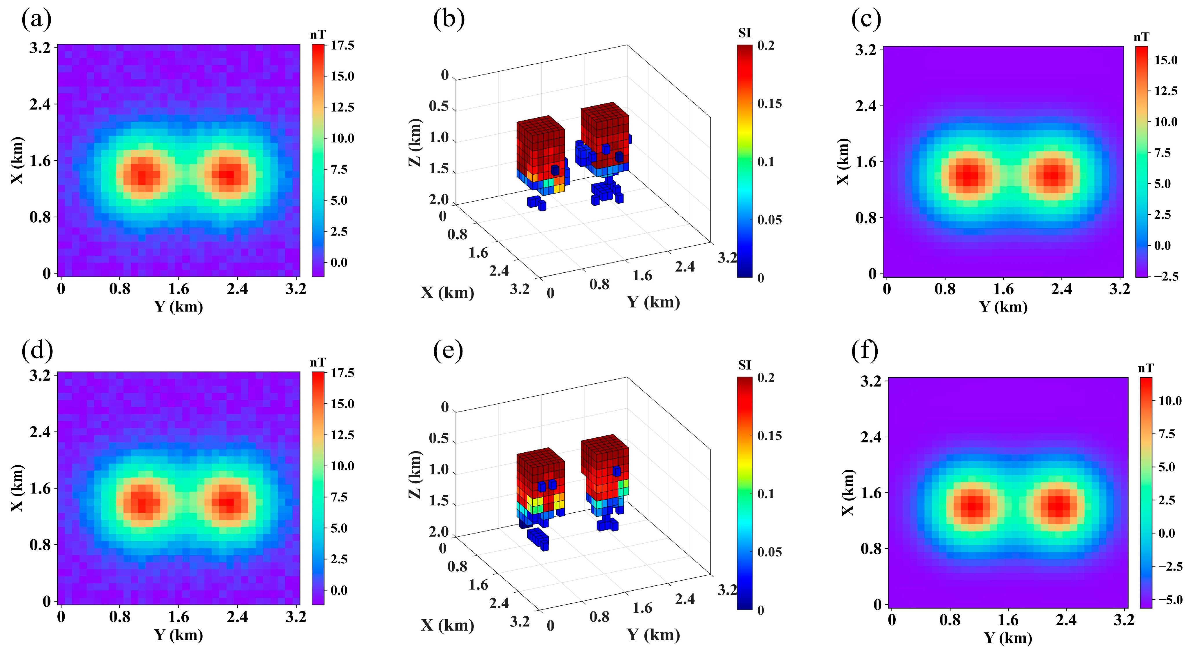
To evaluate the robustness of the proposed method under noise interference, a simulated experiment was designed to approximate real-world observation conditions. During the training phase, 2% and 4% Gaussian noise was added to the training samples, while 6% noise was introduced into the test data. Both the proposed method and the U-Net++ model were trained and validated under these conditions. Figure 9 illustrates the inversion results of each model under this noisy scenario. The experimental results indicate that although the presence of noise slightly affects inversion accuracy, the main geological features—such as magnetization values and spatial locations—can still be reconstructed with reasonable accuracy. This demonstrates that both the proposed method and U-Net++ exhibit good noise resistance. Notably, the proposed method shows higher stability across different noise levels, producing more consistent inversion results and further confirming its robustness advantage.

4.4. Ablation Study

To further demonstrate the advantages of the proposed loss function, the network framework shown in Figure 2 was trained separately using the proposed loss function and the MSE loss function, followed by error analysis. The results are presented in Table 2. As shown, the inversion errors of the method constrained by the proposed loss function are consistently lower than those constrained by the MSE loss function, indicating that the proposed loss function can effectively improve the accuracy of the inversion results.

5. Field Data

The Dandong region is located in the southeastern part of Liaoning Province, China (Figure 10a). It lies on the northeastern margin of the North China Craton, forming the core area of the Jiaoliao Block and representing a key component of the craton. The geological map of the area is shown in Figure 10b. With a geological history spanning more than 3.8 billion years, Dandong serves as a crucial window for studying the tectonic evolution of East Asian continental blocks. As a cratonic margin, Dandong has undergone multiple tectonic events, particularly during the Mesozoic era, when the continuous subduction of the Pacific Plate beneath the Eurasian Plate induced multi-stage deformation and magmatic activity in the region. Structurally, Dandong is situated in the hanging wall of the north-dipping Dabie-Sulu suture zone. This unique location subjected the region to complex deformation and magmatism during the Mesozoic, driven by the subduction of the Paleo-Pacific Plate. Around 195–193 Ma, the region experienced its first major deformation event, followed by partial melting of Paleoproterozoic magmatic rocks around 160 Ma, likely caused by remelting of the lower crust. The multiple deformation phases during the Mesozoic reflect a complex tectonic strain regime, with two significant events occurring at 195–193 Ma and 153–145 Ma. The subduction of the Pacific Plate triggered regional orogeny and the development of fault systems, among which the NE-trending Jixinggou Fault Zone is a major seismogenic structure that has historically produced moderate to strong earthquakes. Between 180 Ma and 145 Ma, the region transitioned from a compressional to an extensional regime, related to changes in subduction direction. From 135 Ma to 95 Ma, frequent activity along NE-trending sinistral faults occurred. These reactivated faults not only served as channels for crustal stress release but also represent preferred orientations for present-day seismic swarms. They controlled the formation of Early Cretaceous extensional basins and facilitated the intrusion of metamorphic core complexes and magmatic rocks, providing a geological basis for mineral resource enrichment [41,42,43,44]. Therefore, research on this region is of significant scientific importance.
In this study, field operations were conducted using a DJI multi-rotor UAV equipped with an aeromagnetic survey system (Figure 11a). The system used in this study was GTK-QTFM-B optical pump magnetometer, sensitivity: 0.02 nT/Hz, resolution: 0.0001 nT and Manufacturer: Shenzhen Jiataike Technology Co., Ltd., China, Shenzhen. The survey area has a relatively regular shape, covering approximately 20 square kilometers. Figure 11b shows the map of the surveyed region. Survey lines were arranged in an east–west direction with a line spacing of 100 m. The UAV maintained a constant flight altitude of approximately 100 m above ground level using terrain-following flight mode, ensuring consistent altitude during the data acquisition process. The flight path is shown in Figure 11c.
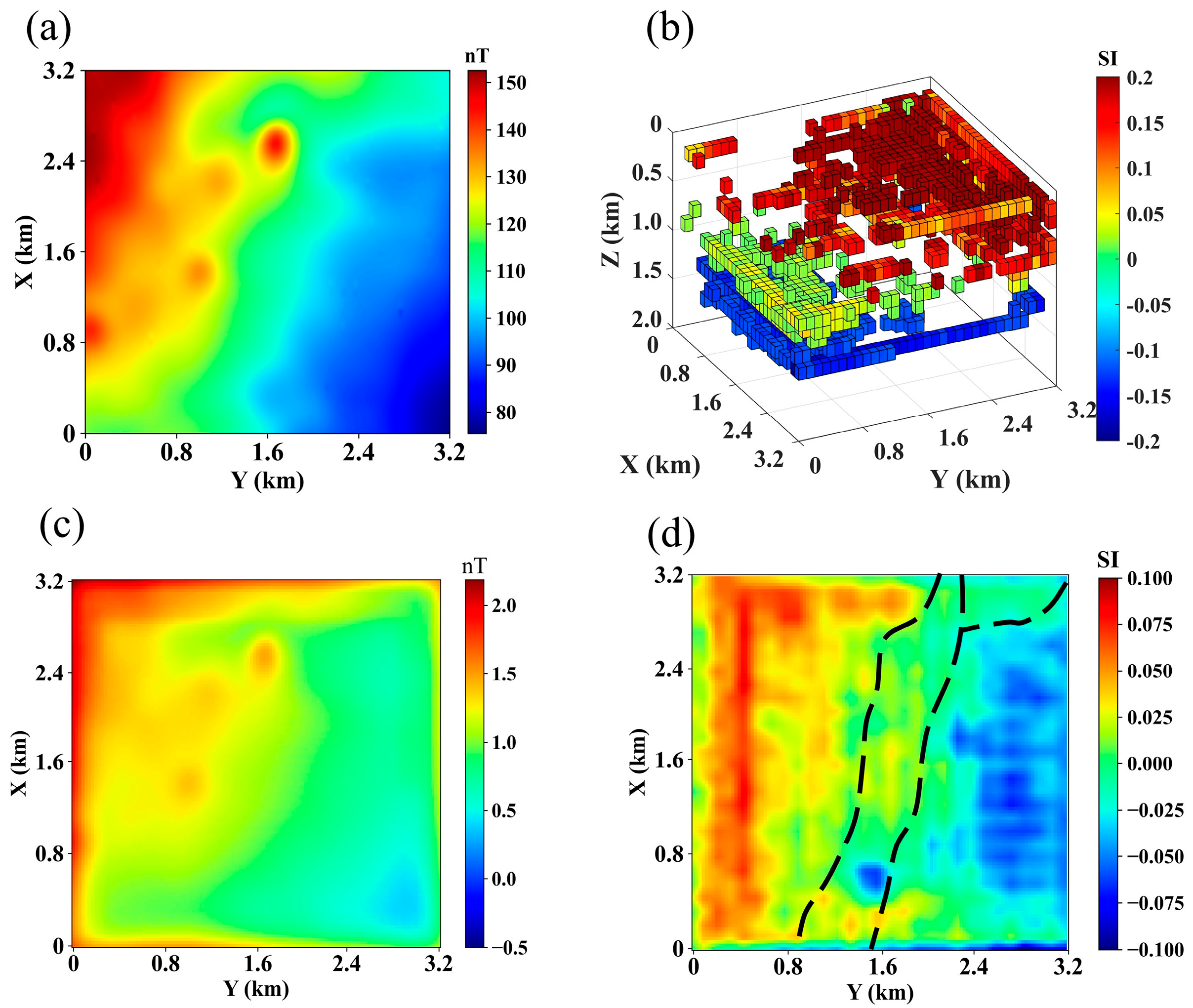
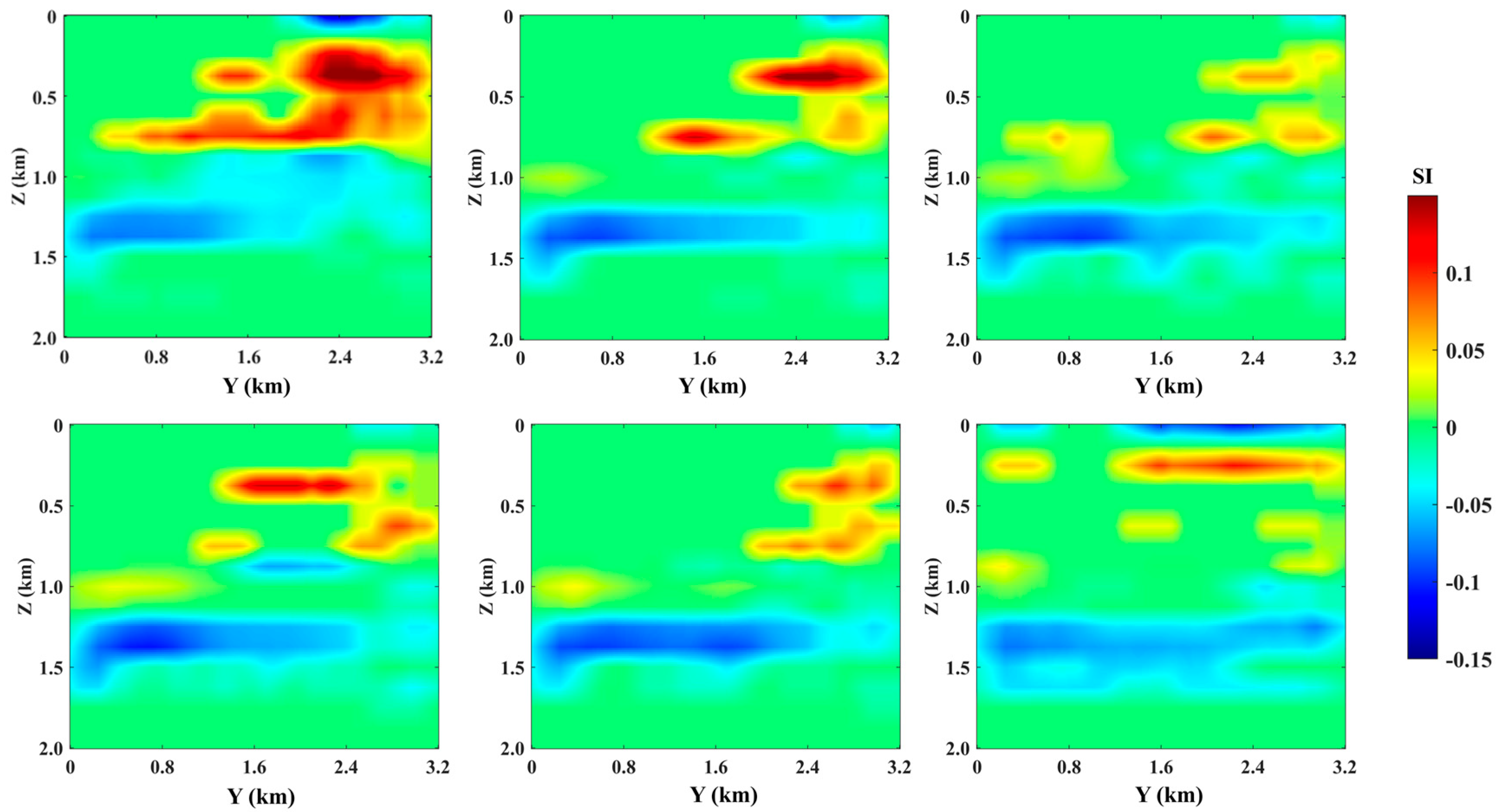
Magnetic anomaly data were obtained from the measured data after a series of processing steps, such as diurnal variation correction, normal field correction, and magnetic pole correction, as shown in Figure 12a. The proposed deep learning-based magnetic inversion method was applied to perform a three-dimensional inversion, yielding spatial distribution information that reflects subsurface structures and lithological variations. The inversion results are presented in Figure 12b, where the magnetic anomalies exhibit distinct vertical layering characteristics: predominantly positive magnetic anomalies in shallow regions and negative anomalies at greater depths, revealing a clear vertical magnetic stratification in the study area. Figure 12c displays the residual map between the forward-modeled magnetic anomalies from the inversion results and the measured magnetic anomalies. The overall small residuals validate the stability and reliability of the inversion model. To more intuitively identify fault features, the 3D susceptibility results were projected onto the XY plane, as shown in Figure 12d, where the black dashed lines indicate the inferred fault locations. The figure reveals significant magnetic contrasts in the east–west direction: the western region is characterized by low magnetic anomalies (susceptibility approximately −0.08), while the eastern region exhibits high magnetic anomalies (susceptibility close to 0.1). Combined with regional geological data, the low magnetic anomalies in the west may correspond to the ancient basement rocks or intensely altered zones at the northeastern margin of the North China Craton, whereas the high magnetic anomalies in the east are likely related to Mesozoic magmatic activity and associated hydrothermal alteration. In the central part of the image, the magnetic transition zone aligns closely with a known regional magnetic discontinuity zone, interpreted as the location of the Jixingou fault system (marked by the black dashed line on the left side of the figure). As one of the main boundaries of regional tectonics, this fault zone shows a strong contrast in magnetic susceptibility on either side, potentially reflecting differences in crust-mantle material caused by varying fault-cutting depths. Based on inversion depth information, the susceptibility anomaly zone can be vertically traced to a depth of about 2 km, indicating that the fault may extend deep into the crust and possesses structural features of deep penetration. Figure 13 shows cross-sectional views of the inversion results, presenting the susceptibility distribution characteristics along Y–Z profiles at different X coordinates. The results indicate that the shallow section (<0.5 km) is dominated by high-susceptibility anomalies, manifested as massive or band-shaped strongly magnetic bodies, which are inferred to be related to Mesozoic magmatic activities or hydrothermal alteration. In contrast, the deeper section (>1.0 km) generally exhibits low magnetic anomalies, likely corresponding to the ancient basement rocks of the northeastern North China Craton or intensely altered zones. The overall susceptibility distribution reveals a distinct vertical zonation. Between Y ≈ 0.8–2.0 km, the sections consistently show a transitional zone from positive to negative magnetic anomalies, which closely aligns with the known location of the Jixingou fault zone. To further validate the inversion results, we compared the inferred fault traces with existing geological and geophysical studies. According to previous research [42,43,44], the Jixinggou Fault extends to a depth of approximately 2 km, which is consistent with the high-susceptibility transition zone identified by our inversion. Although borehole, resistivity, and seismic data are not available for direct comparison, the consistency with known regional geological structures and the low inversion residuals suggest that the inversion results are reliable. Considering that this fault has historically recorded multiple earthquakes with magnitudes above 5, its deep extension further supports its potential role as a tectonic conduit for seismic activity. Overall, the integrated analysis suggests that the magnetic anomaly features in this area not only reflect the complex tectonic evolution of the craton margin but also that the fault system corresponding to the magnetic susceptibility discontinuity likely penetrates the middle to lower crust, serving as a key structural unit for regional stress adjustment and earthquake preparation.

6. Discussion

This study proposes a physics-informed weighting deep learning inversion method that integrates Transformer and CNN architectures and successfully applies it to aeromagnetic data from the Dandong region. The inversion results clearly reveal a vertical zonation of magnetic susceptibility with notable east–west variations, which align well with known geological structures such as the Jixingou fault zone. The method accurately identifies deep fault structures, providing critical insights for crustal interpretation and seismic potential assessment. Synthetic experiments demonstrate that the proposed method significantly outperforms both U-Net++ and ViT models by leveraging Transformer’s global feature extraction capability and CNN’s capacity for capturing local features. Furthermore, the introduced depth-weighted loss function effectively compensates for the insufficient optimization of deep structures caused by the attenuation of magnetic anomalies with depth, by assigning higher weights to grid cells at greater depths, thereby enhancing the resolution of deep features. However, the method also has several limitations. First, the random-walk-based data generation method has shown success in training our model, we acknowledge the domain gap between synthetic data and real-world geological data. Synthetic models generated by random walks with moderate geometric variability may not fully capture the complexity of actual fault systems, including variations in susceptibility distribution, geometries, and noise characteristics. To mitigate this gap, we propose future work focused on developing a more robust training data generation framework that integrates physical simulators with geological-process models. Such a framework would generate more realistic synthetic data that better reflects the geological heterogeneity and noise conditions encountered in real-world scenarios. This would enhance the generalization ability of the model for complex geological settings. Second, the depth-weighted loss only operates at the error distribution level and may lead to an imbalance in the trade-off between shallow and deep information when geological structures exhibit complex spatial distributions or significant overlap of anomalies at different depths. Third, the high computational cost of training Transformer-based deep models limits its application in large-scale or real-time scenarios. In future work, we aim to achieve higher inversion accuracy by optimizing the training data generation strategy, incorporating more robust physical constraints, and improving computational efficiency.

7. Conclusions

In this study, we proposed a physics-informed weighting global-local collaborative deep learning framework for aeromagnetic data inversion. Specifically, we designed the Transformer-CNN Fusion Module, which integrates the advantages of Transformers in modeling global dependencies with the local feature extraction capabilities of CNNs. Additionally, a cross-attention-based feature fusion strategy was introduced to achieve dynamic and collaborative integration of global magnetic structures and local spatial details. This global-local information interaction mechanism significantly enhances the model’s ability to resolve complex geological structures, enabling more accurate reconstruction of subsurface magnetic susceptibility distribution. Furthermore, a depth-weighted function was incorporated into the loss function to guide the network’s focus on extracting deep information, resulting in inversion outcomes with higher depth resolution. During testing, the proposed method’s stability in noisy environments was evaluated and compared with mainstream deep learning inversion techniques. Results showed that our method achieved the best model fitting accuracy, particularly excelling in identifying deep structures and accurately characterizing target bodies under complex geological settings. Finally, the method was applied to measured aeromagnetic data from the Dandong region, revealing magnetic stratification patterns and identifying a northeast-trending magnetic anomaly zone consistent with the Jixingou fault. The fault appears to extend deep, forming a regional stress release channel. Combined with historical earthquake data, the spatial correlation between magnetic susceptibility anomaly zones and epicenters further validates the seismogenic characteristics of the fault.

Author Contributions

Conceptualization, H.J.; methodology, H.J. and J.J.; software, Z.X. and L.Z.; validation, Z.X.; formal analysis, Z.X.; investigation, B.D. and R.W.; resources, B.D.; data curation, J.Y.; writing—original draft preparation, H.J.; writing—review and editing, L.Z.; visualization, L.Z. and R.W.; supervision, D.W. and L.Z.; project administration, D.W. and J.J.; funding acquisition, B.D. All authors have read and agreed to the published version of the manuscript.

Funding

This research were funded by the Spark Program of Earthquake Technology of CEA (Nos. XH24018C, XH23016YB) and the Youth Fund of Jiangsu Earthquake Agency (202404).

Institutional Review Board Statement

Not applicable.

Informed Consent Statement

Not applicable.

Data Availability Statement

Data associated with this research are available and can be obtained by contacting the corresponding author.

Conflicts of Interest

The authors declare no conflicts of interest.

Abbreviations

The following abbreviations are used in this manuscript:
DLDeep Learning
DNNDeep Neural Network
TFTransformer
LSTMLong Short-Term Memory
TCFMTransformer-CNN Fusion Module
MSEMean Squared Error
FPRFalse Positive Rate
ViTVision Transformer
U-Net++U-Net Plus Plus (a variation in U-Net for semantic segmentation)
UAVUnmanned Aerial Vehicle
CNNConvolutional Neural Network

References

  1. Zhang, J.; Li, Y.; Zheng, M. Establishment and Geological Significance of the South Margin Fault Belt of Bogda. Acta Geol. Sin. 2025, 60, 1–19. [Google Scholar]
  2. Zheng, X.; Jiang, D.; Li, K.; Zhuang, J. Fault-geomorphology-sedimentary slope fold control sand model and its significance for oil and gas exploration—A case study of the northern section of the Baocui Slope in the West Lake Depression, East China Sea Basin. Lithol. Oil Gas Reserv. 2025, 11, 1–10. [Google Scholar]
  3. Li, Y.G.; Oldenburg, D.W. Fast inversion of large-scale magnetic data usingwavelet transforms and a logarithmic barrier method. Geophys. J. Int. 2003, 152, 251–265. [Google Scholar] [CrossRef]
  4. Paige, C.C.; Saunders, M.A. LSQR: An Algorithm for Sparse Linear Equations and Sparse Least Squares; Association for Computing Machinery: New York, NY, USA, 1982. [Google Scholar]
  5. Pilkington, M. 3-D magnetic imaging using conjugate gradients. Geophysics 1997, 62, 1132–1142. [Google Scholar] [CrossRef]
  6. Li, Y.G.; Oldenburg, D.W. 3D inversion of magnetic data. Geophysics 1996, 61, 392–408. [Google Scholar] [CrossRef]
  7. Lima, E.A.; Weiss, B.P.; Baratchart, L.; Hardin, D.P.; Saff, E.B. Fast inversion of magnetic field mapsof unidirectional planar geological magnetization. J. Geophys. Res. Solid Earth 2013, 118, 2723–2752. [Google Scholar] [CrossRef]
  8. Tontini, F.C.; De Ronde, C.E.J.; Scott, B.J.; Soengkono, S.; Stagpoole, V.; Timm, C.; Tivey, M. Interpretation of gravity and magnetic anomalies at lake Rotomahana: Geological and hydrothermal implications. J. Volcanol. Geothermal. Res. 2016, 314, 84–94. [Google Scholar] [CrossRef]
  9. Tikhonov, A.N.; Arsenin, V.Y. Solution Off Ill-Posed Problems; John Wiley: New York, NY, USA, 1977. [Google Scholar]
  10. Li, Y.; Oldenburg, D.W. 3-D inversion of gravity data. Geophysics 1998, 63, 109–119. [Google Scholar] [CrossRef]
  11. Portniaguine, O.; Zhdanov, M.S. Focusing geophysical inversion images. Geophysics 1999, 64, 874–887. [Google Scholar] [CrossRef]
  12. Zhdanov, M.S.; Ellis, R.; Mukherjee, S. Three-dimensional regularized focusing inversion of gravity gradient tensor component data. Geophysics 2004, 69, 1–4. [Google Scholar] [CrossRef]
  13. He, K.; Zhang, X.; Ren, S.; Sun, J. Deep residual learning for image recognition. In Proceedings of the 2016 IEEE Conference on Computer Vision and Pattern Recognition (CVPR), Las Vegas, NV, USA, 27–30 June 2016; pp. 770–778. [Google Scholar]
  14. Zhang, L.; Shen, J.; Zhu, B. A review of the research and application of deep learning-based computer vision in structural damage detection. Earthq. Eng. Eng. Vib. 2022, 21, 1–21. [Google Scholar]
  15. Ronneberger, O.; Fischer, P.; Brox, T. U-Net: Convolutional networks for biomedical image segmentation. In Proceedings of the 18th International Conference, Munich, Germany, 5–9 October 2015; pp. 234–241. [Google Scholar]
  16. Kim, T.-W.; Kwak, K.-C. Speech Emotion Recognition Using Deep Learning Transfer Models and Explainable Techniques. Appl. Sci. 2024, 14, 1553. [Google Scholar] [CrossRef]
  17. Deng, H.; Hu, X.; Cai, H.; Liu, S.; Peng, R.; Liu, Y.; Han, B. 3D inversion of magnetic gradient tensor data based on convolutional neural networks. Minerals 2022, 12, 566. [Google Scholar] [CrossRef]
  18. Li, F.; Liu, H.L.; Wang, W.; Ma, J. Swin Transformer for Seismic Denoising. IEEE Geosci. Remote Sens. Lett. 2024, 21, 1–5. [Google Scholar] [CrossRef]
  19. Huang, R.; Liu, S.; Qi, R.; Zhang, Y. Deep learning 3D sparse inversion of gravity data. J. Geophys. Res. Solid Earth 2021, 126, 11. [Google Scholar] [CrossRef]
  20. Dong, S.Y.; Jiao, S.; Lu, P.Y.; Zeng, S.F. 3-D Gravity Data Inversion Based on Enhanced Dual U-Net Framework. IEEE Geosci. Remote Sens. 2023, 61, 1–11. [Google Scholar] [CrossRef]
  21. Zhang, Z.H.; Liao, X.L.; Cao, Y.Y.; Hou, Z.L.; Fan, X.T. Joint inversion of gravity anomalies and gravity gradient anomalies based on deep learning. J. Geophys. 2021, 64, 1435–1452. [Google Scholar]
  22. Ning, X.; Jiang, L.; Li, W.; Yu, Z.; Xie, J.; Li, L.; Tiwari, P.; Alonso-Fernandez, F. Swin-MGNet: Swin Transformer based Multi-view Grouping Network for 3D Object Recognition. IEEE Trans. Artif. Intell. 2024, 6, 747–758. [Google Scholar] [CrossRef]
  23. Shi, X.; Jia, Z.; Geng, H.; Liu, S.; Li, Y. Deep Learning Inversion for Multivariate Magnetic Data. IEEE Trans. Geosci. Remote Sens. 2023, 62, 59–70. [Google Scholar] [CrossRef]
  24. Xue, R.J.; Xiong, J.; Zhang, Y.; Wang, Y. Magnetic Anomaly Inversion Based on Convolutional Neural Network. Geoscience 2023, 37, 173–183. [Google Scholar]
  25. Zhu, J.; Zhu, H.; Jia, Z.; Ma, P. DiffSwinTr: A diffusion model using 3D Swin Transformer for brain tumor segmentation. Int. J. Imaging Syst. Technol. 2024, 34, e23080. [Google Scholar]
  26. Wu, M.; Qian, Y.; Liao, X.; Wang, Q.; Heng, P.-A. Hepatic vessel segmentation based on 3D swin-transformer with inductive biased multi-head self-attention. BMC Med. Imaging 2023, 23, 84–91. [Google Scholar] [CrossRef]
  27. Jiang, P.; Deng, F.; Yan, X. A microseismic first break picking method based on Swin Transformer feature extraction. Prog. Geophys. 2023, 38, 1132–1142. [Google Scholar]
  28. Gao, L.; Shen, H.; Min, F. Swin Transformer for simultaneous denoising and interpolation of seismic data. Comput. Geosci. 2024, 183, 105510. [Google Scholar] [CrossRef]
  29. Zheng, H.; Huang, Z.; Lin, G. A physics-constrained neural network for multiphase flows. Phys. Fluids 2022, 34, 102102. [Google Scholar] [CrossRef]
  30. Fedi, M.; Rapolla, A. 3-D inversion of gravity and magnetic data with depth resolution. Geophysics 1999, 64, 452–460. [Google Scholar] [CrossRef]
  31. Blakely, R.J. Potential Theory in Gravity and Magnetic Applications; Cambridge University Press: Cambridge, UK, 1995. [Google Scholar]
  32. Shi, X.; Wang, Z.; Lu, X.; Cheng, P.; Zhang, L.; Zhao, L. Physics-Guided Deep Learning 3-D Inversion Based on Magnetic Data. IEEE Geosci. Remote Sens. Lett. 2025, 22, 1–5. [Google Scholar] [CrossRef]
  33. Ling, W.; Pan, K.; Zhang, J.; He, D.; Zhong, X.; Ren, Z.; Tang, J. A 3-D Magnetotelluric Inversion Method Based on the Joint Data-Driven and Physics-Driven Deep Learning Technology. IEEE Trans. Geosci. Remote Sens. 2024, 62, 1–13. [Google Scholar] [CrossRef]
  34. Fang, Y.; Wang, J.; Zhou, Z.; Li, F.; Meng, X.; Zheng, S. Improved 3-D Joint Inversion of Gravity and Magnetic Data Based on Deep Learning with a Multitask Learning Strategy. IEEE Trans. Geosci. Remote Sens. 2025, 63, 1–13. [Google Scholar] [CrossRef]
  35. Rumelhart, D.E.; Hinton, G.E.; Williams, R.J. Learning representations by back-propagating errors. Nature 1986, 323, 533–536. [Google Scholar] [CrossRef]
  36. Han, K.; Wang, Y.; Chen, H.; Chen, X.; Guo, J.; Liu, Z.; Tang, Y.; Xiao, A.; Xu, C.; Xu, Y.; et al. A Survey on Vision Transformer. IEEE Trans. Pattern Anal. Mach. Intell. 2023, 45, 87–110. [Google Scholar] [CrossRef] [PubMed]
  37. Ju, H.; Xia, Z.; Ge, J.; Zhang, C.; Zhang, L.; Li, B.; Dai, J. Development of a High-Stability FHD (Total-Field F, Horizontal Component H, and Declination D) Geomagnetic Vector Magnetometer Based on Bias and Compensation Fields. Rev. Sci. Instrum. 2025, 96, 025103. [Google Scholar] [CrossRef] [PubMed]
  38. Celaya, A.; Denel, B.; Sun, Y.; Araya-Polo, M.; Price, A. Inversion of time-lapse surface gravity data for detection of 3-D CO2 plumes via deep learning. IEEE Trans. Geosci. Remote Sens. 2023, 61, 1–11. [Google Scholar] [CrossRef]
  39. Zhang, Z.; Lin, Y. Data-driven seismic waveform inversion: A study on the robustness and generalization. IEEE Trans. Geosci. Remote Sens. 2022, 58, 6900–6913. [Google Scholar] [CrossRef]
  40. Ju, H.; Jiao, J. A High-Precision Edge Detection Technique for Magnetic Anomaly Signals Based on a Self-Attention Mechanism. Front. Earth Sci. 2025, 13, 1600631. [Google Scholar]
  41. Li, S.Z.; Kusky, T.M.; Zhao, G.; Wu, F.; Liu, J.-Z.; Sun, M.; Wang, L. Mesozoic Tectonics in the Eastern Block of the North China Craton: Implications for Subduction of the Pacific Plate Beneath the Eurasian Plate; Geological Society, London, Special Publications: London, UK, 2007; Volume 280, pp. 171–188. [Google Scholar]
  42. Yu, B.; Zeng, Q.; Frimmel, H.E.; Wang, Y.; Guo, W.; Sun, G.; Zhou, T.; Li, J. Genesis of the Wulong gold deposit, northeastern North China Cra ton: Constraints from fluid inclusions, H-O-S-Pb isotopes, and pyrite trace element concentrations. Ore Geol. Rev. 2018, 102, 313–337. [Google Scholar] [CrossRef]
  43. Jing, H.; Yang, Y.C.; Qu, H.C. Deep Geological Structures and Orebody Prediction in the Wulong Gold Mining Area, Dandong City, Liaoning Province. J. Jilin Univ. Earth Sci. Ed. 2025, 43, 1–18. [Google Scholar]
  44. Cheng, C.Q.; Liu, J.; Zhang, J. Genetic Origin of Late Jurassic Granites in the Dandong Area of the Liaodong Peninsula and Their Constraints on the Destruction of the North China Craton. Geotecton. Miner. Resour. 2023, 47, 149–164. [Google Scholar]
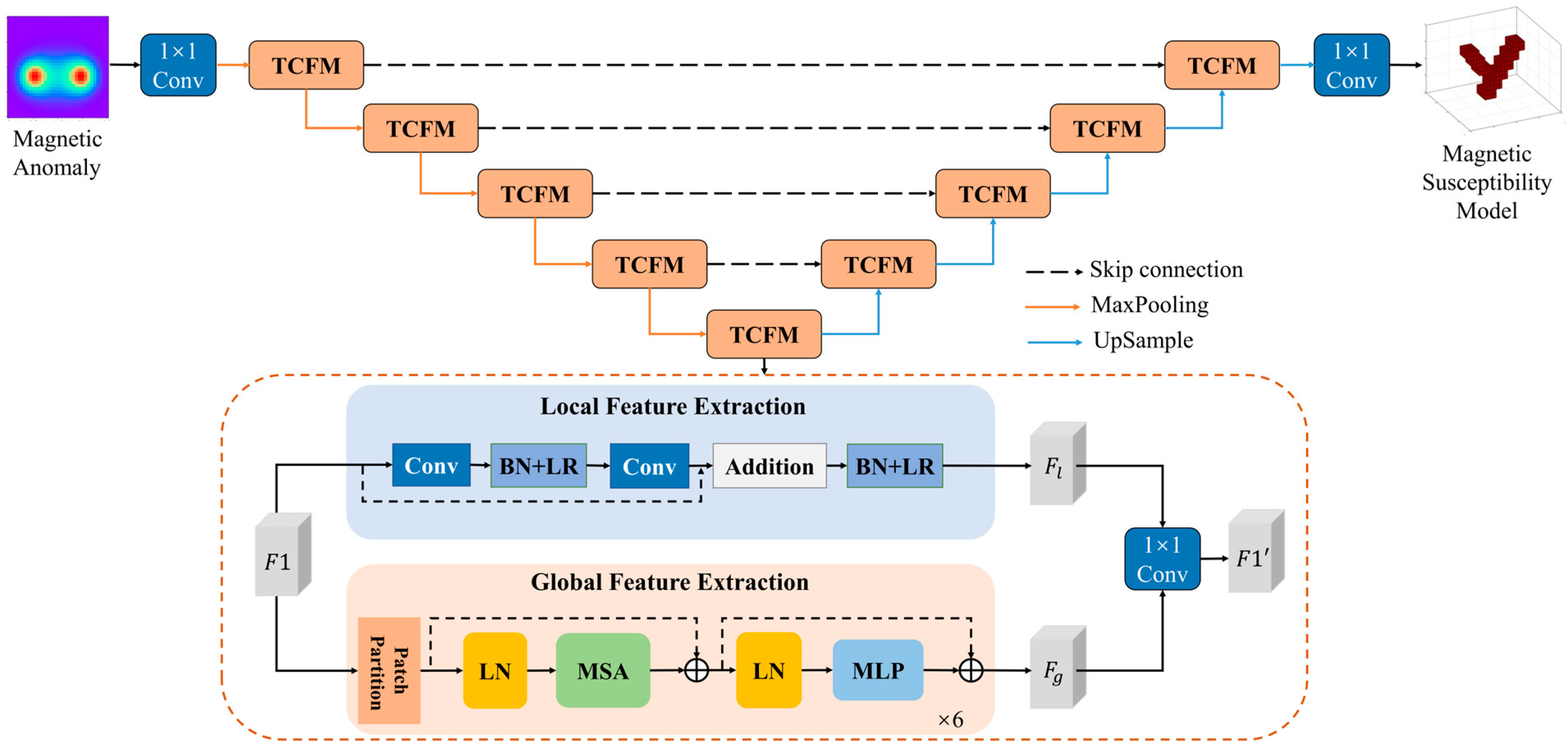
Figure 1. Network Architecture Based on Local-Global Information Co-Modeling.
Applsci 15 12323 g001
Figure 2. (a,b) are models randomly selected from the training set; (c) is the network training loss function.
Applsci 15 12323 g002
Figure 3. Inversion flowchart.
Applsci 15 12323 g003
Figure 4. Synthetic models and forward magnetic anomalies. (a) is Model One; (b) is Model Two; (c) is Model Three; (d) is Model Four; (e) is the forward magnetic anomaly of Model One; (f) is the forward magnetic anomaly of Model Two; (g) is the forward magnetic anomaly of Model Three; (h) is the forward magnetic anomaly of Model Four.
Applsci 15 12323 g004
Figure 5. Model one inversion results. (a) the inversion result using the proposed method in this paper; (b) shows the inversion result using U-Net++; (c) shows the inversion result using ViT; (d), (e), and (f) represent the forward modeling magnetic anomalies for (a), the forward modeling magnetic anomalies for (b), and the forward modeling magnetic anomalies for (c), respectively; (gi) are the residuals of the true magnetic anomaly and (df), respectively.
Applsci 15 12323 g005
Figure 6. Model Two inversion results. (a) the inversion result using the proposed method in this paper; (b) shows the inversion result using U-Net++; (c) shows the inversion result using ViT; (df) are profiles of the three inversion results at X = 1.2 km; (gi) represent the forward modeling magnetic anomalies for (ac), respectively; (jl) are the residuals of the true magnetic anomaly and (gi), respectively.
Applsci 15 12323 g006
Figure 7. Model Three inversion results. (a) the inversion result using the proposed method in this paper; (b) shows the inversion result using U-Net++; (c) shows the inversion result using ViT; (df) are profiles of the three inversion results at X = 2.3 km; (gi) represent the forward modeling magnetic anomalies for (ac), respectively; (jl) are the residuals of the true magnetic anomaly and (gi), respectively.
Applsci 15 12323 g007
Figure 8. Model Four inversion results. (a) the inversion result using the proposed method in this paper; (b) shows the inversion result using U-Net++; (c) shows the inversion result using ViT; (df) are profiles of the three inversion results at X = 2.3 km; (gi) represent the forward modeling magnetic anomalies for (ac), respectively; (jl) are the residuals of the true magnetic anomaly and (gi), respectively.
Applsci 15 12323 g008
Figure 9. (a,d) are magnetic anomalies after adding 6% noise; (b,e) are, respectively, the inversion results of this method and the U-Net inversion results; (c,f) represent the forward modeling magnetic anomalies for (b), and the forward modeling magnetic anomalies for (e), respectively.
Applsci 15 12323 g009
Figure 10. (a) Map of the study area location, (b) Regional geological map (the blue box represents the research area).
Applsci 15 12323 g010
Figure 11. (a) Unmanned Aerial Vehicle (UAV) and Aeromagnetic System; (b) Measured Area Environmental Map; and (c) Study Area Profile Line Map.
Applsci 15 12323 g011
Figure 12. (a) represents the actual magnetic anomaly; (b) represents the inversion result; (c) Residuals between the forward modeling results and the measured magnetic anomalies in (a,d) is the projection of the inversion result onto the XY-plane.
Applsci 15 12323 g012
Figure 13. Slices of the Inversion Results (from left to right: X = 0.5 km, 1.0 km, 1.5 km, 2.0 km, 2.5 km, 3.0 km).
Applsci 15 12323 g013
Table 1. Comparison of computational efficiency.
ModelParameters (Million)Training TimeInference Time
Transformer-CNN20.64.8 h0.35 s
U-Net++10.12.3 h0.25 s
Traditional TikhonovN/AN/A1.8 min
Table 2. Ablation experiment results (Take Model Four as an example).
The Deep Weighting Function Proposed in This PaperMSE + Li & Oldenburg Depth WeightingMSE
Transformer-CNN E m
E d
0.523
1.012
0.609
1.206
0.664
1.215
U-Net++ E m
E d
0.682
1.371
0.774
1.585
0.806
1.684
Disclaimer/Publisher’s Note: The statements, opinions and data contained in all publications are solely those of the individual author(s) and contributor(s) and not of MDPI and/or the editor(s). MDPI and/or the editor(s) disclaim responsibility for any injury to people or property resulting from any ideas, methods, instructions or products referred to in the content.